A Comparative Study on Data Perturbation with Feature Selection

A Comparative Study on Data Perturbation with

Feature Selection

Pengpeng Lin, Jun Zhang, Ingrid St. Omer, Huanjing Wang, and Jie Wang

Abstract—As a major concern in designing various data mining applications, privacy preservation has become a crit-ical component seeking a trade-off between mining utilities and protecting sensitive information. Data perturbation or distortion is a widely used approach for privacy protection. Either by adding noises or matrix decomposition methods, many algorithms were developed based on the simulation of attacker’s behaviors. Most of them are complicated and computationally infeasible on dataset with huge attribute space. In addition, the real-world data tend to be inconsistent, re-dundant and consist of irrelevant part to target information. Executing algorithms on such data is costly and ineffective. Data preprocessing routines attempt to smooth out noise while identifying outliers, and correct inconsistencies in the data. One of the most important data preprocessing techniques is feature selection. In this paper, we intensively studied Singular Value Decomposition (SVD) based data distortion strategy and feature selection techniques, and conducted experiments to explore how feature selection approaches should be used and better serve for privacy preservation purpose. Sparsified Singular Value Decomposition (SSVD) and filter based feature selection are used for data distortion and reducing feature space. We propose a modified version of Exponential Threshold Strategy(ETS) as our threshold function for matrix sparsification. Some metrics are used to measure data distortion level. We also proposed a novel algorithm to compute rank and gave its lower running time bound. The mining utility of distorted data is tested with a well known Classifier, Support Vector Machine (SVM).

Index Terms—SVD; SSVD; SVM; feature selection; pertur-bation

I. INTRODUCTION

P

RIVACY preserving data mining (PPDM) and privacy preserving data publishing (PPDP) are two closely re-lated research directions. The former concentrates on privacy issues when data miners requesting real data for the mining purpose; The latter stresses on an application-free protection of data whenever in need of publishing data for business transactions or research purpose. Both of them disguise dataset in an effort to replace the original dataset for data publications and data mining applications. With the rapid growth of data exchange technology, collaborations with

Manuscript received December 30, 2010; revised January 13, 2011. P.Lin is currently a PHD student in the Department of Computer Sci-ence, University of Kentucky, Lexington, KY, 40506-0046 USA. e-mail: [email protected]. P.Lin would like to thank the Kentucky-West Virginia Alliance for Minority Participation Program (NSF Award #0603091) for supporting his graduate research.

J.Zhang is a Professor in the Department of Computer Science, University of Kentucky, Lexington, KY, 40506-0046 USA. e-mail: [email protected] Ingrid St. Omer is an Assistant Professor in the Department of Electrical and Computer Engineering, University of Kentucky, Lexington, KY, 40506-0046 USA. e-mail: [email protected]

H.Wang is an Assistant Professor in the Department of Mathematics & Computer Science, Western Kentucky University, Bowling Green, KY, 42101-1076 USA. e-mail: [email protected]

J.Wang is an Assistant Professor in the Computer Information System Department, Indiana University Northwest, Gary, Indiana, 46408 USA. e-mail: [email protected]

mining quality and data distortion level respectively. The remainder of the paper is organized as follows. Sect.II looks briefly at the SVD and SSVD processes, feature selec-tion methods, and SVM method. Sect.III discusses various data distortion metrics, their usages and we propose a novel algorithm to compute rank and estimate its lower running time bound. The experiments are carried out and the results are presented and discussed in Sect.IV. We finally sum up this paper and bring our future plans in Sect.V.

II. BACKGROUND ANDRELATEDWORK

A. Singular Value Decomposition

Singular value Decomposition (SVD) is a popular method in data mining and information theory, since it has some very nice mathematical properties.

• Def: Any matrix A ∈ Rm×n can be decomposed uniquely as:

A=U DVT (1)

U is m×m orthonormal matrix, V is n×n orthonormal matrix. D is m×n diagonal matrix whose non-negative entries on its diagonal are called singular values. Let

δ(σ1, σ1, . . . , σk) = diag(D), where k = min(m, n), the singular values are ordered such that σ1 ≥ σ2, . . . ,≥ σk.

And λi ⊆(σ21, σ22, . . . , σ2k) ∀i∈[1, k], where λi represents the egienvalues ofAT_{A. Letx}

ibe the eigenvector belonging toλi. It follows that:

kAxik

2

=xTiATAxi=λixTixi=λikxik

2

(2)

Hence

λi= kAxik

2

kxik

2 (3)

The equation (3) shows that the induced operator two norm of A equals σ1. Since the rank of A equals the number of

singular values, It further implicates that the main charac-teristics of A can be captured by lower rank items. On the other hand, the singular values around the bottom of the diagonal of D are relatively small and insignificant. If we introduce perturbations on those insignificant singular values i.e., making them zero, we can represent A in a perturbed formA¯. Furthermore, letE=A−A¯, then, the removed part

E can be considered as noise inA[7]. Thus,A¯can be seen as both a distorted copy ofAand a faithful representation of the original data [4].

B. Sparsified SVD

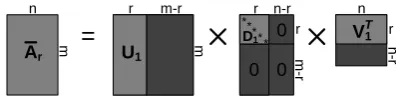
In order to sparsify a matrix A, we can set a threshold and the entry values of A less than the threshold are set to zero. The rank of original matrix A is reduced when we apply this strategy to the matrix D. It can be seen from Figure 1 that a distorted matrix A¯rcan be composed with dimension reduced matrices by doing simple block matrix operations:

¯

Ar=U1D1V1T (4)

where U1 is an m×r matrix, D1 is a r×r matrix, and an V1T isr×nmatrix.

To increase distortion level, we also set small entries in U1

andV1T less than predefined threshold zero. Such operation

n

m

Ar

=

U1

r m-r

m

** * * *

D1 0

0 0

V1 n

r r n-r

n

-r

m

-r

[image:2.595.327.530.52.104.2]

r T

Fig. 1. Singular Value Decomposition

is referred to as dropping operation in [2]. Therefore, the SSVD can be seen as a process further perturbing the matrix

A:

A= ¯Ar+E1+E2 (5)

After dropping operations on the small entries inU1andV1T,

the significant values are still kept, thus the mining utility of

Ais well preserved and distorted twice at the same time. Threesparsificationstrategies were proposed in [2], where the Exponential Threshold Strategy (ETS) showed the best empirical results. In our work, we propose a modified ETS threshold function:METS. METS, as in (6), defines a smooth threshold function using an exponential function in which the threshold value is customized for each column of the matrix.

Tj =

m

m X

i=1

|aij|ej·r

−2

(6)

The original ETS threshold formula is modified in METS by having parameter α redefined. Rather than setting different value for α every time, we substitute it with a fraction number r−1_{, whose magnitude is determined by r, which}

is the number of the singular values kept. The computed threshold value for each column is adjustable with scaling factor. Note that different from ETS, the absolute value of

aij is computed in METS. This is because that during SVD decomposition, some of the entries in decomposed matrices U and V might become negative. As a result, the threshold calculated based on the original ETS formula may be large for low rank items and small for high rank items. Calculating threshold value with absolute entry value ensures that larger threshold values are computed for entry value with higher column index. Therefore, the most important entries are kept, whereas more trivial entries will be dropped to zero.

C. Feature Selection

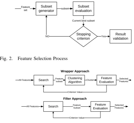
Feature selection research has found applications in many fields where large volumes of data present challenges to effective data analysis and processing. As data evolve to be ubiquitous and abundant, new challenges arise everyday and expectations of feature selection are also elevated. Feature selection algorithms have two main components: feature searchandfeature subset evaluation.

Feature search strategies have been widely used for

searching feature space. An exhaustive search would cer-tainly find the optimal solution; however, for a dataset of

Subset generator

Subset evaluation

Result validation Stopping

criterion

Feature

set subset

Current best subset

[image:3.595.47.271.54.260.2]

Yes NO

Fig. 2. Feature Selection Process

Clustering Algorithm

Feature Evaluation Search

All Features Feature_subset Clusters Selected_Features

Criterion Value

Search Feature Evaluation Feature

Subset

All Features Selected

Features

Criterion Value

Wrapper Approach

Filter Approach

Fig. 3. Filter and Wrapper Approaches

a time. Whitney [6] introduced sequential forward selection, which starts with empty set and sequentially adds one feature at a time. Random search methods such as genetic algorithms add some randomness in the search procedure to escape from a local optimum. Individual search methods evaluate each feature individually and select features that either satisfy the condition or are top-ranked. In our work, a sequential search

Best First Search (BFS) is used.

Feature subset evaluation process as in Figure 2 is used to

identify irrelevant and redundant features. In classification, the feature evaluation criterions are naturally related to the labeled classes, thus filter based methods are often used. In clustering where class labels may be unavailable, either filter or wrapper approaches are used. As shown in Figure 3, the wrapper approach wraps the feature search by learning algorithms whereas filter approach utilizes the intrinsic prop-erty of the data alone to select feature subspace. Intuitively, wrapper approach may result in a better performance. How-ever, wrapper methods are more expensive since they run the learning algorithm for each candidate feature subset. In our experiments, we use filter method as we use SVM classifier for data utility metric.

D. Support Vector Machine

In this paper, Support Vector Machine (SVM) is chosen as the data utility measure to assess how much a dataset keeps the analytical values of data mining techniques after the data distortion. SVM is a method for classification. It uses a nonlinear mapping to transform the original training data that are linearly inseparable into a higher dimension. It then searches for the linear optimal separating hyperplane.

A hyperplane that separates data from different classes can

always be found by mapping data into a sufficiently high dimension. The basic SVM process is shown in Figure 4. Essentially two hyperplanesH1, H2 with maximummargin

are defined for every class pairs. Any training tuples that fall on H1 or H2 are calledsupport vectors. Tuples that falls on or above H1 belong to class A, and tuples that falls on or

B

B

B B A

B

A

B A

A

Largest _margin

Small margin

Class A Class B Support vector H1

[image:3.595.329.523.56.185.2]

H2

Fig. 4. Support Vector Machine

below H2 belong to class B. The SVM finds thehyperplane

usingsupport vectors and maximummargins.

III. DATADISTORTIONMEASUREMENTS

Data distortion metrics are used to measure the degree of data distortion. In this paper, we implemented the metrics that were introduced in the literatures [3, 4]. These metrics are designed based on the original data Aand its perturbed counterpartA¯.

A. Value Difference(VD)

After a data distortion, the distance between original data and perturbed data is measured by their relative changes as shown in (7). Frobenius norm is used to map matrix A ∈

Rm×n toR.

V D=

A−A¯

_F

kAk_F (7)

B. Rank Difference(RD)

To measure data position changes, the values in each column are ranked in an ascending order. The ranks change between original data and perturbed data after distortion.

Rank Position (RP) and Rank Maintenance (RM) [3,4] are

used here. RP is used to denote the average change of rank for all the data values. RM represents the percentage of elements that keep their ranks of magnitude in each column after the distortion [3].

One may infer the content of one feature from its relative value difference compared with the other attributes. Thus it is desirable that the order of the average value of each attribute varies after the data distortion [4]. The rank of a feature is assigned according to its average value.Change of

Rank of Features(CP) andMaintenance of Rank of Features

(CK) [3,4] are used in our work to indicate the changes of rank of the average value of the features and assess the percentage of the features that keep their ranks after the distortion. Interested readers might refer to [3,4] for a detailed description.

C. Compute Ranks(CR)

Algorithm 1 Compute Ranks (CRK)

Require: m×nDataSet S,A[m][n][3]

Ensure: Numerical Data Type

1: fori= 1to ndo

2: forj= 1 tom do

3: A(j, i)[1]←S(j, i)

4: A(j, i)[2]←j

5: end for

6: end for

7: Sort Col(A) by A(, n)[1]

8: fori= 1to ndo

9: forj= 1 tom do

10: A(j, i,3)←j

11: end for

12: end for

13: Sort Col(A) by A(, n)[2]

14: return A(,)[3]

In theAlgorithm 1,Ais a multidimensional array, and each cell can hold up to 3 values. We use notationA(m, n)[x]to represent each value in A. For example, A(i, j)[k] denotes for the kth _{value of the entry in i}th _{row and j}th _column, where k∈[1,3]. Similarly, S(i, j) denotes the data entry in

ith _{row and j}th _{column ofS. If m and n are not specified,} the whole row or the whole column is being considered. For example, A(, j)[k] denotes for thekth value in jth column andA(, n)[k] denotes for thekthvalue of each entry in all the columns.

In the steps 1-6 of the Algorithm, the 1st _and2nd _values of entry in A are assigned with the data values in S and their corresponding row index respectively. We then sort each column of A in ascending order by the first value in each entry in step 7. In the steps 8-12 we assign the3rdvalue of each entry in A with the current corresponding row index. Finally, we sort each column ofAin ascending order by the second value in corresponding entry in step13. Step13 is to rearrange A back to the original form. The 3rd _{values in a} newly arranged order after step13 form a nice rank table.

We also define that if two elements in the data table have the same value, the element with the lower row index to have the higher rank. Assuming that the data set is ann×n

square matrix, since comparison based sorting algorithms have lower bound o(nlog(n)) and CRK sorts the data twice for each column, the estimated time is o(2n2_{log(n)). Since}

it is not growing exponentially, for a large scale data set, this is an acceptable computation cost.

IV. EXPERIMENTS ANDRESULTS

We conduct experiments to test the performance of the SVM on distorted data produced by feature selection and data perturbation procedure in different sequence. The results are compared with outcomes produced by performing SVM on original data without any distortion. The sequence that generates closer result to the result produced from original data without perturbation is considered preserving better mining utility. The data distortion level and degree of feature selection are also compared and contrasted with metrics discussed in Sect.III.

A. Setup and Dataset

We implemented dropping strategy METS for matrix spar-sification, all five data distortion measures described in [3,4] and simulated decomposition and composition processes of SVD method. We download “Wisconsin Breast Cancer (Di-agnostic)” data set and Connectionist Bench (Sonar, Mines vs. Rocks) data set from [8,9]. The Wisconsin Breast Cancer data set has 32 features, such as diagnosis, texture, smooth-ness, concavity, concave points, fractal dimension, etc. These features are computed from a digitized image of a fine needle aspirate (FNA) of a breast mass. They describe characteristics of the cell nuclei present in the image. The target feature is Diagnosis: “B” = benign, “M” = malignant. The dimension of the data matrix is569×32. Connectionist Bench data set has 60 features and 208 instances. This data set contains patterns obtained by bouncing sonar signals off a metal cylinder or rocks at various angles and under different conditions. Each pattern is a set of 60 numbers in the range from 0.0 to 1.0, which represents the energy within a particular frequency band integrated over a certain period of time. For the target feature, the label associated with each record is letter “R” if the object is rock and “M” if it is a metal cylinder.

Correlation-based feature evaluator is used to assess the worthiness of a feature subset by considering the individual predictive ability of each feature along with the degree of re-dundancy between them. We choose Best First Search (BFS) to search the feature space by greedy hill climbing either augmented with a forward tracking facility or decremented with a backward searching facility.

B. Experiment 1

In experiment 1, we perform feature selection (Fs) on original data (Org) without any data distortion. We then use SVM to generate the correct predict rate. Ten folds cross validation is set to split the data in 10 approximately equal partsD1, . . . , D10. Training setDti is obtained by removing part ofDi from D.

TABLE I SVM RESULTS

DataSet: WBC Sonar

exp# F Size SVM Rate F Size SVM Rate

Org 32 97.89% 60 75.96%

F s 12 96.66% 19 77.40%

Ep2 12 92.26% 19 76.44%

Ep3 7 90.86% 13 75.00%

correct predict rate, which indicates that both data sets consist of large proportion of unwanted information that has very little perturbation values. Applying data distortion procedure on selected feature space would result in better performance.

C. Experiment 2

In experiment 2, we carried out the experiment in the sequence that performing feature selection before data distor-tion. We select feature subspace on original data. A new data set is then formed with selected feature subspace. We only perform distortion on selected feature space as it has high perturbation values and the discarded features are considered irrelevant or trivially related to target feature. We treat the newly form data set as a matrix and perform SVD on it. We then use the sparsification strategies discussed in Sect II on decomposed matrices U and V. For each singular values

σi on the diagonal of decomposed matrix D, we define the sparsification rule as follows:

σi=

σi ifσi>1

0 otherwise (8)

Only the singular values greater than one are kept. For the decomposed matrices U and V, we use MEST to compute threshold value ζ for each column. The scaling parameter

of METS is set to be 0.6. The entry values in U and V less than ζ are set to zero, or remain untouched otherwise. To be consistent, both data sets are perturbed using the same settings. After sparsification, a perturbed data matrix is recomposed by multiplications of the sparsified matrices

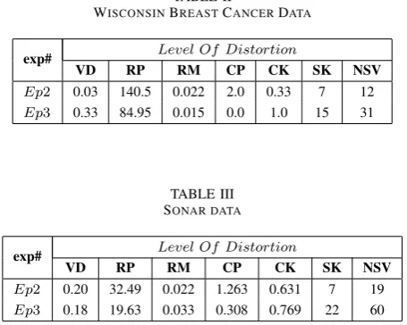
U,D andVT. We then assess its distortion levels according to the distortion metrics discussed in Sect. III. The data distortion level results are shown in Table II and Table III below, where NSV stands for number of singular values, and SK stands for number of singular values kept after sparsification.

TABLE II

WISCONSINBREASTCANCERDATA

exp# Level Of Distortion

VD RP RM CP CK SK NSV

Ep2 0.03 140.5 0.022 2.0 0.33 7 12

Ep3 0.33 84.95 0.015 0.0 1.0 15 31

TABLE III SONAR DATA

exp# Level Of Distortion

VD RP RM CP CK SK NSV

Ep2 0.20 32.49 0.022 1.263 0.631 7 19

Ep3 0.18 19.63 0.033 0.308 0.769 22 60

We can see from results that VD and RP values for both data sets appear to be small due to the small data entry values. The RM values and CK values, on the other hand, explicitly indicates that both data sets are well perturbed. It shows that only 2.2% data ranks are kept unchanged for both WBC data, and Sonar data. 67% ranks of the average feature value are changed for WBC and 36.9% for Sonar data

97.89%

96.66%

92.26% 90.88%

75.96% 77.40% _76.44% 75.00%

65.00% 70.00% 75.00% 80.00% 85.00% 90.00% 95.00% 100.00%

[image:5.595.56.284.508.690.2]

Org Fs Ep2 Ep3 SVM(WBC) SVM(Sonar)

Fig. 5. SVM Rate Comparisons

sets. From the data utility results shown in Table I, there is no significant changes in overall correct predict rate. The interesting thing is that, after data distortion, the predictive power of SVM is still better than the correct predict rate for original data (Org) by 0.48 percent. This demonstrates SVD’s ability to rule out trivial values and noises. After removing those insignificant entry values during sparsification process, the data are ”purified” and thus result in better mining performance.

D. Experiment 3

In comparison with experiment 2, we carried out the experiment 3 in a reversed sequence. We instead, distort original data using SVD first, and then select features on perturbed data. Again, we use SVM to generate correct predict rate. The parameter settings and configuration for data distortion and SVM are the same as in Experiment 1 and Experiment 2 for consistency purpose.

The Figure 5 shows the SVM results for both data sets in different experiments. As we can see, There is no significant differences in SVM predict rates for all experiments. As shown in both Table I and Figure 5, the results for SVM rate in Experiment 3 followed a similar trend to Experiment 2, although the data distortion degree is better. Particularly for the WBC data as shown in Table II, the ranks of the average value for each feature stayed the same in Experiment 3, but changed greatly in Experiment 2 by 67%. From the feature selection’s perspective, Experiment 3 has better results for both data sets. The sizes of selected feature space for both data sets have evident drops with only insignificant impacts on SVM results, which is a further empirical evidence of SVD’s ability to filter out noises.

E. Summary

By comparing the empirical results, some important and interesting facts can be drawn from our observations.

• The results in our experiments indicate that, for

classi-fication purpose, data owner publishing perturbed data before feature selection results in no significant differ-ence in correct predict rate than the other way around.

• Data distortion process should be done on selected fea-ture space. The discarded feafea-tures by feafea-ture selection procedure have very little perturbation values.

to eliminate garbage information and improve mining qualities.

• For Feature Selection, performing feature selection

pro-cess after sparsification propro-cess by SSVD would result in better outcomes, i.e. more irrelevant features can be identified.

Based on the facts listed above, we conclude that perform-ing feature selection before data perturbation is a better ap-proach than the other way around for classification purpose, since there is no major distinguishable contrasts in predict outcomes and discarded features have little perturbation values. On the other hand, the perturbed data published by data owner also have little effects on correct predict rate, but could result in significantly better feature selection results. Empirical tests are required for choosing the rank of SVD and setting proper threshold parameters. How many singular values to keep or how large a threshold should be set is different from applications to applications and, of course, is dependent on the nature of the data to be distorted.

V. CONCLUSIONANDFUTUREPLANS

In this paper, we studied Singular Value Decomposition (SVD), Sparsified Singular value Decomposition (SSVD), Support Vector Machine (SVM), and various data distortion metrics. We proposed a new threshold function METS which is based on ETS and takes negative entry values into consid-eration. We also proposed a novel algorithm to compute rank and give a theoretical lower run time bound. The empirical results in our work indicate that feature selection methods should be performed before perturbing data for classification. In the future, we would like to try more real world data sets as well as synthetic data sets, and carry out experiments with more data distortion methods on other data mining applications such as association rules, clustering etc.

REFERENCES

[1] Z. Yang, S. Zhong, R.N. Wright,“Privacy-preserving classification of customer data without loss of accuracy”In Proceedings of the 5th SIAM International Conference on Data Mining, Newport Beach, CA, April 21-23, 2005

[2] J. Gao, J. Zhang.“Sparsification strategies in latent semantic indexing”

In Proceedings of the 2003 Text Mining Workshop, M.W. Berry and W.M. Pottenger, (ed.), pp. 93-103, San Francisco, CA, May 3, 2003 [3] S. Xu, J. Zhang, D. Han,J. Wang,“Data distortion for privacy

protec-tion in a terrorist analysis system”In Proceedings of the 2005 IEEE International Conference on Intelligence and Security Informatics, pp. 459-464, Atlanta, GA, May 2005.

[4] J. Wang, W. Zhong, S. Xu, J. Zhang,“Selective Data Distortion via Structural Partition and SSVD for Privacy Preservation”In Proceedings of the 2006 International Conference on Information & Knowledge Engineering, pp:114-120, CSREA Press, Las Vegas

[5] T. Marill, D.M. Green.“On the effectiveness of receptors in recognition systems”. IEEE Transations on Information Theory, 9:11-17, 1963. [6] A.W. Whitney.“A direct method of nonparametric measurement

selec-tion”. IEEE Transactions on Computers, 20:1100-1103, 1971. [7] Berry MW, Drmac Z, Jessup ER“Matrix,Vector space, and information

retrieval”. SIAM Rev 41:355-361

[8] William H. Wolberg and O.L. Mangasarian“Multisurface method of pattern separation for medical diagnosis applied to breast cytology”. Proceedings of the National Academy of Sciences, U.S.A., Volume 87, December 1990, pp 9193-9196.