Generic binarization for parsing and translation
Matthias B¨uchse Technische Universit¨at Dresden
Alexander Koller University of Potsdam [email protected]
Heiko Vogler
Technische Universit¨at Dresden [email protected]
Abstract
Binarization of grammars is crucial for im-proving the complexity and performance of parsing and translation. We present a versatile binarization algorithm that can be tailored to a number of grammar for-malisms by simply varying a formal pa-rameter. We apply our algorithm to bi-narizing tree-to-string transducers used in syntax-based machine translation.
1 Introduction
Binarization amounts to transforming a given grammar into an equivalent grammar of rank 2, i.e., with at most two nonterminals on any right-hand side. The ability to binarize grammars is crucial for efficient parsing, because for many grammar formalisms the parsing complexity de-pends exponentially on the rank of the gram-mar. It is also critically important for tractable statistical machine translation (SMT). Syntax-based SMT systems (Chiang, 2007; Graehl et al., 2008) typically use some type ofsynchronous grammar describing a binary translation rela-tion between strings and/or trees, such as syn-chronous context-free grammars (SCFGs) (Lewis and Stearns, 1966; Chiang, 2007), synchronous tree-substitution grammars (Eisner, 2003), syn-chronous tree-adjoining grammars (Nesson et al., 2006; DeNeefe and Knight, 2009), and tree-to-string transducers (Yamada and Knight, 2001; Graehl et al., 2008). These grammars typically have a large number of rules, many of which have rank greater than two.
The classical approach to binarization, as known from the Chomsky normal form transfor-mation for context-free grammars (CFGs), pro-ceeds rule by rule. It replaces each rule of rank greater than 2 by an equivalent collection of rules of rank 2. All CFGs can be binarized in this
way, which is why their recognition problem is cubic. In the case of linear context-free rewriting systems (LCFRSs, (Weir, 1988)) the rule-by-rule technique also applies to every grammar, as long as an increased fanout it permitted (Rambow and Satta, 1999).
There are also grammar formalisms for which the rule-by-rule technique is not complete. In the case of SCFGs, not every grammar has an equiva-lent representation of rank 2 in the first place (Aho and Ullman, 1969). Even when such a represen-tation exists, it is not always possible to compute it rule by rule. Nevertheless, the rule-by-rule bi-narization algorithm of Huang et al. (2009) is very useful in practice.
In this paper, we offer a generic approach for transferring the rule-by-rule binarization tech-nique to new grammar formalisms. At the core of our approach is a binarization algorithm that can be adapted to a new formalism by changing a pa-rameter at runtime. Thus it only needs to be im-plemented once, and can then be reused for a va-riety of formalisms. More specifically, our algo-rithm requires the user to (i) encode the grammar formalism as a subclass ofinterpreted regular tree grammars(IRTGs, (Koller and Kuhlmann, 2011)) and (ii) supply a collection ofb-rules, which rep-resent equivalence of grammars syntactically. Our algorithm then replaces, in a given grammar, each rule of rank greater than 2 by an equivalent collec-tion of rules of rank 2, if such a colleccollec-tion is li-censed by the b-rules. We define completeness of b-rules in a way that ensures that if any equivalent collection of rules of rank 2 exists, the algorithm finds one. As a consequence, the algorithm bina-rizes every grammar that can be binarized rule by rule. Step (i) is possible for all the grammar for-malisms mentioned above. We show Step (ii) for SCFGs and tree-to-string transducers.
We will use SCFGs as our running example throughout the paper. We will also apply the
rithm to tree-to-string transducers (Graehl et al., 2008; Galley et al., 2004), which describe rela-tions between strings in one language and parse trees of another, which means that existing meth-ods for binarizing SCFGs and LCFRSs cannot be directly applied to these systems. To our knowl-edge, our binarization algorithm is the first to bi-narize such transducers. We illustrate the effec-tiveness of our system by binarizing a large tree-to-string transducer for English-German SMT.
Plan of the paper. We start by defining IRTGs in Section 2. In Section 3, we define the gen-eral outline of our approach to rule-by-rule bina-rization for IRTGs, and then extend this to an ef-ficient binarization algorithm based on b-rules in Section 4. In Section 5 we show how to use the algorithm to perform rule-by-rule binarization of SCFGs and tree-to-string transducers, and relate the results to existing work.
2 Interpreted regular tree grammars Grammar formalisms employed in parsing and SMT, such as those mentioned in the introduc-tion, differ in the the derived objects—e.g., strings, trees, and graphs—and the operations involved in the derivation—e.g., concatenation, substitution, and adjoining. Interpreted regular tree grammars (IRTGs) permit a uniform treatment of many of these formalisms. To this end, IRTGs combine two ideas, which we explain here.
Algebras IRTGs represent the objects and op-erations symbolically using terms; the object in question is obtained by interpreting each symbol in the term as a function. As an example, Table 1 shows terms for a string and a tree, together with the denoted object. In the string case, we describe complex strings as concatenation (con2) of
ele-mentary symbols (e.g., a, b); in the tree case, we alternate the construction of a sequence of trees (con2) with the construction of a single tree by
placing a symbol (e.g.,α, β, σ) on top of a (pos-sibly empty) sequence of trees. Whenever a term contains variables, it does not denote an object, but rather a function. In the parlance of universal-algebra theory, we are employing initial-algebra semantics(Goguen et al., 1977).
Analphabetis a nonempty finite set. Through-out this paper, let X = {x1, x2, . . .} be a set,
whose elements we callvariables. We let Xk
de-note the set{x1, . . . , xk}for everyk ≥ 0. LetΣ
be an alphabet andV ⊆ X. We writeTΣ(V)for
the set of all terms overΣwith variablesV, i.e., the smallest setT such that (i)V ⊆T and (ii) for every σ ∈ Σ, k ≥ 0, and t1, . . . , tk ∈ T, we
have σ(t1, . . . , tk) ∈ T. Alternatively, we view
TΣ(V) as the set of all (rooted, labeled, ordered,
unranked) trees over Σ and V, and draw them as usual. By TΣ we abbreviate TΣ(∅). The set
CΣ(V) of contexts overΣandV is the set of all
trees over Σ andV in which each variable in V occurs exactly once.
Asignatureis an alphabetΣwhere each symbol is equipped with an arity. We write Σ|k for the
subset of allk-ary symbols ofΣ, andσ|kto denote
σ ∈ Σ|k. We denote the signature by Σas well.
A signature isbinaryif the arities do not exceed2. Whenever we useTΣ(V) with a signature Σ, we
assume that the trees are ranked, i.e., each node labeled byσ∈Σ|khas exactlykchildren.
Let∆be a signature. A∆-algebraAconsists of a nonempty set A called the domain and, for each symbolf ∈ ∆with rankk, a total function fA: Ak → A, the operation associated with f. We can evaluate any term tin T∆(Xk) inA, to
obtain ak-ary operationtA over the domain. In particular, terms inT∆evaluate to elements ofA.
For instance, in the string algebra shown in Ta-ble 1, the termcon2(a, b)evaluates toab, and the
term con2(con2(x
2, a), x1) evaluates to a binary
operationf such that, e.g.,f(b, c) =cab.
Bimorphisms IRTGs separate the finite control (state behavior) of a derivation from its derived object (in its term representation; generational be-havior); the former is captured by a regular tree language, while the latter is obtained by applying a tree homomorphism. This idea goes back to the tree bimorphismsof Arnold and Dauchet (1976).
LetΣbe a signature. Aregular tree grammar (RTG) G over Σ is a triple (Q, q0, R) where Q
is a finite set (of states), q0 ∈ Q, and R is a
fi-nite set of rules of the formq → α(q1, . . . , qk),
where q ∈ Q, α ∈ Σ|k and q, q1, . . . , qk ∈ Q.
We call α the terminal symbol and k the rank of the rule. Rules of rank greater than two are called suprabinary. For every q ∈ Q we de-fine thelanguageLq(G)derived fromq as the set
{α(t1, . . . , tk) | q → α(q1, . . . , qk) ∈ R, tj ∈
Lqj(G)}. Ifq = q
0, we drop the superscript and
strings overΓ trees overΓ
example term and denoted object
con2
a b 7→ab
σ
con2
α
con0
β
con0
7→
σ
α β
domain Γ∗ TΓ∗(set of sequences of trees) signature∆ {a|0 |a∈Γ} ∪ {γ|1|γ∈Γ} ∪
{conk|
k|0≤k≤K, k6= 1} {conk|k|0≤k≤K, k6= 1}
operations a: ()7→a γ:x1 7→γ(x1)
[image:3.595.82.516.62.240.2]conk: (x1, . . . , xk)7→x1· · ·xk conk: (x1, . . . , xk)7→x1· · ·xk
Table 1: Algebras for strings and trees, given an alphabetΓand a maximum arityK ∈N.
or none. This does not increase the generative ca-pacity (Brainerd, 1969).
A(linear, nondeleting) tree homomorphismis a mapping h: TΣ(X) → T∆(X) that satisfies the
following condition: there is a mapping g: Σ → T∆(X) such that (i) g(σ) ∈ C∆(Xk) for every
σ ∈ Σ|k, (ii)h(σ(t1, . . . , tk))is the tree obtained
from g(σ) by replacing the occurrence of xj by
h(tj), and (iii) h(xj) = xj. This extends the
usual definition of linear and nondeleting homo-morphisms (G´ecseg and Steinby, 1997) to trees with variables. We abuse notation and writeh(σ) forg(σ)for everyσ ∈Σ.
Let n ≥ 1 and∆1, . . . ,∆n be signatures. A
(generalized) bimorphism over(∆1, . . . ,∆n)is a
tuple B = (G, h1, . . . , hn) where G is an RTG
over some signature Σ and hi is a tree
homo-morphism from TΣ(X) into T∆i(X). The
lan-guage L(B) induced by B is the tree relation
{(h1(t), . . . , hn(t))|t∈L(G)}.
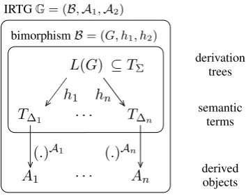
An IRTG is a bimorphism whose derived trees are viewed as terms over algebras; see Fig. 1. Formally, an IRTG G over (∆1, . . . ,∆n) is a
tuple (B,A1, . . . ,An) such that B is a
bimor-phism over(∆1, . . . ,∆n)andAiis a∆i-algebra.
The languageL(G) induced byG is the relation
{(tA1
1 , . . . , tAnn) | (t1, . . . , tn) ∈ L(B)}. We call
the trees in L(G) derivation treesand the terms inL(B)semantic terms. We say that two IRTGs
GandG0areequivalentifL(G) =L(G0). IRTGs
were first defined in (Koller and Kuhlmann, 2011). For example, Fig. 2 is an IRTG that encodes a synchronous context-free grammar (SCFG). It contains a bimorphism B = (G, h1, h2)
consist-ing of an RTG G with four rules and
homomor-L(G)
T∆1 · · · T∆n
A1 · · · An
h1 hn
(.)A1 (.)An ⊆TΣ
bimorphismB= (G, h1, h2) IRTGG= (B,A1,A2)
derivation trees
semantic terms
[image:3.595.325.502.279.420.2]derived objects
Figure 1: IRTG, bimorphism overview.
A→α(B, C, D)
B→α1, C→α2, D→α3
con3
x1 x2 x3
h1 ←−[α h2
7−→ con
4
x3 a x1 x2
b h1
←−[α17−→h2 b
c h1
←−[α27−→h2 c
d h1
←−[α37−→h2 d
Figure 2: An IRTG encoding an SCFG.
phisms h1 andh2 which map derivation trees to
trees over the signature of the string algebra in Ta-ble 1. By evaluating these trees in the algebra, the symbolscon3andcon4are interpreted as
al-con3
b c d
h1 ←−[
α α1 α2 α3
h2
7−→ con
4
d a b c
Figure 3: Derivation tree and semantic terms.
A→α0(A0, D)
A0→α00(B, C)
con2
x1 x2
h0
1 ←−[α0 h02
7−→
con2
con2
x2 a
x1
con2
x1 x2
h0
1 ←−[α00 h02
7−→ con
2
x1 x2
Figure 4: Binary rules corresponding to theα-rule in Fig. 2.
gebras yield tree-adjoining languages (Koller and Kuhlmann, 2012), and algebras over other do-mains can yield languages of trees, graphs, or other objects. Furthermore, IRTGs withn= 1 de-scribe languages that are subsets of the algebra’s domain, n = 2 yields synchronous languages or tree transductions, and so on.
3 IRTG binarization
We will now show how to apply the rule-by-rule binarization technique to IRTGs. We start in this section by defining the binarization of a rule in an IRTG, and characterizing it in terms of binariza-tion termsandvariable trees. We derive the actual binarization algorithm from this in Section 4.
For the remainder of this paper, let G = (B,A1, . . . ,An) be an IRTG over (∆1, . . . ,∆n)
withB= (G, h1, . . . , hn).
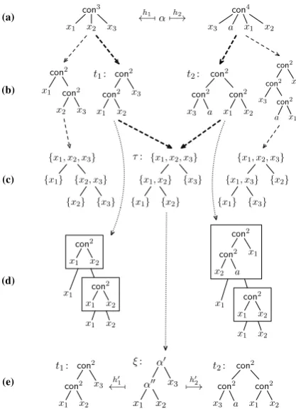
3.1 An introductory example
We start with an example to give an intuition of our approach. Consider the first rule in Fig. 2, which has rank three. This rule derives (in one step) the fragmentα(x1, x2, x3)of the derivation
tree in Fig. 3, which is mapped to the semantic termsh1(α)andh2(α)shown in Fig. 2. Now
con-sider the rules in Fig. 4. These rules can be used to derive (in two steps) the derivation tree fragmentξ in Fig. 5e. Note that the termsh01(ξ) and h1(α)
areequivalent in that they denote the same func-tion over the string algebra, and so are the terms h02(ξ) and h2(α). Thus, replacing the α-rule by
the rules in Fig. 4 does not change the language of the IRTG. However, since the new rules are binary,
(a) con3
x1 x2 x3
con4
x3 a x1 x2
(b)
con2
x1 con2
x2 x3 con2
con2
x1 x2 x3
t1: con2
con2
x3 a con2
x1 x2
t2:
con2
con2
x3 con2
a x1
x2
(c)
(d)
con2
x1 x2
x1 con 2
x1 x2
x1 x2
con2
con2
x2 a x1
x1 con 2
x1 x2
x1 x2
(e)
h1 ←−[α h2
7−→
{x1, x2, x3}
{x1} {x2, x3}
{x2} {x3}
{x1, x2, x3}
{x1, x2}
{x1} {x2} {x3}
τ: {x1, x2, x3}
{x1, x3}
{x1} {x3} {x2}
con2
con2
x1 x2 x3
t1:
h′ 1 ←−[
α′
α′′
x1 x2
x3 ξ: h′ 2 7−→ con2 con2
x3 a con2
x1 x2
[image:4.595.310.519.61.351.2]t2:
Figure 5: Outline of the binarization algorithm.
parsing and translation will be cheaper.
Now we want to construct the binary rules sys-tematically. In the example, we proceed as fol-lows (cf. Fig. 5). For each of the termsh1(α)and
h2(α)(Fig. 5a), we consider all terms that satisfy
two properties (Fig. 5b): (i) they are equivalent toh1(α)andh2(α), respectively, and (ii) at each
node at most two subtrees contain variables. As Fig. 5 suggests, there may be many different terms of this kind. For each of these terms, we ana-lyze the bracketing of variables, obtaining what we call avariable tree(Fig. 5c). Now we pick terms t1 andt2 corresponding toh1(α) andh2(α),
re-spectively, such that (iii) they have the same vari-able tree, sayτ. We construct a treeξfromτ by a simple relabeling, and we read off the tree homo-morphisms h01 andh02 from a decomposition we perform ont1andt2, respectively; see Fig. 5,
dot-ted arrows, and compare the boxes in Fig. 5d with the homomorphisms in Fig. 4. Now the rules in Fig. 4 are easily extracted fromξ.
These rules are equivalent to r because of (i); they are binary becauseξis binary, which in turn holds because of (ii); finally, the decompositions oft1 andt2are compatible withξbecause of (iii).
We call termst1 andt2 binarization termsif they
con-struct binary rules equivalent tor from any given sequence of binarization termst1, t2, and that
bi-narization terms exist whenever equivalent binary rules exist. The majority of this paper revolves around the question of finding binarization terms.
Rule-by-rule binarization of IRTGs follows the intuition laid out in this example closely: it means processing each suprabinary rule, attempting to replace it with an equivalent collection of binary rules.
3.2 Binarization terms
We will now make this intuition precise. To this end, we assume thatr = q → α(q1, . . . , qk)is a
suprabinary rule ofG. As we have seen, binariz-ingrboils down to constructing:
• a treeξover some binary signatureΣ0and
• tree homomorphisms h01, . . . , h0n of type h0i:TΣ0(X)→T∆i(X),
such thath0i(ξ)andhi(α)are equivalent, i.e., they
denote the same function overAi. We call such a
tuple(ξ, h01, . . . , h0n) a binarizationof the ruler. Note that a binarization ofr need not exist. The problem of rule-by-rule binarization consists in computing a binarization of each suprabinary rule of a grammar. If such a binarization does not exist, the problem does not have a solution.
In order to define variable trees, we assume a mapping seqthat maps each finite set U of pair-wise disjoint variable sets to a sequence over U which contains each element exactly once. Let t ∈ C∆(Xk). The variable set oft is the set of
all variables that occur int. Theset S(t)of sub-tree variablesoftconsists of the nonempty vari-able sets of all subtrees of t. We represent S(t) as a treev(t), which we callvariable tree as fol-lows. Any two elements ofS(t)are either compa-rable (with respect to the subset relation) or dis-joint. We extend this ordering to a tree struc-ture by ordering disjoint elements viaseq. We let
v(L) ={v(t)|t∈L}for everyL⊆C∆(Xk).
In the example of Fig. 5,t1andt2have the same
set of subtree variables; it is {{x1},{x2},{x3}, {x1, x2},{x1, x2, x3}}. If we assume thatseq
or-ders sets of variables according to the least vari-able index, we arrive at the varivari-able tree in the cen-ter of Fig. 5.
Now let t1 ∈ T∆1(Xk), . . . , tn ∈ T∆n(Xk).
We call the tuplet1, . . . , tnbinarization termsof
rif the following properties hold: (i)hi(α)andti
are equivalent; (ii) at each node the treeticontains
at most two subtrees with variables; and (iii) the termst1, . . . , tnhave the same variable tree.
Assume for now that we have found binariza-tion termst1, . . . , tn. We show how to construct a
binarization(ξ, h01, . . . , h0n)ofrwithti=h0i(ξ).
First, we construct ξ. Since t1, . . . , tn are
bi-narization terms, they have the same variable tree, say,τ. We obtainξfromτ by replacing every la-bel of the form{xj}withxj, and every other label
with a fresh symbol. Because of condition (ii) in in the definition of binarization terms,ξis binary.
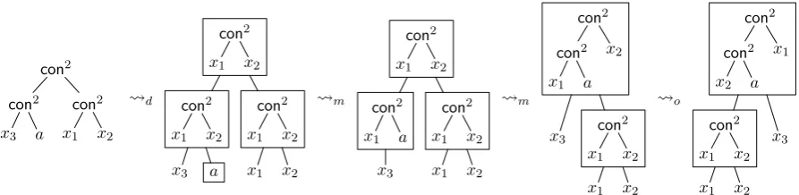
In order to construct h0i(σ) for each symbolσ inξ, we transformtiinto a treet0iwith labels from
C∆i(X)and the same structure asξ. Then we read
offh0i(σ)from the node oft0i that corresponds to theσ-labeled node ofξ. The transformation pro-ceeds as illustrated in Fig. 6: first, we apply the maximal decomposition operation d; it replaces
every label f ∈ ∆i|k by the tree f(x1, . . . , xk),
represented as a box. After that, we keep applying the merge operation m as often as possible; it
merges two boxes that are in a parent-child rela-tion, given that one of them has at most one child. Thus the number of variables in any box can only decrease. Finally, thereorder operation oorders
the children of each box according to the seq of
their variable sets. These operations do not change the variable tree; one can use this to show thatt0i has the same structure asξ.
Thus, if we can find binarization terms, we can construct a binarization ofr. Conversely, for any given binarization(ξ, h01, . . . , h0n)the seman-tic termsh01(ξ), . . . , h0n(ξ)are binarization terms. This proves the following lemma.
Lemma 1 There is a binarization ofrif and only if there are binarization terms ofr.
3.3 Finding binarization terms
It remains to show how we can find binarization terms ofr, if there are any.
Letbi:T∆i(Xk) → P(T∆i(Xk))the mapping
withbi(t) = {t0 ∈ T∆i(Xk) | tandt0 are
equiv-alent, and at each node t0 has at most two chil-dren with variables}. Figure 5b shows some
ele-ments ofb1(h1(α))andb2(h2(α))for our
exam-ple. Termst1, . . . , tn are binarization terms
pre-cisely whenti ∈bi(hi(α))andt1, . . . , tnhave the
same variable tree. Thus we can characterize bi-narization terms as follows.
con2
con2
x3 a
con2
x1 x2
d
con2
x1 x2
con2
x1 x2
x3 a
con2
x1 x2
x1 x2
m
con2
x1 x2
con2
x1 a
x3
con2
x1 x2
x1 x2
m
con2
con2
x1 a
x2
x3 con 2
x1 x2
x1 x2
o
con2
con2
x2 a
x1
con2
x1 x2
x1 x2
[image:6.595.76.523.63.172.2]x3
Figure 6: Transformingt2intot02.
This result suggests the following procedure for obtaining binarization terms. First, determine whether the intersection in Lemma 2 is empty. If it is, then there is no binarization ofr. Otherwise, select a variable treeτfrom this set. We know that there are treest1, . . . , tn such thatti ∈ bi(hi(α))
andv(ti) = τ. We can therefore select arbitrary
concrete treesti ∈bi(hi(α))∩v−1(τ). The terms
t1, . . . , tnare then binarization terms.
4 Effective IRTG binarization
In this section we develop our binarization algo-rithm. Its key task is finding binarization terms t1, . . . , tn. This task involves deciding term
equiv-alence, asti must be equivalent tohi(α). In
gen-eral, equivalence is undecidable, so the task can-not be solved. We avoid deciding equivalence by requiring the user to specify an explicit approxi-mation ofbi, which we call ab-rule. This
param-eter gives rise to a restricted version of the rule-by-rule binarization problem, which is efficiently computable while remaining practically relevant.
Let ∆ be a signature. Abinarization rule (b-rule) over ∆ is a mappingb: ∆ → P(T∆(X))
where for every f ∈ ∆|k we have that b(f) ⊆
C∆(Xk), at each node of a tree inb(f)only two
children contain variables, and b(f) is a regular tree language. We extendbtoT∆(X)by setting
b(xj) = {xj}andb(f(t1, . . . , tk)) = {t[xj/t0j |
1≤j≤k]|t∈b(f), tj0 ∈b(tj)}, where[xj/t0j]
denotes substitution ofxj by t0j. Given an
alge-braAover∆, a b-rulebover∆is calleda b-rule over Aif, for every t ∈ T∆(Xk) and t0 ∈ b(t),
t0andtare equivalent inA. Such a b-rule encodes equivalence inA, and it does so in an explicit and compact way: becauseb(f)is a regular tree lan-guage, a b-rule can be specified by a finite collec-tion of RTGs, one for each symbolf ∈∆. We will look at examples (for the string and tree algebras shown earlier) in Section 5.
From now on, we assume that b1, . . . ,bn are
b-rules over A1, . . . ,An, respectively. A
bina-rization(ξ, h01, . . . , h0n)ofris abinarization ofr with respect to b1, . . . ,bn if h0i(ξ) ∈ bi(hi(α)).
Likewise, binarization terms t1, . . . , tn are
bi-narization terms with respect to b1, . . . ,bn if
ti ∈ bi(hi(α)). Lemmas 1 and 2 carry over to
the restricted notions. The problem of rule-by-rule binarization with respect to b1, . . . ,bn
con-sists in computing a binarization with respect to b1, . . . ,bnfor each suprabinary rule.
By definition, every solution to this restricted problem is also a solution to the general prob-lem. The converse need not be true. However, we can guarantee that the restricted problem has at least one solution whenever the general problem has one, by requiringv(bi(hi(α)) = v(b(hi(α)).
Then the intersection in Lemma 2 is empty in the restricted case if and only if it is empty in the gen-eral case. We call the b-rulesb1, . . . ,b1complete
onGif the equation holds for everyα∈Σ. Now we show how to effectively compute bina-rization terms with respect tob1, . . . ,bn, along the
lines of Section 3.3. More specifically, we con-struct an RTG for each of the sets (i) bi(hi(α)),
(ii) b0i = v(bi(hi(α))), (iii) Tib0i, and (iv) b00i =
bi(hi(α))∩v−1(τ)(givenτ). Then we can selectτ
from (iii) andti from (iv) using a standard
algo-rithm, such as the Viterbi algorithm or Knuth’s algorithm (Knuth, 1977; Nederhof, 2003; Huang and Chiang, 2005). The effectiveness of our pro-cedure stems from the fact that we only manipulate RTGs and never enumerate languages.
The construction for (i) is recursive, following the definition of bi. The base case is a language {xj}, for which the RTG is easy. For the recursive
case, we use the fact that regular tree languages are closed under substitution (G´ecseg and Steinby, 1997, Prop. 7.3). Thus we obtain an RTGGiwith
L(Gi) =bi(hi(α)).
construction. LetGi = (P, p0, R). We define the
mapping vari: P → P(Xk) such that for every
p∈P, everyt∈Lp(Gi)contains exactly the
vari-ables invari(p). We construct it as follows. We
initialize vari(p) to “unknown” for every p. For
every rulep → xj, we setvari(p) = {xj}. For
every rulep→σ(p1, . . . , pk)such thatvari(pj)is
known, we setvari(p) =Sjvari(pj). This is
iter-ated; it can be shown thatvari(p)is never assigned
two different values for the samep. Finally, we set all remaining unknown entries to∅.
For (ii), we construct an RTGG0iwithL(G0i) = b0i as follows. We let G0i = ({hvari(p)i | p ∈
P},vari(p0), R0)whereR0 consists of the rules h{xj}i → {xj} if p→xi ∈R , hvari(p)i →vari(p)(hU1i, . . . ,hUlii)
if p→σ(p1, . . . , pk)∈R,
V ={vari(pj)|1≤j≤k} \ {∅}, |V| ≥2,seq(V) = (U1, . . . , Ul).
For (iii), we use the standard product construc-tion (G´ecseg and Steinby, 1997, Prop. 7.1).
For (iv), we construct an RTG G00i such that L(G00i) =b00i as follows. We letG00i = (P, p0, R00),
whereR00consists of the rules
p→σ(p1, . . . , pk)
if p→σ(p1, . . . , pk)∈R,
V ={vari(pj)|1≤j≤k} \ {∅},
if|V| ≥2, then
(vari(p),seq(V))is a fork inτ .
By a fork (u, u1· · ·uk) inτ, we mean that there
is a node labeleduwithkchildren labeledu1 up
touk.
At this point we have all the ingredients for our binarization algorithm, shown in Algorithm 1. It operates directly on a bimorphism, because all the relevant information about the algebras is captured by the b-rules. The following theorem documents the behavior of the algorithm. In short, it solves the problem of rule-by-rule binarization with re-spect to b-rulesb1, . . . ,bn.
Theorem 3 Let G = (B,A1, . . . ,An) be
an IRTG, and let b1, . . . ,bn be b-rules over A1, . . . ,An, respectively.
Algorithm 1 terminates. Let B0 be the
bimorphism computed by Algorithm 1 on B
andb1, . . . ,bn. Then G0 = (B0,A1, . . . ,An) is
equivalent to G, and G0 is of rank 2 if and only
Input: bimorphismB= (G, h1, . . . , hn),
b-rulesb1, . . . ,bnover∆1, . . . ,∆n Output: bimorphismB0
1: B0 ←(G|
≤2, h1, . . . , hn)
2: forruler:q→α(q1, . . . , qk)ofG|>2do
3: fori= 1, . . . , ndo
4: compute RTGGiforbi(hi(α))
5: compute RTGG0iforv(bi(hi(α)))
6: compute RTGGv forTiL(G0i)
7: ifL(Gv) =∅then
8: addrtoB0 9: else
10: selectt0∈L(Gv)
11: fori= 1, . . . , ndo
12: compute RTGG00i for
13: b00i =bi(hi(α))∩v−1(t0)
14: selectti ∈L(G00i)
15: construct binarization fort1, . . . , tn
16: add appropriate rules toB0
Algorithm 1: Complete binarization algorithm, whereG|≤2andG|>2isGrestricted to binary and
suprabinary rules, respectively.
if every suprabinary rule ofGhas a binarization with respect tob1, . . . ,bn.
The runtime of Algorithm 1 is dominated by the intersection construction in line 6, which isO(m1·
. . .·mn)per rule, wheremiis the size ofG0i. The
quantitymiis linear in the size of the terms on the
right-hand side ofhi, and in the number of rules in
the b-rulebi.
5 Applications
Algorithm 1 implements rule-by-rule binarization with respect to given b-rules. If a rule of the given IRTG does not have a binarization with respect to these b-rules, it is simply carried over to the new grammar, which then has a rank higher than 2. The number of remaining suprabinary rules depends on the b-rules (except for rules that have no bi-narization at all). The user can thus engineer the b-rules according to their current needs, trading off completeness, runtime, and engineering effort.
NP NP DT the
x1:NNP POS
’s
x2:JJ x3:NN
[image:8.595.316.517.61.154.2]−→ dasx2x3derx1
Figure 7: A rule of a tree-to-string transducer.
We show that under certain conditions, our algo-rithm can be used to solve this problem as well. In the following two subsections, we illustrate this for SCFGs and tree-to-string transducers, respec-tively. In the final subsection, we discuss how to extend this approach to other grammar formalisms as well.
5.1 Synchronous context-free grammars
We have used SCFGs as the running example in this paper. SCFGs are IRTGs with two interpre-tations into the string algebra of Table 1, as illus-trated by the example in Fig. 2. In order to make our algorithm ready to use, it remains to specify a b-rule for the string algeba.
We use the following b-rule for bothb1andb2.
Each symbola∈∆i|0 is mapped to the language {a}. Each symbol conk, k ≥ 2, is mapped to the language induced by the following RTG with states of the form[j, j0](where0 ≤ j < j0 ≤ k) and final state[0, k]:
[j−1, j]→xj (1≤j ≤k)
[j, j0]→con2([j, j00],[j00, j0])
(0≤j < j00< j0 ≤k)
This language expresses all possible ways in whichconkcan be written in terms ofcon2.
Our definition of rule-by-rule binarization with respect tob1andb2coincides with that of Huang
et al. (2009): any rule can be binarized by both algorithms or neither. For instance, for the SCFG rule A → hBCDE, CEBDi, the sets v(b1(h1(α)))andv(b2(h2(α)))are disjoint, thus
no binarization exists. Two strings of length N can be parsed with a binary IRTG that represents an SCFG in timeO(N6).
5.2 Tree-to-string transducers
Some approaches to SMT go beyond string-to-string translation models such as SCFG by exploit-ing known syntactic structures in the source or tar-get language. This perspective on translation nat-urally leads to the use of tree-to-string transducers
NP→α(NNP,JJ,NN)
NP
con3
NP
con3
DT the
con0
x1 POS
’s
con0
x2 x3
h1 ←−[α h2
7−→ con
5
[image:8.595.85.278.64.131.2]das x2 x3 der x1
Figure 8: An IRTG rule encoding the rule in Fig. 7.
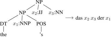
(Yamada and Knight, 2001; Galley et al., 2004; Huang et al., 2006; Graehl et al., 2008). Figure 7 shows an example of a tree-to-string rule. It might be used to translate “the Commission’s strategic plan” into “das langfristige Programm der Kom-mission”.
Our algorithm can binarize tree-to-string trans-ducers; to our knowledge, it is the first algorithm to do so. We model the tree-to-string transducer as an IRTG G = ((G, h1, h2),A1,A2), where A2 is the string algebra, but this time A1 is the
tree algebra shown in Table 1. This algebra has operationsconk to concatenate sequences of trees
and unaryγthat maps any sequence(t1, . . . , tl)of
trees to the treeγ(t1, . . . , tl), viewed as a sequence
of length 1. Note that we exclude the operation
con1 because it is the identity and thus
unneces-sary. Thus the rule in Fig. 7 translates to the IRTG rule shown in Fig. 8.
For the string algebra, we reuse the b-rule from Section 5.1; we call itb2here. For the tree algebra,
we use the following b-rule b1. It maps con0 to {con0}and each unary symbolγto{γ(x
1)}. Each
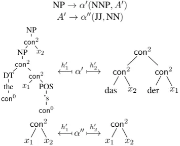
symbol conk, k ≥ 2, is treated as in the string case. Using these b-rules, we can binarize the rule in Fig. 8 and obtain the rules in Fig. 9. Parsing of a binary IRTG that represents a tree-to-string transducer isO(N3·M)for a string of lengthN and a tree withM nodes.
NP→α0(NNP, A0)
A0→α00(JJ,NN)
NP
con2
NP
con2
DT the
con0
con2
x1 POS
’s
con0
x2
h0
1 ←−[α0 h02
7−→
con2
con2
das x2
con2
der x1
con2
x1 x2
h0
1 ←−[α00 h02
7−→ con
2
x1 x2
Figure 9: Binarization of the rule in Fig. 8.
1 1.2 1.4 1.6 1.8 2 2.2 2.4
ext bin
# rules (millions)
rank
[image:9.595.92.270.63.207.2]0 1 2 3 4 5 6-7 8-10
Figure 10: Rules of a transducer extracted from Europarl (ext) vs. its binarization (bin).
5.3 General approach
Our binarization algorithm can be used to solve the general rule-by-rule binarization problem for a specific grammar formalism, provided that one can find appropriate b-rules. More precisely, we need to devise a class C of IRTGs over the same sequence A1, . . . ,An of algebras that
en-codes the grammar formalism, together with b-rules b1, . . . ,bn over A1, . . . ,An that are
com-plete on every grammar in C, as defined in
Sec-tion 4.
We have already seen the b-rules for SCFGs and tree-to-string transducers in the preceding subsec-tions; now we have a closer look at the class C
for SCFGs. We used the class of all IRTGs with two string algebras and in which hi(α) contains
at most one occurrence of a symbol conk for
ev-ery α ∈ Σ. On such a grammar the b-rules are complete. Note that this would not be the case if we allowed several occurrences of conk, as in con2(con2(x1, x2), x3). This term is equivalent
to itself and tocon2(x
1,con2(x2, x3)), but the
b-rules only cover the former. Thus they miss one variable tree. For the termcon3(x1, x2, x3),
how-ever, the b-rules cover both variable trees.
Generally speaking, given C and b-rules b1, . . . ,bnthat are complete on every IRTG in C,
Algorithm 1 solves the general rule-by-rule bina-rization problem onC. We can adapt Theorem 3 by requiring thatGmust be inC, and replacing each
of the two occurrences of “binarization with re-spect tob1, . . . ,bn” by simply “binarization”. IfC
is such that every grammar from a given grammar formalism can be encoded as an IRTG in C, this solves the general rule-by-rule binarization prob-lem of that grammar formalism.
6 Conclusion
We have presented an algorithm for binarizing IRTGs rule by rule, with respect to b-rules that the user specifies for each algebra. This improves the complexity of parsing and translation with any monolingual or synchronous grammar that can be represented as an IRTG. A novel algorithm for binarizing tree-to-string transducers falls out as a special case.
In this paper, we have taken the perspective that the binarized IRTG uses the same algebras as the original IRTG. Our algorithm extends to gram-mars of arbitrary fanout (such as synchronous tree-adjoining grammar (Koller and Kuhlmann, 2012)), but unlike LCFRS-based approaches to bi-narization, it will not increase the fanout to en-sure binarizability. In the future, we will ex-plore IRTG binarization with fanout increase. This could be done by binarizing into an IRTG with a more complicated algebra (e.g., of string tu-ples). We might compute binarizations that are optimal with respect to some measure (e.g., fanout (Gomez-Rodriguez et al., 2009) or parsing com-plexity (Gildea, 2010)) by keeping track of this measure in the b-rule and taking intersections of weighted tree automata.
Acknowledgments
References
Alfred V. Aho and Jeffrey D. Ullman. 1969. Syntax directed translations and the pushdown assembler.
Journal of Computer and System Sciences, 3:37–56.
Andr´e Arnold and Max Dauchet. 1976.
Bi-transduction de forˆets. In Proc. 3rd Int. Coll.
Au-tomata, Languages and Programming, pages 74–86. Edinburgh University Press.
Walter S. Brainerd. 1969. Tree generating regular
sys-tems. Information and Control, 14(2):217–231.
David Chiang. 2007. Hierarchical phrase-based
trans-lation. Computational Linguistics, 33(2):201–228.
Steve DeNeefe and Kevin Knight. 2009. Synchronous
tree-adjoining machine translation. InProceedings
of EMNLP, pages 727–736.
Jason Eisner. 2003. Learning non-isomorphic tree
mappings for machine translation. InProceedings
of the 41st ACL, pages 205–208.
Michel Galley, Mark Hopkins, Kevin Knight, and Daniel Marcu. 2004. What’s in a translation rule? InProceedings of HLT/NAACL, pages 273–280.
Michael Galley. 2010. GHKM rule extractor. http:
//www-nlp.stanford.edu/˜mgalley/ software/stanford-ghkm-latest.tar.
gz, retrieved on March 28, 2012.
Ferenc G´ecseg and Magnus Steinby. 1997. Tree lan-guages. In G. Rozenberg and A. Salomaa, editors,
Handbook of Formal Languages, volume 3, chap-ter 1, pages 1–68. Springer-Verlag.
Daniel Gildea. 2010. Optimal parsing strategies for
linear context-free rewriting systems. In
Proceed-ings of NAACL HLT.
Joseph A. Goguen, Jim W. Thatcher, Eric G. Wagner, and Jesse B. Wright. 1977. Initial algebra
seman-tics and continuous algebras. Journal of the ACM,
24:68–95.
Carlos Gomez-Rodriguez, Marco Kuhlmann, Giorgio Satta, and David Weir. 2009. Optimal reduction of rule length in linear context-free rewriting systems. InProceedings of NAACL HLT.
Jonathan Graehl, Kevin Knight, and Jonathan May.
2008. Training tree transducers. Computational
Linguistics, 34(3):391–427.
Liang Huang and David Chiang. 2005. Better k-best
parsing. InProceedings of the 9th IWPT, pages 53–
64.
Liang Huang, Kevin Knight, and Aravind Joshi. 2006. Statistical syntax-directed translation with extended
domain of locality. InProceedings of the 7th AMTA,
pages 66–73.
Liang Huang, Hao Zhang, Daniel Gildea, and Kevin
Knight. 2009. Binarization of synchronous
context-free grammars. Computational Linguistics,
35(4):559–595.
Donald E. Knuth. 1977. A generalization of Dijkstra’s
algorithm. Information Processing Letters, 6(1):1–
5.
Alexander Koller and Marco Kuhlmann. 2011. A
gen-eralized view on parsing and translation. In
Pro-ceedings of the 12th IWPT, pages 2–13.
Alexander Koller and Marco Kuhlmann. 2012. De-composing TAG algorithms using simple
alge-braizations. InProceedings of the 11th TAG+
Work-shop, pages 135–143.
Philip M. Lewis and Richard E. Stearns. 1966.
Syn-tax directed transduction. Foundations of Computer
Science, IEEE Annual Symposium on, 0:21–35.
Mark-Jan Nederhof. 2003. Weighted deductive
pars-ing and Knuth’s algorithm. Computational
Linguis-tics, 29(1):135–143.
Rebecca Nesson, Stuart M. Shieber, and Alexander Rush. 2006. Induction of probabilistic synchronous tree-insertion grammars for machine translation. In
Proceedings of the 7th AMTA.
Owen Rambow and Giorgio Satta. 1999. Independent parallelism in finite copying parallel rewriting
sys-tems. Theoretical Computer Science, 223(1–2):87–
120.
David J. Weir. 1988. Characterizing Mildly
Context-Sensitive Grammar Formalisms. Ph.D. thesis, Uni-versity of Pennsylvania.
Kenji Yamada and Kevin Knight. 2001. A
syntax-based statistical translation model. InProceedings