Munich Personal RePEc Archive
Predicting the direction of US stock
markets using industry returns
Pönkä, Harri
University of Helsinki, HECER
24 February 2014
Online at
https://mpra.ub.uni-muenchen.de/62942/
öMmföäflsäafaäsflassflassflas
fffffffffffffffffffffffffffffffffff
Discussion Papers
Predicting the direction of US stock markets
using industry returns
Harri Pönkä
University of Helsinki and HECER
Discussion Paper No. 385
September 2014
ISSN 1795-0562
HECER
–
Helsinki Center of Economic Research, P.O. Box 17 (Arkadiankatu 7), FI-00014
University of Helsinki, FINLAND, Tel +358-9-191-28780, Fax +358-9-191-28781,
HECER
Discussion Paper No. 385
Predicting the direction of US stock markets
using industry returns*
Abstract
In this paper, we examine the directional predictability of excess stock market returns by
lagged excess returns from industry portfolios and a number of other commonly used
variables by means of dynamic probit models. We focus on the directional component of
the market returns because, for investment purposes, forecasting the direction of return
correctly is presumably more relevant than the accuracy of point forecasts. Our findings
suggest that only a small number of industries have predictive power for market returns.
We also find that the binary response models outperform conventional predictive
regressions in forecasting the direction of the market return. Finally, we test trading
strategies and find that a number of industry portfolios contain information that can be
used to improve investment returns.
JEL Classification:
C25, C53, C58, G17
Keywords:
industry excess return, sign prediction, probit model, forecasting
Harri Pönkä
Department of Political and Economic Studies
University of Helsinki
P.O. Box 17 (Arkadiankatu 7)
FI-00014 University of Helsinki
FINLAND
e-mail: [email protected]
1. Introduction
There is a vast literature in financial economics focusing on the prediction of stock returns using publicly available information. The topic is of interest from many perspectives. From an empirical point of view, these studies provide information on the factors driving stock markets. The potential for increased returns through better forecasts has kept the topic current among financial practitioners. From a theoretical perspective, studies on stock return forecasting can be seen as tests of asset pricing theories. For a comprehensive and up-to-date overview of the literature on the different variables, methodologies, and theories used in the research on stock return predictability, we refer to Rapach and Zhou (2013).
As a reaction to prevailing anomalies in stock markets, there is a large number of studies that relax the strict assumptions of rationality, perfect markets, and unlimited information processing power of investors. Among these studies a growing literature on behavioural theories aim to explain some aspects of investor behaviour. One of these is the unified theory of underreaction, momentum trading, and overreaction in asset markets, proposed by Hong and Stein (1999). This theory is based on the idea of gradual diffusion of information across investors, which causes prices to underreact in the short run, making it possible for momentum traders to profit from trend chasing. Moskowitz and Grinblatt (1999) study the momentum effect of industries and find that investment strategies based on buying previously profitable industries and selling previously losing industries turn out to be highly profitable. Focusing on industries is potentially an interesting way to study the gradual diffusion of information and momentum effects, since investors with limited information processing capabilities might not be able to follow markets as a whole, but instead focus on a few industries. This issue is addressed in by Hong, Torous, and Valkanov (2007), who study the predictive ability of industry portfolios for excess stock market returns. Their findings from predictive regressions suggest that a number of industries lead the stock markets in the US and eight largest non-US markets, which can be seen as evidence in favor of information diffusing slowly within markets.
The purpose of this study is to extend the research on the predictive power of industry portfolio returns on excess stock market returns. However, in contrast to the previous literature, we do this by examining whether thedirection
of stock markets can be predicted by lagged returns of industry portfolios. Our main motivation is to see whether the previous findings of Hong et al. (2007), among others, hold in the dynamic probit models of Kauppi and Saikkonen (2008). These models are similar in spirit to the autologistic models of Rydberg and Shephard (2003), and Anatolyev and Gospodinov (2010).
We focus on the directional component of the excess market returns because, based on a number of previous empirical results, it can be argued that for investment purposes predicting the direction of return correctly is more relevant than the accuracy of point estimates. In particular, there is some evidence that classification-based models, such as binary response models outperform traditional predictive regression models (also referred to as ’level models’ below) in terms of profitability of investment strategies built on their forecasts (see Leung, Daouk, and Chen (2000)). The dynamic probit models have been used in a similar application by Nyberg (2011), who finds that six-month-ahead recession forecasts perform well as predictors of the direction of the stock market in the US.
Our in-sample results indicate that only two to eight out of 34 industries lead the stock market in our application. Hence, we find only weak evidence in favor of diffusion of information across asset markets. On the other hand, our findings suggest that information from certain industry portfolios is indeed useful in out-of-sample forecasting, and may be used to increase profitability of trading strategies.
This paper is organized as follows. In the following section, we summarize findings of Hong et al. (2007) and related research. In Section 3, we discuss the methodology, and in Section 4 we introduce the data. We are primarily interested in testing for the presence of gradual diffusion of information across markets, and this is the purpose of the we study in-sample analysis in Section 5. In addition, we are interested in comparing the forecast performance of the predictive regressions and dynamic probit models. This is the focus of Section 6 where we report the out-of-sample forecasting results. In Section 7, we conclude and discuss possible extensions.
2. Previous literature
As pointed above, the study most closely related to ours, is that of Hong et al. (2007), who study the predictive ability of industry portfolio returns for monthly US stock market returns in 1946-2002. They also examine the corresponding predictive relationship in Japan, Canada, Australia, the UK, Netherlands, Switzerland, France, and Germany for a shorter period running from 1973 to 2002. The hypothesis behind the analysis is that the information originating from certain industries, in general, diffuses to the stock market only with a lag. This hypothesis is based on the assumptions that news travels slowly across markets, and that investors have limits to the amount of information they can process, meaning that most of them can only follow a limited amount of industries.
Hong et al. (2007) consider the following predictive regression for each industry portfolio separately:
REt=αi+λiRi,t−1+AiZt−1+ei,t, (1)
whereREtis the excess return on the market portfolio at timet,Ri,t−1is the excess return on industry portfolioiat
timet−1,Zt−1 is a vector of control variables, andei,tis the error term. The control variables are used as proxies
for time-varying risk and include variables, such as inflation and the lagged excess market returnREt−1. Model (1)
leads to two testable hypotheses of the predictive power of industry portfolios for the whole stock markets and market fundamentals. With the main emphasis being on the US markets, they find that over the period 1946-2002, the excess returns in 14 out of 34 industries, including commercial real estate, petroleum, metal, retail, financial, and services, can predict market movements by one month. A number of other industries, such as petroleum, metal, and financial, can forecast the market as far as two months ahead. Even after including a variety of well-known proxies for risk and liquidity as well as lagged market returns in the vectorZt−1, the predictability of the market by these 14 industry
portfolios remains statistically significant.
A secondary goal of Hong et al. (2007) was to analyze the hypothesis that the ability of an industry to forecast the market is related to its ability to forecast changes in market fundamentals such as industrial production growth or changes in other indicators of economic activity. Their results on the predictability of industrial production growth by industry returns indicate that the same industries that have predictive power for the stock market in the US also predict industrial production growth. In nine industries predictability turns out to be statistically significant at the 5 percent level and in a further twelve at the 10 percent level. The mining, petroleum, and metal industries forecast the market and industrial production with a negative coefficient, whereas industries such as retail and financial have a positive coefficient.
Besides Hong et al. (2007), the predictive power of asset portfolios on aggregate market returns and other eco-nomic variables has been discussed in a number of studies, albeit the literature is scant. Lamont (2001) studies economic tracking portfolios, which are portfolios of assets that lead economic variables. His results suggest that monthly returns on stocks and bonds are useful in forecasting post-war US output, consumption, labor income, infla-tion, stock returns, bond returns, and Treasury bill returns. These findings are in line with those of Hong et al. (2007) in that industry portfolios can track both excess market returns as well as economic variables, such as inflation, growth in industrial production, and consumption growth. In a study focusing on a single industry, Cole, Moshirian, and Wu (2008) study the relationship between the financial industry stock returns and future GDP growth. They analyze data from 18 developed and 18 emerging markets using dynamic panel techniques and report a positive significant rela-tionship between bank stock returns and economic growth. Furthermore, Menzly and Ozbas (2010) study the gradual diffusion of information in stock markets by analyzing the cross-predictability of stock returns from industries that have a supplier-customer relationship.
3. Methodology
In this paper, our aim is to predict the direction of US stock markets using lagged excess returns from industry portfolios. To this end, we use two types of models. Predictive regression models, such as the one presented in equation (1), are commonly used to study the statistical significance of potential predictors of excess stock market returns. We also employ these models in order to compare the directional predictive power these so-called level mod-els with dynamic binary response modmod-els. In this sense, we follow the work of Leung et al. (2000) who compare classification-based models and predictive regressions in forecasting stock indices. However, our work differs from theirs by focusing on the potential predictive power of industry returns and using dynamic probit models proposed by Kauppi and Saikkonen (2008), whose empirical application was related to forecasting US recessions. Given the binary nature of the NBER classification of expansions and contractions, recession forecasting has been a popular application of these models (see e.g. Nyberg (2010) and Ng (2012)).
Our application is somewhat different, as we observe the actual values of returns and not only the direction. How-ever, previous findings have suggested that the directional predictability is more important than mean predictability for building successful trading strategies. Christoffersen and Diebold (2006) show that given the volatility dynamics in stock returns, one can find sign predictability even in the absence of mean predictability. Nyberg (2011) has a similar application to ours as he uses dynamic probit models to forecast the direction of the US stock market. A main focus in his paper is to use recession forecasts as an explanatory variable in the forecast for the sign of the excess stock return and to compare different model specifications in this framework. The main difference to our paper is the use of different predictors.
3.1. Binary Response Models
A key idea in our application of the binary response models is that the excess stock market return is transformed into a binary sign return indicatorytthat is used as the dependent variable:
yt=
1,if the excess return is positive,
We denote a vector of explanatory variables asxt, which in our case includes returns from industry portfolios and
commonly used market predictors. These variables will be discussed in more detail in Section 4. The information set at timetis given byΩt=σ[(ys,xs),t>s]. Now,ytconditional onΩt−1, follows a Bernoulli distribution
yt|Ωt−1∼B(pt). (3)
If we denote the conditional expectation and probability given information setΩt−1asEt−1(·) andPt−1(·) respectively,
we may define
pt=Et−1(yt)=Pt−1(yt=1). (4)
Moreover, to specify the conditional probability of positive excess stock returnspt, we form a probit model
pt= Φ(πt), (5)
whereΦ(·) is the cumulative distribution function of the standard normal distribution andπtis a linear function of the
variables inΩt−1. Assuming a logistic distribution instead would yield a logit model.
To complete the model, the basic and most commonly used specification is the static probit model, whereπtis
specified as
πt=ω+x′t−1β, (6)
wherext−1 includes lagged values of the explanatory variables andωis a constant term. The static model (6) may
also be extended in various ways. One option is to include lagged values ofyt, producing a dynamic probit model
πt=ω+δ1yt−1+x′t−1β. (7)
It is important to note that in this paper, we restrict ourselves to the first-order case presented in model (7), as preliminary findings suggest that higher-order lags ofytdo not add predictive power.
Alternatively, lagged values of the linear functionπtmay be added into the model to introduce an autoregressive
structure. Augmenting the model by first-order lags ofπt, we get a first-order autoregressive probit model
πt=ω+α1πt−1+x′t−1β. (8)
Finally, including the lagged values of bothytandπtyields a dynamic autoregressive probit model
πt=ω+α1πt−1+δ1yt−1+x′t−1β. (9)
The parameters of models (6)-(9) can be estimated using maximum likelihood (ML) methods. For more details on the estimation and the calculation of Newey-West type robust standard errors, we refer to Kauppi and Saikkonen (2008).
3.2. Goodness-of-fit Measures and Statistical Tests
As we employ different types of models, i.e. binary and continuous dependent variable models, in both in-sample estimation and out-of-sample forecasting, we need a number of different measures to evaluate the statistical fit and predictability of our models. For the predictive regressions like (1), we evaluate the in-sample fit by the commonly used adjusted-R2measure. For the dynamic probit models, we employ similar goodness-of-fit measures as Nyberg (2011). The main measure used to evaluate the in-sample goodness-of-fit of the probit models is the adjusted
pseudo-R2measure of Estrella (1998), defined as
ad j.psR2=1−(logLu−logLc)−(2/T)logLc×(T −1)/(T−k−1), (10)
wherelogLu andlogLc are the maximum values of the estimated constrained and unconstrained log-likelihood
functions respectively, T is the length of the sample, andk is the number of explanatory variables. We use the adjusted form of the measure since it takes into account the trade-offbetween improvement in model fit and the loss in degrees of freedom. It is worth noting that, although it is on a similar scale as the adjusted-R2generated in ordinary
least squares (OLS) regression, these two measures are not directly comparable. For the probit models we also report the Bayesian information criterion (BIC), which is typically used for model selection purposes.
Although in in-sample estimation we are interested in the statistical fit of the models, the main focus is on studying the statistical significance of the coefficients for industry portfolios. In out-of-sample forecasting in Section 6, we focus on the comparison of the sign forecasting performance of each model. In our application, the results produced by the probit models are probability forecasts of positive excess market returns in a given period. Therefore, we need to convert these probabilities into sign forecasts based on a threshold value. In other words, the sign forecast is defined as
ˆ
yt=1[pt>c], (11)
where1[·] denotes an indicator function and pt is given in (4) and (5). In this study, we use a natural threshold of
c=0.50, which is also the most commonly used one in the literature. Similarly, we need to convert the results from predictive regressions into sign forecasts. This is done in the same way as for the realized excess market returns in (2). In other words, if ˆREtin model (1) is positive, we get a signal forecast ˆyt=1.
Based on the threshold and the obtained forecasting signals, we report the success ratio of our forecasts, denoted as SR. This ratio can be expressed as
S R= yˆ
uu+yˆdd
ˆ
yuu+yˆdu+yˆud+yˆdd, (12)
where the forecasts are classified as
ˆ
yuu=
T X
t=1
1[ˆyt=1,yt=1],
ˆ
yud=
T X
t=1
1[ˆyt=1,yt=0],
ˆ
ydu=
T X
t=1
1[ˆyt=0,yt=1],
ˆ
ydd=
T X
t=1
1[ˆyt=0,yt=0],
In these expressions ˆytis the forecast ofyt,uis an upward signal anddis a downward signal.
Pesaran and Timmermann (1992) have proposed a statistical test of directional accuracy (DA) that measures whether the value of SR is significantly different from the success ratio that would be obtained when the realized valuesytand the forecasts ˆytare independent. A detailed description of the test statistic is also presented by Granger
and Pesaran (2000), and following their notation, the test statistic can be written as
DA=
√
T(HR−FR)
Pˆy(1−Pˆy)
¯
y(1−y¯)
1/2
(13)
where ¯yis theT-month sample average of the binary variableyt, the hit rateHR =
ˆ
yuu
ˆ
yuu+yˆdu, and false rateFR =
ˆ
yud
ˆ
yud+yˆdd. Finally, ˆPy=¯zHR+(1−z¯)FR. The test statistic (13) has the asymptotic standard normal distribution under
the null hypothesis thatytand ˆytare independently distributed.
As an extension of the test statistic (13), Pesaran and Timmermann (2009) have recently suggested a new test of predictability that is better suited for market timing when there is serial correlation inyt and the signal forecasts ˆyt.
This test statistic can be written as
PT =(T−1)(S−yy1,wSyyˆ,wSy−ˆyˆ1,wSyyˆ,w)∼χ21, (14)
where
Syy,w=(T −1)−1Y′MwY,
Syˆyˆ,w=(T−1)−1Yˆ′MwYˆ,
Syyˆ,w=(T −1)−1Yˆ′MwY,
Syyˆ,w=(T−1)−1Y′MwYˆ,
Mw=IT−1−W(W′W)−1W′,
W =(τT−1,Y−1,Yˆ−1),
andY = (y2, ...yT)′,Yˆ = (ˆy2, ...yˆT)′,Y−1 = (y1, ...yT−1),Yˆ−1 = (ˆy1, ...yˆT−1), and τt is a (T −1)×1 vector of ones.
3.3. Trading strategies
In applications focusing on excess returns, the market timing ability of models is commonly tested using trading strategies based on their out-of-sample forecasts. This is motivated by Leitch and Tanner (1991), who argue that models performing well according to statistical criteria might not be profitable in market timing. In our paper, we will consider simple trading strategies similar to those in Leung et al. (2000) and Nyberg (2011). This will allow direct comparison of trading returns between the conventional predictive regressions and the probit models. These returns may also be compared to ones obtained by using common benchmarks, such as the buy-and-hold trading strategy.
For our trading strategy, we assume that an investor decides a financial asset allocation at the beginning of each month. The choice of assets consists of stocks (risky asset) and the one-month T-bill rate (risk-free asset). The investment decision is based on the various forecasting models. If the directional forecast ˆyt=1, the investor invests
only in stocks. In our case this is the CRSP market portfolio, which we assume tradable through a hypothetical index fund. If the forecast model predicts a downward movement in stock markets ˆyt =0, the investor allocates the whole
portfolio to one-month T-bills. In the basic setup we assume zero transaction costs and no short-sales for the sake of simplicity, but we also perform robustness checks allowing for both of these additional features.
When studying the profitability of investment strategies, one should also take into account the riskiness of the portfolios. The Sharpe ratio (1966, 1994) is the most commonly used measure of risk adjusted return in finance. It is a convenient tool in ranking portfolio performance, but its numerical value is difficult to interpret. It describes the amount of excess return that the investor receives for the added volatility from holding a more risky asset. In this study, the ex-post Sharpe ratio is defined as
S = (rp−rf)
σp
, (15)
whererpandσpare the return and standard deviation of the investment portfolio, andrfis the risk-free return.
4. Data
There has been abundant research on economic and financial variables that can be used as predictors for excess stock returns. In terms of data, we start off by using a similar set of variables as Hong et al. (2007). We also entertain alternative predictive variables based on previous studies, such as Goyal and Welch (2008), who consider a comprehensive set of other potential predictors.
The stock market data are monthly returns from the Center for Research in Security Prices (CRSP), available at Kenneth French’s data library1. We use monthly data ranging from 1946M1 to 2012M12. The dataset for the US
stock market return is the excess market return on the value-weighted market portfolioREt, which is defined as the
difference between the market returnRMtand the risk-free rateRFt(i.e.REt=RMt−RFt). The data for the industry
portfolios include monthly excess returns on 34 value-weighted industry portfolios similar to Hong et al. (2007). The data for the Agriculture, Forestry, and Fishing (AGRIC) and Real Estate (REIT) industries are only available from 1965M01 and 1972M01 onwards, respectively. Models including these portfolios are therefore estimated for a shorter sample.
In addition to stock returns, we use data for selected market fundamentals obtained from the St. Louis Federal Reserve Economic Data (FRED) library2. We include the growth rate of the consumer price index (CPI) as well as the default spread (DSPR) defined as the difference between BAA- and AAA-rated bond yields. The market dividend yield (MDY) is obtained for the S&P500 companies, and it is defined as the ratio of annual dividends to current prices. Finally, we include a measure of monthly market volatility (MVOL) calculated from daily data on the market returns, in the same way as in French, Schwert, and Stambaugh (1987). We also consider other possible variables, such as the term spread (TERM) and the change in the 3-month T-bill rate (3MTH), which have been found useful predictors of excess stock returns in previous studies (e.g. Fama and French, 1989). Table 1 provides the details of the 34 industries used in our study and includes the means and standard deviations of the monthly returns.
5. In-sample Results
In the in-sample estimations, we experiment with a number of different explanatory variables and model spec-ifications. We restrict ourselves to using only the first lags of the industry returns and other explanatory variables, which is typical in this kind of predicting exercises. In order to keep the models relatively parsimonious, we set the maximum number of explanatory variables at six. Due to the large number of different model specifications, we only report the most relevant results. All the other results are available upon request. Specifically, we will present results
1http://mba.tuck.dartmouth.edu/pages/faculty/ken.french/index.html
2http://research.stlouisfed.org/fred2/
from models including the same explanatory variables as Hong et al. (2007); the lagged excess market return (RE), consumer price inflation (CPI), default spread (DSPR), market dividend yield (MDY), and market volatility (MVOL). In addition, we report the results of an alternative specification that yields the best in-sample fit among models with at most six explanatory variables. We also consider three different in-sample periods in order to study whether the results vary in time. We estimate models for each of the 34 industries separately.
Our full sample runs from 1946M1 to 2012M12. In order to compare our results with those of Hong et al. (2007), we also use a subsample that covers 1946M1-2002M12. Finally, as we will perform out-of-sample forecasting in the next section, we will also study results for a shorter in-sample period running from 1946M1-1985M12. The use of different subsamples will allow us to study the time-variability in the explanatory power of the models in general as well as the potential changes in the coefficients of predictive variables.
5.1. In-sample Results from Predictive Regressions
We start by studying results of predictive regressions in the style of Hong et al. (2007). As discussed above, we use a similar set of predictive variables, but extend their sample size by ten years, i.e. until the end of 2012. By doing this we are able to study whether there has been substantial changes in the predictive power of industry returns on market returns over the last decade. Some differences in results could be expected since the latter part of the sample contains the recent financial crisis period. We report the results for the predictive regressions including the industry METAL in Table 2 as an illustration of our findings, as it is among the industries with stronger predictive ability. The METAL portfolio is a natural choice in the sense that Hong et al. (2007) also use it to illustrate their results. We do, however, also report the industry coefficients and adjusted-R2values for all of the 34 industries in the first column of
Table 5.
Our results indicate that the default spread and market volatility have low predictive power. Thus, we also exam-ine different specifications of the models with fewer explanatory variables and some alternative predictors. Previous studies have suggested that the term spread and short term interest rates are useful predictors of the excess stock market returns. As it turns out, we find the best overall fit measured by the adjusted-R2when we replace the default
spread and the market volatility with the term spread (TS) and the first difference of the 3-month T-bill (3MTH) rate. As indicated in Table 2 for the model with the METAL portfolio, the in-sample fit of the model is improved rather significantly by this change. At the same time the statistical significance of the METAL-variable is reduced, as can be seen by comparing the first two columns. We also considered models with three and five predictors, but in general the six variable models produce the best fit.
Another key issue that can be seen in Table 2 is that the model fit in terms of the adjusted-R2is inferior for the longer samples. Compared to the shortest sample period used, the adjustedR2is almost double that of the full sample. This indicates that the predictability of excess stock market returns seems to vary substantially in time, which is an issue discussed in a number of papers, including Timmermann (2008).
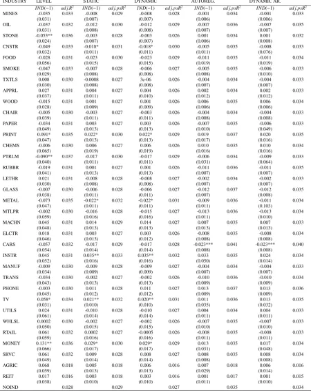
Since the alternative specification that includes TS and 3MTH as explanatory variables generally produces a higher in-sample fit, we focus on results of these models. As can be seen from the first column of Table 5, our re-sults indicate that there are only three out of 34 industries, including Nonmetalic Minerals Except Fuels (STONE), Petroleum and Coal Products (PTRLM), and Finance, Insurance, and Real Estate (MONEY), that have statistically significant coefficients at the 5% level. Compared to the 12 out of 34 industries found by Hong et al. (2007), this is a clear reduction. At the 10% significance level, there are a further two industries that show predictive power for the market return. These industries are PRINT and TV. Hence, in total we find only five industries that show some level of statistical significance, compared with 14 reported by Hong et al. (2007). Using the same explanatory variables as the original specification in Hong et al. (2007), the number of statistically significant industry coefficients (at least at the 10% level) increases to 8. The recent financial crisis during the recent years is one potential explanation to the differences in results. It is also worth noting that there have been some changes in the composition of the industry portfolios in Kenneth French’s database, which may have lead to changes in the results.
To see if potential data revisions or changes in the industry portfolios have altered our results, we also replicate the predictive regressions using the same sample as Hong et al. (2007). Our findings are somewhat different from theirs as we find that using the currently available datasets and our alternative specification, the returns on only two indus-try portfolios show statistically significant predictive ability for the excess market return at the 5% level and further four at the 10% level. As mentioned, there are a number of potential reasons for this difference. In addition to data revisions, one potential source of differences comes from the calculation of the standard errors. In this paper, we use Newey-West type standard errors as in Kauppi and Saikkonen (2008), while in Hong et al. (2007) the standard errors are formulated to take into account the potential correlation of the residuals across industries. It is also noteworthy that the results based on the exact same predictors as Hong et al. (2007) are somewhat stronger in terms of statistical significance of industry coefficients. This might imply that the lagged term structure (TS) and lagged three-month T-bill rate (3MTH) capture some of the same information as the industry portfolios.
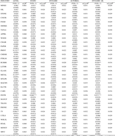
predictive ability for the excess market return at the 5% level and a further three at the 10% level. These results for all industries are presented in the appendix (Table 9). In general, the results for the predictive regressions do not change much in different samples in terms of which industry portfolios have predictive power, although this is the case for METAL in Table 2.
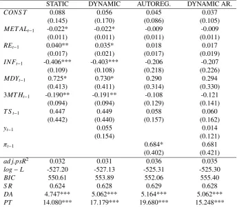
5.2. In-sample Results From Dynamic Probit models
With the static probit model (6) for the full sample 1946M1-2012M12, we find that two (of the 34) industry co-efficients show statistically significant predictive power at the 5% level. These industries are INSTR and TV. Further four industries show statistical significance at the 10% level; METAL, CNSTR, PRINT, and MONEY. All except INSTR are among the same industries that also Hong et al. (2007) reported to have predictive power. However, in general, our results do appear to be somewhat weaker in the sense that we find less evidence on the explanatory power of industry returns. We report the results for the static probit models including the industry METAL in Table 3. As in the case of the predictive regressions, the model that includes TS and 3MTH has a better in-sample fit than the model including DSPR and MVOL, measured in this case with the adjusted pseudo-R2. For this reason, we focus
mainly on the results of this specification, although evidence for the explanatory power of industry portfolio returns would be slightly stronger if we would use the same set of explanatory variables as Hong et al. (2007). It should also be pointed out that for the sample period 1946M1-1985M12 only two of the 32 industry coefficients are statistically significant, so the sample period does have an impact on these results (see Table 9). Differences in results between sample periods can also be seen in Table 3 in the case of the model with the METAL portfolio.
The signs of the statistically significant industry coefficients in the static probit models are similar to those ob-tained using predictive regressions. These signs can also be given economic interpretations. Although we will not focus on this aspect in detail, it is still noteworthy that, e.g., the returns in the METAL industry portrays the com-modity prices of metal, which are typically countercyclical. Since the relationship between business cycles and stock markets is typically positive, the estimated negative sign makes economic sense. On the other hand, industries such as PRINT and MONEY are commonly thought of as being procyclical, which is also in line with our results.
The in-sample estimation results of the dynamic probit models are rather interesting. Table 4 contains results obtained with the model including the METAL portfolio as an explanatory variable, while in table 5 we report the results for the remaining industries. The results of the so-called dynamic specification (7) are almost identical to those of the static probit model (6). The reason for this is most likely that we already have the lagged excess market return
REt−1in the set of control variables, so the lagged sign of the excess market returnyt−1turns out to be statistically
insignificant. We also entertained models that excludedREt−1, but the overall in-sample fit was considerably lower.
The results from autoregressive probit models (8) indicate that none of the coefficients for the industry returns are any longer statistically significant when we include the first lag ofπt in the model. However, the coefficients
of the lagged pi’s are, in general, highly statistically significant, and the pseudo-R2values do increase substantially
compared with the static (6) and dynamic (7) specifications. The results of the dynamic autoregressive probit models (9) are rather similar to those of the autoregressive probit models. In general, the adjusted pseudo-R2values are rather low, generally varying between 1.5% and 4%. Overall, low explanatory power is typical in models for predicting stock returns. For instance, Rapach and Zhou (2013) mention that an upper bound for the predictability of stock returns (usingR2) could be evaluated to be around 8%, which is still too loose to be binding in empirical applications. Overall, our in-sample results indicate that returns from only a few industry portfolios are useful predictors of the excess market returns. However, the results of theDAandPT tests suggest that the signs of the excess market returns are predictable. The findings presented in Tables 3 and 4 indicate that we reject the null of no predictability in each of the specifications (including the METAL portfolio).
Compared with Hong et al. (2007), we find less evidence in favor of the hypothesis that information diffuses slowly across markets. Goyal and Welch (2008) note that it is not uncommon in studies focusing on predicting the equity premium that following studies using similar variables have found weaker or contradictory results, and above we have discussed a number of potential reasons for this in this study. Although our results are not very strong in terms of the in-sample predictive ability of excess industry returns, we have found interesting results on the diff er-ences between predictive regressions and dynamic probit models. In the next section we make out-of-sample forecasts comparing the models presented above, paying attention especially on the industries that had statistically significant in-sample predictive power.
6. Out-of-sample results
In this study, the out-of-sample period runs from 1986M1 to 2012M12, including 324 observations. We make one-month-ahead sign forecasts of the of excess stock market returns. We employ an expanding (recursive) estima-tion window when constructing the out-of-sample forecasts. Our in-sample results indicated that the predictive power of the models has changed in the last 26 years, so the choice of the out-of-sample period may have an effect on the
results. The issue of splitting the data into estimation and evaluation periods is discussed e.g. by Hansen and Tim-mermann (2012), who demonstrate that out-of-sample forecast results may be highly dependent on the sample split, especially if the evaluation sample is left short. Therefore, to maximize the power of the forecast evaluation tests, we have selected a rather long out-of-sample period.
The out-of-sample forecasting performance is analyzed using a number of different measures. We find that the out-of-sample pseudo-R2 measures are in many cases negative for the static probit model, which is an implication
of a relatively low level of predictability, commonly found in models for excess stock returns. This is an issue that has been discussed in a number of previous papers. It is not uncommon that forecasting results deemed statistically insignificant by ’traditional’ statistical measures are still economically significant (see e.g. Cenesizoglu and Timmer-mann, 2012). Therefore, we employ a number measures, such as the success ratio (SR) and both of the Pesaran and Timmermann (1992, 2009) tests to evaluate the out-of-sample performance of our models.
Again, we illustrate our findings using the model with the METAL portfolio included as an explanatory variable. These results are reported in Table 6. The results indicate that the best out-of-sample performance among the probit models is obtained with the dynamic version of the model, with 64.5% correct forecasts. The static probit model pro-duces rather similar results (64.2%), but the autoregressive and especially the dynamic autoregressive model perform worse, with 61.7% and 59.9% forecast accuracies, respectively. This shows that good in-sample fit does not necessar-ily imply good performance out-of-sample, as the autoregressive probit model was superior to the static and dynamic models evaluated by the in-sample adjusted pseudo-R2. The predictive power of the static and dynamic probit models
is also statistically significant even at the 1% level according to the two forms of the Pesaran and Timmermann test in equations (13) and (14). Finally, it is noteworthy that the success ratio obtained for the predictive regression model is 58.6%, which is lower than for any of the probit models (see the first column in Table 6). One potential reason for the inferior performance is that predictive regression models have not been specifically designed for directional forecasting.
The last two columns in Table 6 contains the results for the trading strategies based on forecasts of the correspond-ing models. As mentioned above, includcorrespond-ing tradcorrespond-ing strategies allows us to compare findcorrespond-ings uscorrespond-ing both statistical and economic measures of forecast accuracy. We report the annual returns on each trading strategy, and in order to take into account the level of risk associated, we also report the Sharpe ratio (15). Results are generally in line with the findings based on the success ratio and the DA and PT test statistics. We find that the annual return for the buy-and-hold strategy is 9.75% for the period 1986M1-2012M12. The return based on the directional forecasts from the predictive regression model including the METAL portfolio is actually slightly lower than this (9.65%). On the other hand, the return from the strategy based on the static probit model is 12.29%, which is clearly higher than either of the above. In comparison, a static probit model excluding the industry return yields an annual return of 11.60%. Furthermore, the return from the dynamic probit model including the METAL portfolio yields the highest investment return (12.62%), whereas the returns from the autoregressive (10.63%) and the dynamic autoregressive probit (10.13%) models are slightly lower than those from the static model. The risk-adjusted returns measured by the Sharpe ratio rank the strategies in the same order as the unadjusted returns, as the standard deviations of the returns from the trading strategies are rather similar to one another.
We also consider a trading strategy where we include trading costs of 0.5%. This cost is charged each time the contents of the investment portfolio is switched from stocks to the risk-free rate, and vice versa. Including transaction costs reduces the returns from the trading strategies, but does not change the findings significantly. The returns from the dynamic and static probit models remain considerably higher than the return from the buy-and-hold strategy. We also consider the use of short sales instead of using the risk-free rate as the alternative investment. This amplifies the differences between the trading strategies, but does not change the general findings. These results are available upon request.
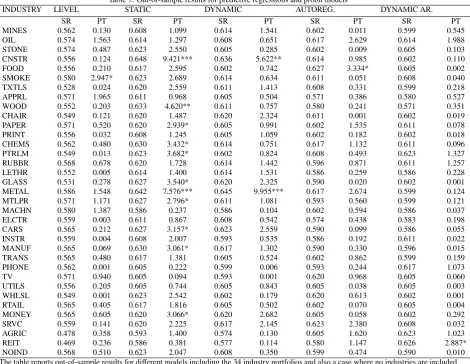
The results for the models with the different industry portfolios are available in Table 7. The findings are generally rather similar to those for the model with the METAL portfolio in Table 6. The static probit model is most commonly the best among the probit models according to the SR measure. In three out of 34 cases the static models get a value of the PT test statistic (14) that is statistically significant at least at the 5% level and in further eight cases at the 10% level. The dynamic probit models perform considerably worse although they outperform the predictive regressions.
The results in Tables 6 and 7 may also be compared to results from models that do not include industry portfolios as predictors. With the static probit model this specification produces a success ratio of 62.3%, which is somewhat lower than that of the model with the METAL portfolio in Table 6, but higher than those of the majority of other industries reported in Table 7.
The dynamic probit models do not perform quite as well as in the case of the model including the METAL port-folio return in Table 6, but they still outperform the autoregressive, dynamic autoregressive, and level models. In most cases the models including the return on either the CNSTR or WOOD industry outperform the models with no industry returns included (NOIND). Results for the models with the PTRLM industry return are more mixed.
Overall, we can conclude that as far as trading strategies are concerned, relying on the static probit model is gen-erally the best option. Some industries, such as METAL and CNSTR do seem to contain information that can help gain higher returns in the out-of-sample period. This suggests that we should put a great emphasis on model selection when choosing the optimal industry portfolio as a predictor of the future sign of the excess market return. Our results for economic and statistical measures of forecast accuracy are also similar to one another.
7. Conclusion and possible extensions
The aim of this paper has been to study the predictive ability of industry portfolios for excess US stock market returns. We have employed conventional predictive regressions (1) and dynamic probit models (6)-(9) to study the topic both in- and out-of-sample, and add to the literature by focusing on the directional component of the excess market returns. In our in-sample estimation, we find that a number of industries lead the stock markets by one month, the exact number depending varying between different model specificcations used. However, contrary to previous findings by Hong et al. (2007), we find somewhat less evidence to support the gradual diffusion of information across markets, especially when we use the model specification that yields the highest in-sample fit. In addition to studying the predictive ability of industry portfolios, we also provide new results on the differences between in-sample esti-mation and out-of-sample forecasting. Our out-of-sample results indicate that the direction of excess market returns are predictable, and that industry portfolios do contain information that can be used for this purpose. One of our key findings is that the dynamic probit models produce more accurate out-of-sample forecasts of the direction of the excess stock market returns than the conventional predictive regression model, which clearly supports the use of these models. Our findings also indicate that although the probit model including an autoregressive structure (8) yields the best in-sample fit, the more parsimonious static probit model (6) performs better out-of-sample. Our findings are sub-stantiated by employing both statistical and economic measures of forecast accuracy, as they yield remarkably similar results in our application. This is an interesting result in itself because, for example, Cenesizoglu and Timmermann (2012) have suggested that the results from statistical tests and investment strategies are not always in line with each other.
In terms of profitability of trading strategies, we find that especially the metal and construction industry portfolios contain information that could be used to obtain higher investment returns during the out-of-sample period 1986M01-2012M12. Models including the excess returns of these two industry portfolios were also the best according to statistical criteria. How the information included in the industry portfolios would actually convert into exploitable arbitrage opportunities in the future is another issue.
This paper could be extended in a number of ways. One possibility is to use industry portfolio returns in excess of market returns as explanatory variables. A radically different approach would be the use of an indicator for bear and bull markets as the dependent variable instead of the direction of the monthly market movements, as is done by Nyberg (2013). The motivation for predicting these long periods of positive and negative returns is based on the idea that different types of investment opportunities are profitable during these regimes, and identifying the shifts from one regime to another is useful information for investors. Identifying turning points between bear and bull markets is closely related to the identification of business cycle turning points, for which the business cycle indicator of the National Bureau of Economic Research (NBER) is the most commonly used benchmark in the U.S., and it is used in most of the studies focusing on business cycles in real economic activity. For stock markets, no such clear benchmark exists, but, for example, mechanical dating rules can be devised to identify the turning points.
A number of other explanatory variables could also be considered. Especially the use of forward-looking vari-ables, such as inflation expectations and consumer confidence indices, would be interesting, but the common problem with most of these is the limited sample length. Also the use of different data frequencies could be considered. The rate of the diffusion of information is likely to have changed in time, and the use of e.g. daily data might be interesting to study the hypothesis. In addition to studying whether industry portfolios lead the aggregate market, the models ap-plied in this paper could potentially extended to facilitate the examination of interrelations between industry returns. These relations have previously been addressed in Kong et al. (2011) and Menzly and Ozbas (2010).
[1] Anatolyev, S., Gospodinov, N., 2010. Modeling financial return dynamics via decomposition. J. Bus. Econ. Stat. 28, 232-245. [2] Cenesizoglu, T., Timmermann, A., 2012. Do return prediction models add economic value. J. Bank. Financ. 36, 2974-2987.
[3] Christoffesen, P.F., Diebold F.X., 2006. Financial asset returns, direction-of-change forecasting, and volatility dynamics. Manag. Sci. 52, 1273-1287.
[4] Cole, R., Moshirian, F., Wu Q., 2008. Bank stock returns and economic growth. J. Bank. Financ. 32, 995-1007.
[5] Estrella, A., 1998. A new measure of fit for equations with dichotomous dependent variables. J. Bus. Econ. Stat. 16, 198-205. [6] Fama, E., French K., 1989. Business Conditions and expected returns on stocks and bonds. J. Financ. Econ. 25, 23-49.
[7] French, K., Schwert, G.W., Stambaugh R., 1987. Expected stock returns and volatility. J. Financ. Econ. 19, 3-29.
[8] Goyal, A., Welch I., 2008. A comprehensive look at the empirical performance of equity premium prediction Rev. Financ. Stud. 21, 1455-1508.
[9] Granger, C.W.J., Pesaran M.H., 2000. Economic and statistical measures of forecast accuracy. J. Forec. 19, 537-600.
[10] Hansen, P.R., Timmermann A., 2012. Choice of sample split in out-of-sample forecast evaluation. European University Institute Working Paper ECO 2010/10.
[11] Hong, H., Stein J., 1999. A unified theory of underreaction, momentum trading, and overreaction in asset markets. The J. Financ. 54, 2143-2184.
[12] Hong, H., Torous, W., Valkanov, R., 2007. Do industries lead stock markets? J. Financ. Econ. 83, 367-396.
[13] Kauppi, H., Saikkonen P., 2008. Predicting U.S. recessions with dynamic binary response models. Rev. Econ. Stat. 90, 777-791.
[14] Kong, A., Rapach, D., Strauss, J., Zhou, G., 2011. Predicting market components out of sample: asset allocation implications. J. Portf. Manag. 37:4, 29-41.
[15] Lamont, O., 2001. Economic tracking portfolios. J. Econom. 105, 161-184.
[16] Leitch, G., Tanner E., 1991. Economic forecast evaluation: Profits versus conventional error measures. Am. Econ. Rev. 81, 580-590. [17] Leung M.T., Daouk, H., Chen, A-S., 2000. Forecasting stock indices: a comparison of classification and level estimation models. Int. J.
Forec. 16, 173-190.
[18] Menzly, L., Ozbas O., 2010. Market segmentation and cross-predictability of returns. J. Financ. 65, 1555-1580. [19] Moskowitz, T., Grinblatt M., 1999. Do industries explain momentum? J. Financ. 54, 1249-1290.
[20] Ng, E.C.Y., 2012. Forecasting US recessions with various risk factors and dynamic probit models. J. Macroecon. 34, 112-125. [21] Nyberg, H., 2010. Dynamic probit models and financial variables in recession forecasting. J. Forec. 29, 215-230.
[22] Nyberg, H., 2011. Forecasting the direction of the US stock market with dynamic binary probit models. Int. J. Forec. 27, 561-578. [23] Nyberg, H., 2013. Predicting bear and bull stock markets with dynamic binary time series models. J. Bank. Financ. 37, 3351-3363. [24] Pesaran, M.H., Timmermann A., 1992. A simple nonparametric test of predictive performance. J. Bus. Econ. Stat. 10, 461-465.
[25] Pesaran, M.H., Timmermann A., 2009. Testing dependence among serially correlated multi-category variables. J. Am. Stat. Assoc. 485, 325-337.
[26] Rapach, D., Zhou G., 2013. Forecasting stock returns., in: Elliott, G., Timmermann A. (Eds.), Handbook of Economic Forecasting, Volume 2A. Elsevier, Amsterdam, pp.328-383.
[27] Rydberg, T., Shephard, N., 2003. Dynamics of trade-by-trade price movements: decomposition and models. J. Financ. Econom. 1, 2-25. [28] Sharpe, W.F., 1966. Mutual fund performance. J. Bus. 39, 119-138.
[29] Sharpe, W.F., 1994. The Sharpe ratio. J. Portf. Manag. 21, 49-58.
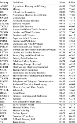
Table 1: Summary statistics of industry portfolios and explanatory variables.
Industry Definition Mean St.Dev.
AGRIC Agriculture, Forestry, and Fishing 0.499 7.987
MINES Mining 0.670 7.461
OIL Oil and Gas Extraction 0.809 7.095
STONE Nonmetalic Minerals Except Fuels 0.828 7.480
CNSTR Construction 0.672 7.114
FOOD Food and Kindred Products 0.678 4.149
SMOKE Tobacco Products 0.919 5.746
TXTLS Textile Mill Products 0.608 6.807
APPRL Apparel and Other Textile Products 0.509 6.624
WOOD Lumber and Wood Products 0.721 7.561
CHAIR Furniture and Fixtures 0.581 6.415
PAPER Paper and Allied Products 0.694 5.541
PRINT Printing and Publishing 0.545 5.562
CHEMS Chemicals and Allied Products 0.656 4.475 PTRLM Petroleum and Coal Products 0.824 5.047 RUBBR Rubber and Miscellaneous Plastics Products 0.736 5.983 LETHR Leather and Leather Products 0.759 6.734 GLASS Stone, Clay, and Glass Products 0.643 6.542 METAL Primary Metal Industries 0.502 7.002 MTLPR Fabricated Metal Products 0.674 5.164 MACHN Machinery, Except Electrical 0.708 6.153 ELCTR Electrical and Electronic Equipment 0.653 6.597
CARS Transportation Equipment 0.663 5.579
INSTR Instruments and Related Products 0.670 5.257 MANUF Miscellaneous Manufacturing Industries 0.631 6.455
TRANS Transportation 0.568 5.685
PHONE Telephone and Telegraph Communication 0.453 4.448 TV Radio and Television Broadcasting 0.897 6.604 UTILS Electric, Gas, and Water Supply 0.541 3.847
WHLSL Wholesale 0.621 5.465
RTAIL Retail Stores 0.663 5.031
MONEY Finance, Insurance, and Real Estate 0.633 5.200
SRVC Services 0.674 6.334
REIT Real Estate Investment Trust 0.480 5.170
RE Excess Market Return 0.581 4.319
MDY Market Dividend Yield 0.289 0.118
MVOL Market Volatility 4.016 2.193
DSPR Default Spread 0.073 0.033
CPI Consumer Price Index 0.317 0.457
3MTH 3-Month Treasury Bill 0.350 0.241
TS Term Spread 0.130 0.108
The table displays means and standard deviations of the variables used in the study. For the 34 industry portfolios, the variables are excess returns in excess of the one-month T-bill rate ranging from January 1946 to December 2012. The summary statistics for portfolio AGRIC are from July
1965 onwards and for portfolio REIT from January 1972 onwards. All variables are in monthly percentage points and at monthly frequency.
Table 2: In-sample predictive regressions between the metal industry portfolio and the market portfolio.
1946-2012 1946-2012 1946-2002 1946-2002 1946-1985 1946-1985
CONS T -0.408 -0.662 -0.972 -0.837 -1.849** -1.381** (0.609) (0.461) (0.632) (0.548) (0.712) (0.631)
MET ALt−1 -0.077* -0.073 -0.104** -0.106** -0.120** -0.118**
(0.046) (0.047) (0.040) (0.040) (0.055) (0.055)
REt−1 0.159** 0.143** 0.151** 0.133* 0.178** 0.138
(0.068) (0.069) (0.070) (0.072) (0.090) (0.090)
INFt−1 -0.977*** -0.871** -1.372*** -1.213*** -1.273*** -1.049***
(0.346) (0.339) (0.305) (0.305) (0.316) (0.325)
DS PRt−1 4.666 6.784 6.541
(6.707) (6.307) (6.659)
MDYt−1 3.487*** 4.031*** 4.504*** 4.897*** 5.680*** 5.671***
(1.146) (1.190) (1.381) (1.434) (1.617) (1.620)
MVOLt−1 -0.028 0.022 0.102
(0.091) (0.101) (0.115)
3MT Ht−1 -0.902*** -1.061*** -0.969***
(0.377) (0.380) (0.395)
T St−1 2.296 2.293 3.552*
(1.450) (1.604) (1.860)
R2 0.032 0.043 0.046 0.059 0.062 0.079
ad j.R2 0.025 0.035 0.038 0.051 0.050 0.067
T 804 804 684 684 480 480
The table presents in-sample results for predictive regressions (1) using three sample periods and two alternative specifications. The table illustrates the in-sample predictive power of industry portfolio METAL and additional explanatory variables. Robust standard errors are in
brackets. Notation *** corresponds with statistical significance at the 1% level,** at the 5% level, and * at the 10% level.
Table 3: In-sample static probit models with the metal industry portfolio.
1946-2012 1946-2012 1946-2002 1946-2002 1946-1985 1946-1985
CONS T 0.164 0.088 0.001 0.017 -0.291 -0.162
(0.180) (0.145) (0.210) (0.163) (0.038) (0.231)
MET ALt−1 -0.022** -0.022* -0.025* -0.025* -0.025 -0.025
(0.011) (0.011) (0.013) (0.013) (0.018) (0.018)
REt−1 0.044** 0.040** 0.038** 0.031* 0.051** 0.042*
(0.017) (0.017) (0.019) (0.019) (0.026) (0.024)
INFt−1 -0.433*** -0.406*** -0.495*** -0.457*** -0.474*** -0.431***
(0.110) (0.109) (0.121) (0.121) (0.128) (0.127)
DS PRt−1 0.160 -0.226 -0.042
(1.772) (2.056) (2.180)
MDYt−1 0.637 0.725* 1.017** 0.992** 1.414** 1.412**
(0.402) (0.413) (0.466) (0.470) (0.642) (0.644)
MVOLt−1 0.0004 0.020 0.039
(0.022) (0.026) (0.038)
3MT Ht−1 -0.190** -0.227** -0.223**
(0.094) (0.097) (0.110)
T St−1 0.447 0.411 0.069
(0.442) (0.493) (0.670)
psR2 0.033 0.038 0.032 0.037 0.031 0.034
ad j.psR2 0.027 0.032 0.024 0.030 0.021 0.023
log−L -529.323 -527.204 -450.294 -448.198 -314.392 -313.318
BIC 552.732 550.613 473.137 471.041 335.993 334.919
S R 0.619 0.624 0.611 0.624 0.612 0.612
DA 4.307*** 4.747*** 3.662*** 4.674*** 3.749*** 3.764***
PT 12.513*** 14.080*** 7.458*** 13.573*** 5.796** 6.743***
The table presents in-sample results for static probit models (6) including industry portfolio METAL as a explanatory variable. We use three sample periods and two alternative specifications. Robust standard errors in brackets, *** corresponds with significance at the 1% level,** at the
[image:15.595.78.523.424.736.2]Table 4: In-sample results for dynamic probit models with the METAL industry portfolio 1946M1-2012M12.
STATIC DYNAMIC AUTOREG. DYNAMIC AR.
CONS T 0.088 0.056 0.045 0.037
(0.145) (0.170) (0.086) (0.105)
MET ALt−1 -0.022* -0.022* -0.009 -0.009
(0.011) (0.011) (0.011) (0.011)
REt−1 0.040** 0.035* 0.018 0.017
(0.017) (0.021) (0.017) (0.019)
INFt−1 -0.406*** -0.403*** -0.206 -0.207
(0.109) (0.108) (0.218) (0.226)
MDYt−1 0.725* 0.730* 0.290 0.294
(0.413) (0.411) (0.314) (0.330) 3MT Ht−1 -0.190** -0.191** -0.108 -0.121
(0.094) (0.094) (0.129) (0.141)
T St−1 0.447 0.449 0.058 0.060
(0.442) (0.440) (0.157) (0.162)
yt−1 0.055 0.014
(0.154) (0.121)
πt−1 0.684* 0.681
(0.402) (0.421)
ad j.psR2 0.032 0.031 0.036 0.035
log−L -527.20 -527.13 -525.31 -525.30
BIC 550.61 553.89 552.06 555.40
S R 0.624 0.628 0.629 0.628
DA 4.747*** 5.062*** 5.164*** 5.062***
PT 14.080*** 17.179*** 19.680*** 15.248***
The table reports in-sample results for binary response models used in the study, including the METAL industry portfolio as a predictive variable. The sample period is 1946M1-2012M12. Results for subsamples and alternative specifications are available upon request. Robust standard errors
in brackets, *** corresponds with significance at the 1% level,** at the 5% level, and * at the 10% level.
Table 5: The industry portfolios and their in-sample predictive power.
INDUSTRY LEVEL STATIC DYNAMIC AUTOREG. DYNAMIC AR.
IND(−1) ad j.R2 IND(−1) ad j.psR2 IND(−1) ad j.psR2 IND(−1) ad j.psR2 IND(−1) ad j.psR2
MINES -0.035 0.033 -0.008 0.029 -0.008 0.028 -0.001 0.034 -0.001 0.033
(0.031) (0.007) (0.007) (0.006) (0.006)
OIL -0.037 0.032 -0.012 0.030 -0.012 0.029 -0.007 0.036 -0.007 0.035
(0.031) (0.008) (0.008) (0.007) (0.007)
STONE -0.053** 0.036 -0.003 0.028 -0.003 0.026 0.001 0.034 0.001 0.032
(0.024) (0.007) (0.007) (0.006) (0.008)
CNSTR -0.049 0.033 -0.018* 0.031 -0.018* 0.030 -0.005 0.035 -0.008 0.033
(0.032) (0.011) (0.011) (0.011) (0.076)
FOOD -0.028 0.031 -0.023 0.030 -0.023 0.029 -0.011 0.035 -0.011 0.034
(0.056) (0.015) (0.015) (0.019) (0.019)
SMOKE -0.047 0.033 -0.007 0.028 -0.006 0.027 -0.005 0.035 -0.006 0.033
(0.029) (0.008) (0.008) (0.008) (0.010)
TXTLS 0.008 0.030 -0.0008 0.027 3e-06 0.026 -0.004 0.034 -0.004 0.033
(0.030) (0.008) (0.008) (0.007) (0.007)
APPRL 0.027 0.031 0.004 0.027 0.004 0.026 0.002 0.034 0.002 0.033
(0.037) (0.011) (0.010) (0.012) (0.012)
WOOD -0.015 0.031 0.001 0.027 0.001 0.026 0.006 0.035 0.006 0.034
(0.028) (0.009) (0.009) (0.006) (0.006)
CHAIR -0.005 0.030 -0.003 0.027 -0.003 0.026 -0.004 0.034 -0.004 0.033
(0.039) (0.011) (0.011) (0.008) (0.008)
PAPER -0.034 0.031 0.003 0.027 0.003 0.026 -0.007 0.035 -0.006 0.033
(0.049) (0.013) (0.013) (0.010) (0.049)
PRINT 0.091* 0.035 0.022* 0.030 0.022* 0.029 0.019 0.037 0.020 0.035
(0.047) (0.013) (0.013) (0.017) (0.016)
CHEMS -0.006 0.030 0.006 0.027 0.006 0.026 0.010 0.035 0.010 0.034
(0.065) (0.019) (0.019) (0.016) (0.016)
PTRLM -0.090** 0.037 -0.017 0.030 -0.017 0.029 -0.006 0.034 -0.009 0.033
(0.040) (0.011) (0.011) (0.031) (0.064)
RUBBR -0.019 0.031 0.001 0.027 0.001 0.026 -0.011 0.036 -0.011 0.035
(0.041) (0.013) (0.013) (0.007) (0.007)
LETHR 0.021 0.031 -0.008 0.028 -0.008 0.027 -0.002 0.034 -0.002 0.033
(0.030) (0.008) (0.008) (0.007) (0.007)
GLASS -0.007 0.030 -0.006 0.028 -0.006 0.027 -0.012 0.037 -0.012 0.035
(0.038) (0.011) (0.011) (0.007) (0.008)
METAL -0.073 0.035 -0.022* 0.032 -0.022* 0.031 -0.009 0.036 -0.011 0.034
(0.047) (0.011) (0.011) (0.011) (0.103)
MTLPR -0.002 0.030 -0.016 0.028 -0.015 0.027 -0.013 0.036 -0.013 0.034
(0.059) (0.016) (0.016) (0.011) (0.010)
MACHN 0.045 0.031 0.014 0.029 0.014 0.027 0.007 0.035 0.007 0.033
(0.048) (0.013) (0.013) (0.013) (0.013)
ELCTR 0.018 0.031 0.003 0.027 0.003 0.026 -0.008 0.035 -0.008 0.034
(0.046) (0.013) (0.012) (0.008) (0.008)
CARS -0.057 0.032 -0.017 0.029 -0.017 0.028 -0.023*** 0.041 -0.023*** 0.040
(0.054) (0.014) (0.014) (0.008) (0.008)
INSTR 0.045 0.031 0.035** 0.033 0.035** 0.032 0.033 0.035 0.024 0.034
(0.052) (0.016) (0.016) (0.050) (0.014)
MANUF -0.009 0.030 -0.009 0.028 -0.009 0.027 -0.004 0.034 -0.004 0.033
(0.034) (0.009) (0.009) (0.007) (0.007)
TRANS -0.034 0.030 -0.002 0.027 -0.002 0.026 -0.010 0.036 -0.010 0.034
(0.043) (0.013) (0.013) (0.009) (0.009)
PHONE -0.003 0.030 0.011 0.028 0.011 0.027 0.013 0.037 0.013 0.036
(0.045) (0.012) (0.012) (0.009) (0.009)
TV 0.058* 0.034 0.021** 0.032 0.020** 0.031 0.011 0.036 0.013 0.035
(0.031) (0.010) (0.010) (0.035) (0.032)
UTILS 0.024 0.031 -0.010 0.028 -0.010 0.027 0.004 0.034 0.004 0.033
(0.061) (0.014) (0.014) (0.011) (0.011)
WHLSL 0.0002 0.030 -0.002 0.027 -0.002 0.026 -0.007 0.035 -0.007 0.033
(0.050) (0.015) (0.015) (0.010) (0.010)
RTAIL 0.061 0.032 0.0002 0.027 -0.0005 0.026 -0.008 0.035 -0.008 0.033
(0.059) (0.016) (0.016) (0.011) (0.011)
MONEY 0.131** 0.036 0.029* 0.030 0.029* 0.029 0.013 0.035 0.017 0.034
(0.066) (0.017) (0.017) (0.031) (0.048)
SRVC 0.061 0.032 0.009 0.028 0.008 0.027 0.008 0.035 0.008 0.034
(0.049) (0.014) (0.014) (0.008) (0.008)
AGRIC 0.068 0.018 0.005 0.018 0.006 0.016 0.007 0.018 0.006 0.016
(0.059) (0.013) (0.013) (0.029) (0.014)
REIT 0.017 0.016 0.003 0.018 0.003 0.016 0.001 0.017 0.001 0.015
(0.038) (0.010) (0.010) (0.011) (0.010)
NOIND 0.028 0.029 0.027 0.035 0.034
The results are obtained from models including lagged returns for one industry portfolio,REt−1,INFt−1,MDYt−1, 3MT Ht−1, andT St−1as explanatory variables for
Table 6: Out-of-sample results from predictive regressions and probit models with the METAL portfolio.
MODEL SR DA PT RETURN SHARPE LEVEL 0.586 1.546 1.549 9.65% 1.51 STATIC 0.642 2.887*** 7.576*** 12.30% 2.01 DYNAMIC 0.645 3.072*** 9.955*** 12.63% 2.08 AUTOREG. 0.617 1.869* 2.674 10.63% 1.63 DYNAMIC AR. 0.599 0.953 0.123 10.13% 1.53
[image:18.595.69.540.216.580.2]The table presents statistical and economic measures used to study the out-of-sample performance of the employed models. Statistical measures include the success ratio (SR) and both of the Pesaran and Timmermann (1992,2009) statistics (DA) and (PT). Economic measures include annual returns in percentages and ex-post Sharpe ratios (15) for trading strategies based on forecasting models including the METAL industry portfolios. The out-of-sample period is 1986M1-2012M12. The results from the predictive regressions (1) are denoted as "level". Notation *** corresponds with significance at the 1% level,** at the 5% level, and * at the 10% level.
Table 7: Out-of-sample results for predictive regressions and probit models
INDUSTRY LEVEL STATIC DYNAMIC AUTOREG. DYNAMIC AR.
SR PT SR PT SR PT SR PT SR PT
MINES 0.562 0.130 0.608 1.099 0.614 1.541 0.602 0.011 0.599 0.545
OIL 0.574 1.563 0.614 1.297 0.608 0.651 0.617 2.629 0.614 1.988
STONE 0.574 0.487 0.623 2.550 0.605 0.285 0.602 0.009 0.605 0.103
CNSTR 0.556 0.124 0.648 9.421*** 0.636 5.622** 0.614 0.985 0.602 0.110
FOOD 0.556 0.210 0.617 2.595 0.602 0.742 0.627 3.334* 0.605 0.002
SMOKE 0.580 2.947* 0.623 2.689 0.614 0.634 0.611 0.051 0.608 0.040
TXTLS 0.528 0.024 0.620 2.559 0.611 1.413 0.608 0.331 0.599 0.218
APPRL 0.571 1.965 0.611 0.968 0.605 0.504 0.571 0.386 0.580 0.527
WOOD 0.552 0.203 0.633 4.620** 0.611 0.757 0.580 0.241 0.571 0.351
CHAIR 0.549 0.121 0.620 1.487 0.620 2.324 0.611 0.001 0.602 0.019
PAPER 0.571 0.520 0.620 2.939* 0.605 0.991 0.602 1.535 0.611 0.078
PRINT 0.556 0.032 0.608 1.245 0.605 1.059 0.602 0.182 0.602 0.018
CHEMS 0.562 0.480 0.630 3.432* 0.614 0.751 0.617 1.132 0.611 0.096
PTRLM 0.549 0.013 0.623 3.682* 0.602 0.824 0.608 0.493 0.623 1.327
RUBBR 0.568 0.678 0.620 1.728 0.614 1.442 0.596 0.871 0.611 1.257
LETHR 0.552 0.005 0.614 1.400 0.614 1.531 0.586 0.259 0.586 0.228
GLASS 0.531 0.278 0.627 3.540* 0.620 2.325 0.590 0.020 0.602 0.001
METAL 0.586 1.548 0.642 7.576*** 0.645 9.955*** 0.617 2.674 0.599 0.124
MTLPR 0.571 1.171 0.627 2.796* 0.611 1.081 0.593 0.560 0.599 0.121
MACHN 0.580 1.387 0.586 0.237 0.586 0.104 0.602 0.594 0.586 0.037
ELCTR 0.559 0.003 0.611 0.867 0.608 0.542 0.574 0.438 0.583 0.198
CARS 0.565 0.212 0.627 3.157* 0.623 2.559 0.590 0.099 0.586 0.055
INSTR 0.559 0.004 0.608 2.007 0.593 0.535 0.586 0.192 0.611 0.022
MANUF 0.565 0.069 0.630 3.061* 0.617 1.302 0.590 0.330 0.596 0.015
TRANS 0.565 0.480 0.617 1.381 0.605 0.524 0.602 0.862 0.599 0.159
PHONE 0.562 0.001 0.605 0.222 0.599 0.006 0.593 0.244 0.617 1.073
TV 0.571 0.940 0.605 0.094 0.593 0.001 0.620 0.968 0.605 0.060
UTILS 0.556 0.205 0.605 0.744 0.605 0.843 0.605 0.038 0.605 0.003
WHLSL 0.549 0.001 0.623 2.542 0.602 0.179 0.620 0.613 0.602 0.001
RTAIL 0.565 0.405 0.617 1.816 0.605 0.502 0.602 0.070 0.605 0.004
MONEY 0.565 0.605 0.620 3.066* 0.620 2.682 0.605 0.058 0.602 0.292
SRVC 0.559 0.141 0.620 2.225 0.617 2.145 0.623 2.380 0.608 0.032
AGRIC 0.478 0.358 0.593 1.400 0.574 0.130 0.605 1.620 0.623 1.023
REIT 0.469 0.236 0.586 0.381 0.577 0.114 0.580 1.147 0.626 2.887*
NOIND 0.568 0.510 0.623 2.047 0.608 0.350 0.599 0.474 0.590 0.010
The table reports out-of-sample results for different models including the 34 industry portfolios and also a case where no industries are included (NOIND). Each model includes alsoREt−1,INFt−1,MDYt−1, 3MT Ht−1, andT St−1as explanatory variables. The reported statistics are the
success ratio (12) that tells the percentage of correct forecasts, and the Pesaran and Timmermann (2009) test statistic (14). Notation *** corresponds with significance at the 1% level,** at the 5% level, and * at the 10% level.
Table 8: Annual returns and Sharpe ratios of investment strategies using selected models
INDUSTRY MEASURE LEVEL STATIC DYNAMIC AUTOREG. DYNAMIC AR. CNSTR RETURN 8.29% 12.73% 12.08% 9.86% 8.66%
SHARPE 1.17 2.12 1.98 1.44 1.08 WOOD RETURN 8.26% 12.08% 11.06% 8.89% 8.68%
SHARPE 1.15 1.94 1.68 1.25 1.12 PTRLM RETURN 7.50% 10.67% 11.06% 10.79% 10.14%
SHARPE 0.95 1.57 1.75 1.67 1.43 NOIND RETURN 9.16% 11.60% 10.59% 9.57% 9.28%
SHARPE 1.39 1.82 1.58 1.37 1.32
The table presents annual returns in percentages and ex-post Sharpe ratios (15) for trading strategies based different on forecasting models including selected industry portfolios. The trading period is 1986M1-2012M12.
[image:18.595.92.502.640.751.2]Table 9: The Industry Portfolios and their predictive ability.
INDUSTRY LEVEL STATIC DYNAMIC AUTOREG. DYNAMIC AR.
IND(−1) ad jR2 IND(−1) ad j.psR2 IND(−1) ad j.psR2 IND(−1) ad j.psR2 IND(−1) ad j.psR2
MINES -0.062 0.061 -0.015 0.022 -0.014 0.022 0.001 0.031 0.001 0.029
(0.048) (0.014) (0.014) (0.009) (0.009)
OIL -0.053 0.061 -0.021 0.024 -0.021* 0.023 -0.003 0.031 -0.003 0.029
(0.043) (0.013) (0.013) (0.010) (0.010)
STONE -0.024 0.059 -0.005 0.021 -0.005 0.021 0.002 0.031 0.002 0.029
(0.025) (0.009) (0.009) (0.006) (0.006)
CNSTR -0.052 0.061 -0.017 0.023 -0.019 0.023 0.003 0.032 0.004 0.030
(0.045) (0.015) (0.015) (0.007) (0.007)
FOOD 0.039 0.058 -0.026 0.022 -0.023 0.021 0.002 0.031 0.002 0.029
(0.095) (0.027) (0.027) (0.015) (0.015)
SMOKE 0.003 0.058 0.005 0.021 0.005 0.021 0.003 0.031 0.003 0.029
(0.057) (0.017) (0.017) (0.009) (0.009)
TXTLS 0.054 0.060 0.016 0.022 0.015 0.021 0.007 0.032 0.007 0.030
(0.048) (0.017) (0.016) (0.011) (0.010)
APPRL 0.042 0.060 0.010 0.021 0.009 0.021 0.012 0.034 0.012 0.031
(0.039) (0.014) (0.014) (0.015) (0.017)
WOOD 0.046 0.060 0.008 0.021 0.008 0.021 0.014 0.036 0.014 0.034
(0.036) (0.013) (0.013) (0.009) (0.009)
CHAIR -0.022 0.058 -0.017 0.022 -0.017 0.022 -0.003 0.031 -0.003 0.029
(0.046) (0.016) (0.016) (0.010) (0.010)
PAPER 0.099 0.061 0.036 0.024 0.036 0.023 -0.011 0.032 -0.011 0.030
(0.083) (0.023) (0.023) (0.012) (0.011)
PRINT 0.133** 0.068 0.022 0.022 0.022 0.022 0.005 0.032 0.005 0.030
(0.059) (0.018) (0.018) (0.009) (0.008)
CHEMS -0.041 0.058 0.010 0.021 0.011 0.021 0.001 0.031 0.001 0.029
(0.101) (0.032) (0.032) (0.018) (0.017)
PTRLM -0.098* 0.065 -0.025 0.023 -0.024 0.023 0.002 0.031 0.002 0.029
(0.056) (0.016) (0.016) (0.009) (0.009)
RUBBR -0.012 0.058 -0.003 0.021 -0.003 0.020 -0.020** 0.036 -0.020** 0.034
(0.052) (0.018) (0.018) (0.010) (0.010)
LETHR 0.034 0.059 0.001 0.021 0.0003 0.020 0.011 0.033 0.011 0.031
(0.051) (0.016) (0.016) (0.009) (0.009)
GLASS -0.005 0.058 -0.015 0.021 -0.014 0.021 -0.003 0.031 -0.006 0.026
(0.065) (0.024) (0.024) (0.016) (0.019)
METAL -0.119** 0.067 -0.025 0.023 -0.026 0.023 -0.010 0.033 -0.010 0.031
(0.055) (0.018) (0.018) (0.010) (0.010)
MTLPR 0.062 0.059 -0.033 0.022 -0.034 0.022 -0.023 0.034 -0.023 0.032
(0.087) (0.028) (0.028) (0.016) (0.017)
MACHN 0.042 0.058 0.052** 0.026 0.052** 0.025 0.020 0.033 0.019 0.031
(0.094) (0.026) (0.026) (0.021) (0.022)
ELCTR 0.015 0.058 0.011 0.021 0.009 0.021 -0.023* 0.035 -0.022 0.033
(0.070) (0.026) (0.026) (0.012) (0.012)
CARS -0.025 0.058 -0.022 0.022 -0.023 0.022 -0.026 0.036 -0.026 0.034
(0.070) (0.021) (0.020) (0.018) (0.019)
INSTR 0.120** 0.066 0.060*** 0.033 0.058** 0.032 0.073*** 0.036 0.072*** 0.034
(0.052) (0.019) (0.019) (0.019) (0.018)
MANUF 0.030 0.059 0.006 0.021 0.006 0.021 0.008 0.033 0.009 0.032
(0.038) (0.013) (0.013) (0.057) (0.005)
TRANS 0.025 0.058 0.006 0.021 0.004 0.021 -0.009 0.032 -0.009 0.030
(0.054) (0.018) (0.018) (0.011) (0.010)
PHONE 0.063 0.060 0.030 0.023 0.030 0.023 0.010 0.032 0.010 0.030
(0.056) (0.019) (0.019) (0.041) (0.070)
TV 0.064** 0.063 0.020 0.024 0.019 0.023 0.007 0.032 0.007 0.030
(0.033) (0.012) (0.012) (0.007) (0.007)
UTILS -0.012 0.058 -0.035 0.023 -0.033 0.023 -0.007 0.031 -0.006 0.029
(0.084) (0.026) (0.025) (0.017) (0.017)
WHLSL 0.032 0.058 0.006 0.021 0.005 0.021 -0.001 0.031 -0.001 0.029
(0.059) (0.021) (0.021) (0.010) (0.010)
RTAIL 0.078 0.060 0.010 0.021 0.010 0.021 -0.001 0.031 -0.001 0.029
(0.069) (0.023) (0.023) (0.011) (0.011)
MONEY 0.214** 0.069 0.010 0.021 0.010 0.021 -0.002 0.031 -0.003 0.029
(0.090) (0.029) (0.028) (0.014) (0.014)
SRVC 0.087 0.063 0.013 0.022 0.013 0.021 0.009 0.033 0.009 0.031
(0.054) (0.017) (0.017) (0.006) (0.006)
These in-sample results are obtained from models including lagged returns for one industry portfolio,REt−1,INFt−1,MDYt−1, 3MT Ht−1, andT St−1as explanatory