Modified Adomain Decomposition Method for the
Generalized Fifth Order KdV Equations
Huda O. Bakodah
Department of Mathematics, Science Faculty for Girls, King Abdulaziz University, Jeddah, KSA Email: [email protected], [email protected]
Received September 23, 2012; revised November 6, 2012; accepted November 28, 2012
ABSTRACT
New modified Adomian decomposition method is proposed for the solution of the generalized fifth-order Korteweg-de Vries (GFKdV) equation. The numerical solutions are compared with the standard Adomian decomposition method and the exact solutions. The results are demonstrated which confirm the efficiency and applicability of the method.
Keywords: Modified Adomian Decomposition Method; Fifth Order KdV Equation; Solitary-Wave Solution
1. Introduction
The fifth-order (or generalized) KdV is the essential a model foe several physical phenomena including shal- low-water waves near critical value of surface tension and waves in nonlinear LC circuit with mutual induc- tance between neighbouring inductors [1]. Although no general solution is known, the exact solution of the fifth order KdV equation has been found for the special case of solitary waves in [2]. In general, the fifth order KdV need to be solved numerically. Commonly used numeri- cal methods to approximate the solutions of (gfKdV) include finite difference methods, collection methods and Galerkin methods. Kawahara [3] investigated the steady solutions of this equation on the basis of numerical cal- culations. Boyd [4] and Haupt and Boyd [5] reduced this equation to an ordinary differential equation and then a variety of analyticl and numerical methods are developed. The numerical methodes are based on Newton-Kan- torovich pseudo-spectral method and Newton-Kan- torovich Galerkin method. In [6] K. Djidjeli et al. pro- posed finite deference schemes based on a predictor - corrector algorithm and a linearized implicit method for the third and fifth order KdV equations.
However, some of these methods are not easy to use and sometimes require tedious work and calculation [7, 8]. In recent years, Adomian decomposition methods (ADM) [9] have emerged as a powerful tool for a wide class of nonlinear equation [10]. G. Adomian in [11] ap- plied his method to the 5th order KdV equation. In [12, 13], D. Kaya calculated the explicit and numerical solu- tions of some fifth-order KdV equation by decomposi- tion method and Kaya and El-Sayed in [14] proved the convergence of (ADM) applied to (gfKdV) equation.
A comparative study between (ADM) and Crank Nicholas method presented in [15]. (ADM) has led to several modifications on the method made by various researches in order to improve the accuracy or expansion of the application of the original method. Wazwaz [16] presented a reliable modification of the Adomian de- composition method.
In 2001, Wazwaz presented another type of modifica- tion [17] to the (ADM). Wazwaz modifications arises in the initial definition of the operator when applying the (ADM) to the nonlinear equation.
To the best of our knowledge, no attempt is made re- garding the solution of generalized fifth order KdV equa- tions by using modified decomposition method. So our main aim in this paper is used the modification ADM to solve the five particular class of the (gfKdV) equations. We generalized an appropriate Adomian’s polynomials for (gfKdV) equation will be handle more easily, quickly, and elegantly by implementing the new modified (ADM) rather than traditional methods for the exact solution of which is to be obtained subject to initial condition.
2. Fifth-Order KdV Equations
The well-known fifth-order KdV (fKdV) equations can be shown in the form
2
0
t x x xx xxx xxxxx
u au u bu u cuu du (1) where a, b, c and d are nonzeros and real parameters, and
,uu x t is a sufficiently smooth function. The (fKdV) is an important mathematical model with wide applica- tions in quantum mechanics and nonlinear optics.
quantum field theory. A variety of the (fKdV) equations can be developed by changing the real values of the pa- rameters a, b and c [18]. the derivation of these fifth- order forms are derived specific bilinear forms of the so-called Hirota’s D-operators. However, five will known forms of the (fKdV) that are of particular interest in the literature. These forms are:
1) The Sawada-Kotera (SK) equation is given by [19]
2
45 15 15 0
t x x xx xxx xxxxx
u u u u u uu u
0
(2) 2) The Caudrey-Dodd-Gibbon (CDG) equation is given by [20]
2
180 30 30 0
t x x xx xxx xxxxx
u u u u u uu u (3) 3) The Lax equations [21]
2
30 30 10 0
t x x xx xxx xxxxx
u u u u u uu u (4) 4) The Kaup-Kuperschmidt (KK) equation [22,23]
2
20 25 10 0
t x x xx xxx xxxxx
u u u u u uu u (5) 5) The Ito equation [24]
2
2 6 3
t x x xx xxx xxxxx
u u u u u uu u (6)
3. The Method of Soultion
3.1. Adomian Decomposition Method
In this section, we give outline and implement Adomian decomposition method for nonlinear equations to obtain analytic and approximate solutions which are obtained in a rapidly convergent series with elegantly computable components by this method. The Adomian approxima- tion series converge quickly. In general, convergence re- gions of the series are small. Now we outline of the me- thod here in order to obtain the solutions using (ADM), consider the fifth-order KdV Equation (1) in an operator form
0,t u u u x
L u aK bM cN dL u (7) where the notations 2 ,
u x
K u u Muu ux xx, and .
u xx
N uu x By symbolizing the nonlinear term, respec- tively. The notation Lt
t
and
5 5 x L x
symbolize
the linear differential operators. Assuming the inverse of operator exists and it can conveniently be taken as the definite integral with respect to from 0 to , i.e.,
1 t L t t
1 0 d t tL
t
(8)Thus, applying the inverse operator Lt1 to (7) yields;
1 1 1
1 1 0,
t t t u t u
t u t x
L L u aL K bL M cL N dL L u
(9)
Therefore, it follows that
1 1 1 1
, , 0
,
t u t u t u t x
u x t u x
aL K bL M cL N dL L u
(10)
Since initial value is known and we decompose the unknown function u x t
, as a sum of components de- fined by the decomposition series
0
, n
n
u x t u x t
, , (11)with u0 identified as u x
, 0 ,.
The nonlinear terms Ku Mu and u can be de-
composed into infinite series of polynomial given by
N 2 0 , u x n n
K u u A
(12)0
,
u x xx n
n
M u u B
(13)0
,
u xxxx n
n
N uu C
(14),
n
A and are the so-called Adomian poly- nomials of defined by
,
n
B Cn
, 0, 1, n.
u u u
=1 0
1 d
, 0,1, 2, . (15) ! d
n
k
n n k
k
P u n
n
nSubstituting (11-14) into (10) gives rise to
1 1 1 1
1 ,
1.
n t n t n t n t x
u aL A bL B cL C dL L u
n
(16)
The solution u x t
, must satisfy the requirements imposed by the initial conditions. Based on the (ADM), we constructed the solution u x t
, as
0 , , lim
where , , , 0.
n n
n
n k
k
u x t
x t u x t n
(17)The decomposition method provides a reliable techni- que that requires less work if we compared with the traditional techniques.
3.2. New Modified Adomian Decomposition Method
In the new modification by Wazwaz [17], we can replace the process of identified u0 as u x
, 0
by dividing
, 0u x by a series of infinite components. We therefore suggest that
0 0 0 , n nu x t u x
. (18)A new recursive relationship expressed in the form
0 0 0
1 1 1 1 1
1 0 ,
1.
n
n t n t n t n t
u u aL A bL B cL C dL L u
n
x n (19)
We can observe that algorithm (19) reduces the num- ber of terms involved in each component, and hence the size of calculations is minimized compared to the stan- dard (ADM) only. Moreover this reduction of terms in each component facilitates the construction of Adomian polynomials for nonlinear operators. the new modifi- cation overcomes the difficulty of decomposing u x
, 0 and introduces an efficient algorithm that improves the performance of the standard (ADM).4. Numerical Experiments
In this section, we consider some (gfKdV) equations for numerical comparisons based on the new modifications of (ADM). In this paper, we illustrate how the appro- ximate solutions of the (gfKdV) equations are close to exact solutions.
4.1. Example (1): (Sawada-Kotera Equation)
we consider the (S-K) Equation [25], with initial condi- tion is given by
2 2
0 , 2 sech 0 .
u x t k k xx
(20)
and the exact solution
2 2
4
0
, 2 sech 16 .
u x t k k x k t x (21)
Table 1 shows the difference of the analytical solution and numerical solution of the absolute errors only for 5 iterative.
4.2. Example (2): (Caudrcy-Dodd-Gbbon (C-D-G) Equation)
we consider the (C-D-G) equation, with initial condition
2
2 e
, 0 .
1 e
kx kx
k
u x
(22)
and the exact solution
4 4 2 2 e , 1 ek x k t
k x k t
k u x t
[image:3.595.310.540.264.377.2]. (23)
Table 2 shows the numerical results for example (2)
for k0.01.
4.3. Example (3): (The Lax Equation)
we consider Lax’s fifth order KdV equation with the
initial condition:
2
2
0
, 0 2 2 3 tanh .
u x k k xx (24)
and the exact solution
2
2
4
0
, 2 2 3 tanh 56
u x t k k x k tx . (25)
Table 3 shows the numerical results for example (3)
for k0.01, x00.0.
4.4. Example (4): (Kaup-Kuperschmidt (K-K) Equation)
We consider the (K-K) equation with the initial condition
2 2 22
24 e 4e e 16
, 0 .
16e e 16
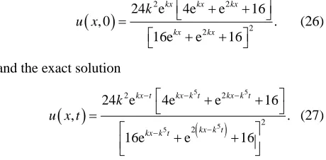
kx kx kx kx kx k u x (26)
and the exact solution
5 5 5 5 2 2 2 224 e 4e e 16
, .
16e e 16
kx t kx k t kx k t kx k t kx k t
k u x t
(27)
Table 4 shows the numerical results for example (4)
for 0.01k .
4.5. Example (5): (Ito Equation)
we consider the Ito equation with the initial condition
2 2 2
, 0 20 30 tanch .
u x k k kx (28) and the exact solution
22 2 4
0
, 20
30 tanch 96 .
u x t k
k kx k x
(29)
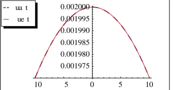
Table 5 shows the numerical results for example (5)
for k0.01 and x00.0.
5. Conclusions and Remarks
In this work, we proposed new modification of Adomian decomposition method. We solved the five well known forms of the (fKdV) equation with initial conditions. The method has been shown to computationally efficient in these examples that are important to researchers in ap- plied sciences. The obtained results in examples indicted that the new modification of (ADM) was feasible and effective. The method overcomes the difficulties arising in the modified decomposition method established in [16].
[image:3.595.57.286.551.678.2]Table 1. Absolute error between the exact solution and approximation solution for k = 0.01 and x0 = 0.0.
t/x 0.2 0.4 0.6 0.8 1.0 5.0
2 1.54499 × 10⁻¹⁸ 4.52654 × 10⁻¹⁸ 1.25496 × 10⁻¹⁷ 2.81893 × 10⁻¹⁷ 5.40204 × 10⁻¹⁷ 6.6435 × 10⁻¹⁵
4 5.36680 × 10⁻¹⁸ 1.12757 × 10⁻¹⁷ 2.7349 × 10⁻¹⁷ 5.87095 × 10⁻¹⁷ 1.10345 × 10⁻¹⁶ 1.32874 × 10⁻¹⁴
6 1.13841 × 10⁻¹⁷ 2.02746 × 10⁻¹⁷ 4.44252 × 10⁻¹⁷ 9.14253 × 10⁻¹⁷ 1.68892 × 10⁻¹⁶ 1.99336 × 10⁻¹⁴
8 1.97054 × 10⁻¹⁷ 3.15232 × 10⁻¹⁷ 6.37511 × 10⁻¹⁷ 1.26364 × 10⁻¹⁶ 2.29688 × 10⁻¹⁶ 2.6582 × 10⁻¹⁴
[image:4.595.57.540.240.346.2]10 3.02492 × 10⁻¹⁷ 4.50486 × 10⁻¹⁷ 8.52725 × 10⁻¹⁷ 1.63633 × 10⁻¹⁶ 2.92707 × 10⁻¹⁶ 3.32327 × 10⁻¹⁴
Table 2. Absolute error between the exact solution and approximation solution for k = 0.01 and x0 = 0.0.
t/x 0.2 0.4 0.6 0.8 1.0 5.0
2 1.96921 × 10⁻²¹ 3.11957 × 10⁻²¹ 3.63542 × 10⁻²¹ 1.7893 × 10⁻²⁰ 2.62474 × 10⁻²⁰ 2.48025 × 10⁻¹⁸
4 3.87141 × 10⁻²¹ 2.70138 × 10⁻²¹ 9.52285 × 10⁻²¹ 2.01336 × 10⁻²⁰ 5.33583 × 10⁻²⁰ 5.70681 × 10⁻¹⁸
6 7.39739 × 10⁻²¹ 5.50257 × 10⁻²¹ 2.20177 × 10⁻²⁰ 3.91461 × 10⁻²⁰ 7.69124 × 10⁻²⁰ 8.93996 × 10⁻¹⁸
8 1.89429 × 10⁻²¹ 4.74685 × 10⁻²¹ 2.75676 × 10⁻²⁰ 5.79897 × 10⁻²⁰ 9.69092 × 10⁻²⁰ 1.21797 × 10⁻¹⁷
[image:4.595.55.541.372.471.2]10 6.82819 × 10⁻²¹ 7.21049 × 10⁻²¹ 2.61724 × 10⁻²⁰ 5.63358 × 10⁻²⁰ 1.20126 × 10⁻¹⁹ 1.54092 × 10⁻¹⁷
Table 3. The exact and approximation solution of Lax equation for k = 0.01.
t/x 0.2 0.4 0.6 0.8 1.0 5.0
2 5.76197 × 10⁻¹⁴ 1.15211 × 10⁻¹³ 1.72788 × 10⁻¹³ 2.30342 × 10⁻¹³ 2.87867 × 10⁻¹³ 1.42104 × 10⁻¹² 4 1.15281 × 10⁻¹³ 2.30464 × 10⁻¹³ 3.45618 × 10⁻¹³ 4.60727 × 10⁻¹³ 5.75777 × 10⁻¹³ 2.84213 × 10⁻¹²
6 1.72985 × 10⁻¹³ 3.45759 × 10⁻¹³ 5.18489 × 10⁻¹³ 6.91153 × 10⁻¹³ 8.63729 × 10⁻¹³ 4.26326 × 10⁻¹²
8 2.3073 × 10⁻¹³ 4.61096 × 10⁻¹³ 6.91403 × 10⁻¹³ 9.21621 × 10⁻¹³ 1.15172 × 10⁻¹² 5.68444 × 10⁻¹²
10 2.88518 × 10⁻¹³ 5.76475 × 10⁻¹³ 8.64358 × 10⁻¹³ 1.15213 × 10⁻¹² 1.43976 × 10⁻¹² 7.10566 × 10⁻¹²
Table 4. Absolute error between the exact solution and approximation solution for k = 0.01 and x0 = 0.0.
t/x 0.2 0.4 0.6 0.8 1.0 5.0
2 1.46896 × 10⁻¹⁶ 7.86155 × 10⁻¹⁷ 1.0355 × 10⁻¹⁷ 5.77728 × 10⁻¹⁷ 1.25763 × 10⁻¹⁶ 2.24215 × 10⁻¹⁵
4 2.9378 × 10⁻¹⁶ 1.57193 × 10⁻¹⁶ 2.07239 × 10⁻¹⁷ 1.15638 × 10⁻¹⁶ 2.51752 × 10⁻¹⁶ 7.63093 × 10⁻¹⁶
6 4.40678 × 10⁻¹⁶ 2.35791 × 10⁻¹⁶ 3.10725 × 10⁻¹⁷ 1.73475 × 10⁻¹⁶ 3.77733 × 10⁻¹⁶ 7.15916 × 10⁻¹⁶
8 5.87582 × 10⁻¹⁶ 3.14383 × 10⁻¹⁶ 4.14144 × 10⁻¹⁷ 2.31306 × 10⁻¹⁶ 5.03728 × 10⁻¹⁶ 2.19495 × 10⁻¹⁵
10 7.34466 × 10⁻¹⁶ 3.92994 × 10⁻¹⁶ 5.17698 × 10⁻¹⁷ 2.89164 × 10⁻¹⁶ 6.29737 × 10⁻¹⁶ 3.67398 × 10⁻¹⁵
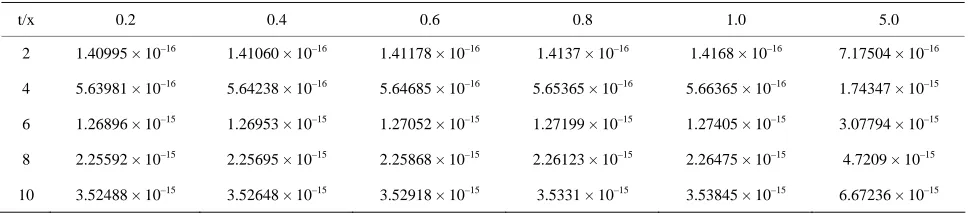
Table 5. Absolute error between the exact solution and approximation solution for k = 0.01 and x0 = 0.0.
t/x 0.2 0.4 0.6 0.8 1.0 5.0
2 1.40995 × 10⁻¹⁶ 1.41060 × 10⁻¹⁶ 1.41178 × 10⁻¹⁶ 1.4137 × 10⁻¹⁶ 1.4168 × 10⁻¹⁶ 7.17504 × 10⁻¹⁶
4 5.63981 × 10⁻¹⁶ 5.64238 × 10⁻¹⁶ 5.64685 × 10⁻¹⁶ 5.65365 × 10⁻¹⁶ 5.66365 × 10⁻¹⁶ 1.74347 × 10⁻¹⁵
6 1.26896 × 10⁻¹⁵ 1.26953 × 10⁻¹⁵ 1.27052 × 10⁻¹⁵ 1.27199 × 10⁻¹⁵ 1.27405 × 10⁻¹⁵ 3.07794 × 10⁻¹⁵
8 2.25592 × 10⁻¹⁵ 2.25695 × 10⁻¹⁵ 2.25868 × 10⁻¹⁵ 2.26123 × 10⁻¹⁵ 2.26475 × 10⁻¹⁵ 4.7209 × 10⁻¹⁵
[image:4.595.55.541.499.602.2] [image:4.595.56.540.628.735.2]10 5 0 5 10 0.0001985
0.0001990 0.0001995 0.0002000 ue
t
[image:5.595.80.264.85.187.2]
ua t
Figure 1. The ct and the approximation solution of s-k equation for t = 10 and k = 0.01.
exa
10 5 5 10
0.00002495 0.00002496 0.00002497 0.00002498 0.00002499 0.000025 ue
t
ua
t
Figure 2. The exact and the approximation solution of C-D-G equation for t = 10 and k = 0.01.
10 5 0 5 10
0.000395 0.000396 0.000397 0.000398 0.000399 0.000400 ue
t
[image:5.595.81.266.490.578.2]
ua t
Figure 3. The exact and the approximation solution of Lax equation for t = 10 and k = 0.01.
60 40 20 20 40 60 0.000042
0.000044 0.000046 0.000048 ue
t
[image:5.595.87.260.617.707.2]
ua
t
Figure 4. The exact and the approximation solution of K-K equation for t = 10 and k = 0.01.
10 5 0 5 10 0.001975
0.001980 0.001985 0.001990 0.001995 0.002000 ue
t
ua t
Figure 5. The exact and the approximation solution of Ito equation for t = 10 and k = 0.01.
tions of (gfKdV) equation with initial conditions and re- sults are found to be in good agreement with the exact solution as shown from Figures 1-5. In addition, no lin- earization or perturbation is required by the method.
REFERENCES
[1] H. Nagashima, “Experiment on Solitary Waves in the Nonlinear Transmission Line Discribed by the Equation
= 0 t
u uuu ,” Journal of the Physical Society of
Japan, Vol. 47, 1979, pp. 1387-1388. doi:10.1143/JPSJ.47.1387
[2] Y. Yamaoto and E. Takizawa, “On a Solution on Non-Linear Time—Evolution Equation of Fifth-Order,” Journal of the Physical Society of Japan, Vol. 50, 1981, pp. 1421-1422. doi:10.1143/JPSJ.50.1421
[3] T. Kawahrara, “Oscillatary Solitary Waves in Dispersive Media,” Journal of the Physical Society of Japan, Vol. 33, 1972, pp. 260-264. doi:10.1143/JPSJ.33.260
[4] J. P. Boyd, “Solitons from Sine Waves: Analytical and Numerical Methods for Non-Integrable Solitary and Con-oidal Waves,” Physica 21D, 1986, pp. 227-246.
[5] S. E. Haupt and J. P. Boyd, “Modelling Nonlinear Reso-nance: A Modification to the Stokes Perturbation Expan-sion,” Wave Motion, Vol. 10, No. 1, 1988, pp. 83-98. [6] K. Djidjeli, W. G. Price, E. H. Twizell and Y. Wang,
“Numerical Methods for the Soltution of the Third and Fifth-Order Disprsive Korteweg-De Vries Equations,” Journal of Computational and Applied Mathematics, Vol. 58, No. 3, 1995, pp. 307-336.
doi:10.1016/0377-0427(94)00005-L
[7] A. M. Wazwaz, “Analytic Study on the Generalized KdV Equation: New Solution and Periodic Solutions,” Elsevier, Amsterdam, 2006.
[8] M. T. Darvishi and F. Khani, “Numerical and Explicit Solutions of the Fifth Order Korteweg-De Vries Equa-tions,” Elsevier, Amsterdam, 2007.
[9] G. Adomian, “Solving Frontier Problems of Physics: The Decomposition Method,” Kluwer Academic Publisher, Dordrecht, 1994.
[10] D. Kaya, “The Use of Adomian Decomposition Methods for Solving a Specific Nonlinear Partial Differential Equations,” Bulletin of the Belgian Mathematical Society Simon Stevin, Vol. 9, No. 3, 2002, pp. 343-349.
[11] G. Adomian, “The Fifth-Order Korteweg-De Vries Equa-tion,” International Journal of Mathematics and Mathe-matical Sciences, Vol. 19, No. 2, 1996, p. 415.
doi:10.1155/S0161171296000592
[12] D. Kaya, “An Explicit and Numerical Solutions of Some Fifth-Order KdV Equation by Decomposition Method,” Applied Mathematics and Computation, Vol. 144, No. 2-3, 2003, pp. 353-363. doi:10.1016/S0096-3003(02)00412-5 [13] D. Kaya, “An Application for the Higher Order Modified
KdV Equation by Decomposition Method,” Communica-tions in Nonlinear Science and Numerical Simulation, Vol. 10, No. 6, 2005, pp. 693-702.
[14] D. Kaya and S. M. El-Sayed, “On a Generalized Fifth Order KdV Equations,” Physics Letters A, Vol. 310, No. 1, 2003, pp. 44-51. doi:10.1016/S0375-9601(03)00215-9 [15] M. A. Helal and M. S. Mehanna, “A Comparative Study
between Two Different Methods for Solving the General Korteweg-De Vries Equation (GKDV),” Chaos, Solitons & Fractals, Vol. 33, No. 3, 2007, pp. 725-739.
doi:10.1016/j.chaos.2006.11.011
[16] A. M. Wazwaz, “A Reliable Technique for Solving Lin-ear and NonlinLin-ear Schrodinger Equations by Adomian Decompostion Method,” Bulletin of the Institute of Mathematics, Vol. 29, No. 2, 2001, pp. 125-134.
[17] A. M. Wazwaz and S. M. El-Sayed, “A New Modifica-tion of the Adomian DecoomposiModifica-tion Method for Linear and Nonlinear Operators,” Applied Mathematics and Computations, Vol. 122, 2001, pp. 393-405.
[18] A. M. Wazwaz, “Partial Differential Equations and Soli-tary Waves Theory,” Higher Education Press, Beijing; Spinger-Verlag, Berlin, 2009.
[19] K. Sawada and T. Kotera, “A Method for Finding N-Soliton Solutions of the KdV. Equation and the KbV- Like Equation,” Progress of Theoretical Physics, Vol. 51, No. 5, 1974, pp. 1355-1367. doi:10.1143/PTP.51.1355
[20] P. J. Coudery, R. K. Dodd and J. D. Gibbon, “A New Hierarchy of Korteweg-De Vries Equations,” Proceed-ings of the Royal Society A, Vol. 351, No. 1666, 1976, pp. 407-422. doi:10.1098/rspa.1976.0149
[21] P. D. Lax, “Integrals of Nonlinear Equations of Evolution and Solitary Waves,” Communications on Pure and Ap-plied Mathematics, Vol. 21, No. 5, 1968, pp. 467-490. doi:10.1002/cpa.3160210503
[22] D. J. Kaup, “On the Iverse Scattering Problem for Cubic Eigenvalue Problems of the Class
6 6 =
xxx Q x R
,” Studies in Applied Mathe-matics, Vol. 62, 1980, pp. 189-216.
[23] B. A. Kuperschmidt, “A Super KdV Equation: An Inte-gral System,” Physics Letters A, Vol. 102, No. 5-6, 1984, pp. 213-215. doi:10.1016/0375-9601(84)90693-5
[24] M. Ito, “An Extension of Nonlinear Evolution Equations of the KdV (mKdV) Type of Higher Orders,” Journal of the Physical Society of Japan, Vol. 49, No. 2, 1980, pp. 771-778. doi:10.1143/JPSJ.49.771