The Approximated Semi Lagrangian WENO Methods Based on Flux Vector Splitting for Hyperbolic Conservation Laws

http://www.scirp.org/journal/ajcm ISSN Online: 2161-1211

ISSN Print: 2161-1203

The Approximated Semi-Lagrangian WENO

Methods Based on Flux Vector Splitting for

Hyperbolic Conservation Laws

Fuxing Hu

Department of Mathematics, Huizhou University, Huizhou, China

Abstract

The paper is devised to combine the approximated semi-Lagrange weighted essentially non-oscillatory scheme and flux vector splitting. The approximated finite volume semi-Lagrange that is weighted essentially non-oscillatory scheme with Roe flux had been proposed. The methods using Roe speed to construct the flux probably generates entropy-violating solutions. More se-riously, the methods maybe perform numerical instability in two-dimensional cases. A robust and simply remedy is to use a global flux splitting to substitute Roe flux. The combination is tested by several numerical examples. In addi-tion, the comparisons of computing time and resolution between the classical weighted essentially non-oscillatory scheme (WENOJS-LF) and the semi-La- grange weighted essentially non-oscillatory scheme (WENOEL-LF) which is presented (both combining with the flux vector splitting).

Keywords

Semi-Lagrangian Method, WENO Scheme, Flux Splitting

1. Introduction

The semi-Lagrangian methods are popularly used in weather prediction [1][2]

and simulation of the Vlasov equations [3][4][5][6], and so on. These methods solve the problems with a characteristic tracing algorithm. It is this property of algorithm that leads to the following two advantages: no time discretization and the alleviation of CFL time step restriction. The semi-Lagrangian methods

(combined wih WENO reconstruction [7] [8]) used to solve hyperbolic

problems are presented in [9][10][11].

In [10], the authors proposed a finite volume semi-Lagrangian WENO scheme

for advection problems. The scheme combined the Eulerian-Lagrangian How to cite this paper: Hu, F.X. (2017)

The Approximated Semi-Lagrangian WENO Methods Based on Flux Vector Splitting for

Hyperbolic Conservation Laws. American

Journal of Computational Mathematics, 7, 40-57.

https://doi.org/10.4236/ajcm.2017.71004

Received: February 23, 2017 Accepted: March 28, 2017 Published: March 31, 2017

Copyright © 2017 by author and Scientific Research Publishing Inc. This work is licensed under the Creative Commons Attribution International License (CC BY 4.0).

http://creativecommons.org/licenses/by/4.0/

framework [12][13] with high-order WENO reconstruction, and used a integral- based WENO reconstruction to handle trace-back integration. In this framework,

the scheme trace each computational Eulerian grid cell at time n1

t + backward

over a time step along the characteristic line to its Lagrangian track-back region

at n

t . The average mass is simply transported from the Lagrangian region to the

computational grid cell. In addition, they presented a theoretical proof for the accuracy of the method.

In [11], the authors developed a finite volume semi-Lagrangian WENO

scheme for nonlinear conservation laws. This method can be regarded as the

extension of the method for advection problems in [10]. A problem appeared in

such extension is that one does not have the particle velocity since it is nonlinearly related to the unknown solution. Hence, one cannot find the exact tracking line of fluid particle. Instead of trying to find the the exact characteristic line of particle, they use a known velocity for the tracing line computation. Since this will not give the correct tracing line, a flux correction procedure is needed to increase the accuracy and numerical stability. The proposed method arrives optimal order of accuracy. However, the procedure of flux correction makes the scheme rather cost to be implemented.

In [9], a sort of finite difference semi-Lagrangian ENO and WENO schemes

are devised for advection problems in incompressible flow. The key part of this paper is that the integral form of advection equation is taken over a triangle region. This integral procedure transforms the flux integration in time at cell center into the integration of mass u x t

( )

, n in space

(

)

(

)

( )

1

, d , d ,

n i

n i

t x _n

i

t f u x t t xu x t x

+

∗ =

∫

∫

where xi

∗ _{is backward characteristic point of cell center}

i

x . This scheme is

difficult to extent to nonlinear cases. In addition, there is no optimal linear weights for WENO schemes for solving advection equations with variable coefficients (or also for nonlinear cases).

In [14], the authors developed an approximated finite volume semi-Lagrangian

WENO schemes (WENOEL-Roe) for 1D and 2D nonlinear hyperbolic prolems. The scheme integrates the hyperbolic equation over the control volume

1

1 2, 1 2 ,

n n

i i

x− x+ t t + 

  ×

    to obtain a integral equation. They try to directly

evaluate the integration of flux function in time at cell edge xi+1 2.

(

)

(

)

1

1/ 2, d .

n n t

i

t f u x t t

+

+

∫

For linear cases, the integration of flux function in time can be transformed into the integration of interpolation polynomial of flux average in space. For nonlinear cases, a local freeze method is used to freeze the nonlinear into linear cases. The scheme here is different with the traditional semi-Lagrangian scheme

[10][11]. The backward tracing characteristic point is needed in the procedure

of evaluating the integration of flux function. The advantages of the WENOEL- Roe scheme are easy implement and high efficiency. Refer to [14] for a detail.

the direction of upwind. The Roe average speed is used to identified the upwinding. It is known that the Roe schemes maybe generates entropy-violating solutions. More seriously, these scheme can perform numerical instability for

some two-dimensional problems [15][16] [17]. A local entropy correction can

be used to remedy this deficiency. However, it is usually more robust to use a global flux splitting. In this paper, an approximated finite volume semi- Lagrangian WENO scheme with the smooth Lax-Friedrichs flux splitting (WENOEL-LF) is presented. The WENOEL-LF scheme is less resolution than WENOEL-Roe since the Lax-Friedrichs flux splitting method is more dissipative than Roe method. However, the advantage of WENOEL-LF scheme is it generally generates the entropy solution.

In the paper that follows, we will review the WENOEL-Roe scheme briefly in Section 2. In Section 3, we will present the formulation of WENOEL-LF scheme in Section 3 in detail. The comparisons of resolution and computing time between the WENOEL-LF and WENOJS-LF schemes is presented in Section 4.

2. Review the WENOEL-Roe Scheme

Consider the linear advection equation

( )

,

(

( )

,

)

0, , 0,

t x

u x t + f u x t = a≤ ≤x b t≥ (1)

where fx

(

u x t

( )

,

)

=au x t

( )

, . Integrating the Equation (1) on control volume

1

1 2, 1 2 ,

n n

i i

x₋ x₊ t t + 

  ×

    and rearranging this equation gives

(

)

(

)

(

(

)

)

(

)

(

)

1

1 2 1 2

1 2 1 2

1

1 1/ 2

1 2

1 1 1

, d , d , d

1

, d .

n i i n i i n n

x x t

n n i

x x t

t

i t

t

u x t x u x t x f u x t t

x x x t

f u x t t

t + + + − − + + − + ∆  = + _ ∆ ∆ ∆ ∆  − _ ∆ 

∫

∫

∫

∫

(2)

Denote the i-th cell average by

(

)

1 2 1 2 1

, d ,

i i

x n

i _x n

u u x t x

x + −

=

∆

∫

and average flux at cell edge xi+1 2 by

(

)

(

)

1

1 2 1/ 2

1

, d ,

n n

t n

i _t i

f f u x t t

t +

+ =_∆

∫

+ (3)

then (2) can be written as

(

)

1

1 2 1 2 .

n n n n

i i i i

t

u u f f

x

+

+ −

∆

= − −

∆ (4)

Denote the value n

i

U approximates the average value u_ij and the numerical

flux 1 2

n i

F+ approximates flux function 1 2

n i

f+ . Then we obtain

(

)

1

1 2 1 2 .

n n n n

i i i i

t

U U F F

x

+

+ −

∆

= − −

∆ (5)

For evaluating average flux 1 2

n i

f+ in (3), we can firstly apply a 5th-order

reconstruction based on piecewise constant average fluxes

{ }

1

N k k

f ₌ on stencil

{

2, 1, , 1, 2

}

i i i i i i

(

)

(

)

( )

( )

5

,n i .

f u x t =P x + ∆x (6)

Here, we assume the advection velocity a>0, then u x t

(

,n

)

simply spreads to the right with velocity a, which gives

(

)

(

i1/ 2,

)

(

(

i 1 2

(

n

)

, n

)

)

f u x+ t = f u x+ −a t−t t (7)

in any time when t∈

[

t tn, n+1

]

. Combining the formulas (6) with (7), the flow

rate f u x t

(

( )

,

)

at cell edge xi+1 2 is

(

)

(

)

(

(

)

)

( )

5

1 2, 1 2 .

i i i n

f u x+ t =P x+ −a t−t + ∆x (8)

In this case, the average flux 1 2

n i

f+ can be expressed approximately as

(

)

(

)

(

)

(

)

( )

( )

( )

1 1 1 2 1 2

1 2 1 2

5 1 2 5 1 , d 1 d 1 d . n n n n i i t n

i _t i

t

i i n

t

x i x a t

f f u x t t

t

P x a t t t x

t

P x x x

a t + + + + + + + − ∆ = ∆ = − − + ∆ ∆ = + ∆ ∆

∫

∫

∫

  (9)

Omitting the high-order term

( )

5

x

∆

 , we obtain the numerical flux

( )

1 2

1 2

1 2

1

= xi d .

n

i _{x a t} i

i

F P x x

a t

+ + _{− ∆}

+

∆

∫

(10)

The last equality in (9) is obtained by integration of substitution

(

)

1 2

i n

x=x₊ −a t−t . From the Equation (9), the integration in time

[

t t_n, _n+1

]

is

transformed into integration in space xi+1 2− ∆a t x, i+1 2. Due to the integrand

( )

i

P x is reconstruction polynomial, the last integration in (10) can be computed

exactly.

In the following of this section, we will present the 5th-order WENO reconstruction process to approximate the integral in (10)

( )

1 2 1 2 d . i i x i

x a tP x x

+ + − ∆

∫

The 5th-order WENO reconstruction procedure is represented as the convex combination of three 3rd-order reconstructions. First, we intend to reconstruct

three 3rd-order conservative polynomials j

( )

i

P x on cell Ii= xi−1 2,xi+1 2 based on the piecewise constant average fluxes on stencils

{

}

{

}

{

}

0 1 2

1 2 1 1 2 1

, , , , , , , , ,

i i i i i i i i i i i i

S = I I+ I+ S = I− I I+ S = I− I− I

where the subscript i denotes the polynomial on cell Ii and superscript j

denotes the reconstruction based on stencil j

i

S . So far, we have obtained the

conservative interpolation polynomials j

( )

i

P x on each stencil j

i

S . In the end, the integral in (10) can be expressed as

( )

( )

1 2 1 2

1 2 1 2

2

=0

d d ,

i i

i i

x _j x _j

i i

x a t x a t

j

P x x d P x x

+ +

+ − ∆ =

∑

+ − ∆

∫

∫

where j

d are the optimal weights. To alleviate the effect of the non-smooth

0 1 2

j

j i

i

i i i

a w

a a a

=

+ + (11)

and

(

)

2,

j j i j i d a ε β =

+ (12)

where j

i

β is the indicator of smoothness of the polynomial on the stencil j

i

S .

Finally, the numerical flux should be expressed as

( )

1 2 1 2 2 1 2 0 1 d . i i x

n j j

i i _{x a t} i

j

F w P x x

a t + + + _{− ∆} = =

∆

∑ ∫

(13)

Substituting the formula of polynomial j

( )

i

P x into (13) gives

( )

(

)

(

) (

)

(

)

(

)

(

) (

)

(

)

(

)

(

) (

)

(

)

1 2 1 2 2 1 2 0 0 2

1 2 1 1 2

1 2

1 1 1 1 1

2 2

2 1 2 1 2 1

1

d

1

2 3 3 2 5

6

2 3 3 5 2

2 3 9 6 2 7 11 .

i i x

n j j

i i _{x a t} i

j

i i i i i i i i i

i i i i i i i i i

i i i i i i i i i i

F w P x x

a t

w f f f f f f f f

w f f f f f f f f

w f f f f f f f f f

λ λ λ λ λ λ + + + _{− ∆} = + + + + + − + + − + − − − − − − = ∆  = _ − + + − + + − + − + + − + − + +  + − + + − + − + − + _

∑ ∫

(14)

In contrast, when the advection velocity a<0, u x t

(

, _n

)

spreads to the left

with velocity a, which gives

(

)

(

i1 2,

)

(

(

i 1/ 2

(

n

)

,n

)

)

f u x+ t = f u x+ −a t−t t (15)

and the flow rate f u x t

(

( )

,

)

at cell edge xi+1 2 is

(

)

(

)

(

(

)

)

( )

5

1 2, 1 1/ 2 .

i i i n

f u x+ t =P+ x+ −a t−t + ∆x (16)

Similarly, the average flux 1 2

n i

F+ can be expressed as

( )

1 2 1 2

2

1 2 1 1

0

1

d .

i i

x a t

n j j

i i _x i

j

F w P x x

a t + + − ∆ + + + = =

− ∆

∑ ∫

(17)

The nonlinear weight 1

j i

w₊ can be constructed similarly as (11) and (12).

Substituting the formula of polynomial 1

( )

j i

P+ x into (17) gives

(

) (

)

(

(

)

)

(

(

)

(

) (

)

)

(

) (

) (

)

(

)

0 2

1 2 1 1 2 3 1 2 3

1 2

1 2 3 1 1 2

1 1 2

2 2

1 1 1 1 1 1

1

2 6 9 3

6

11 7 2 2

3 3 2 5

2 3 3 5 2 .

n

i i i i i i i i

i i i i i i i

i i i i i

i i i i i i i i i

F w f f f f f f

f f f w f f f

f f f f f

w f f f f f f f f

λ λ λ λ λ λ + + + + + + + + + + + + + + + + + + − + + − +  = _ − + + − + + − + + − + + − + + −  + − + + − + − + + _ (18)

propagation direction is distinguished by Rankine-Hugoniot jump conditions

and propagation velocity is chosen to be

( )

i u u f u a u ₌ ∂ = ∂

(if propagation direction>0) or

( )

1 i u u f u a u + = ∂ = ∂

(if propagation direction<0).

3. Formulation of WENOEL-LF Scheme

In this section, we solve nonlinear problems by using a more robust global flux splitting

( )

( )

( )

f u = f+ u + f− u (19)

where

( )

( )

d d

0 and 0.

d d

f u f u

u u

+ −

≥ ≤

Insert the Equation (19) into (1) and (2), we can obtain

(

)

(

)

1 , , , ,

1 2 1 2 1 2 1 2 ,

n n n n n n

i i i i i i

t t

u u f f f f

x x

+ + + − −

+ − + −

∆ ∆

= − − − −

∆ ∆ (20)

which is similar to conservation formula (4), and denote

(

)

(

)

1

,

1 2 1 2

1

, d .

n n

t n

i _t i

f f u x t t

t +

± ±

+ = _∆

∫

+

A scheme approximated (20) can be written as

(

)

(

)

1 , , , ,

1 2 1 2 1 2 1 2 .

n n n n n n

i i i i i i

t t

U U F F F F

x x

+ + + − −

+ − + −

∆ ∆

= − − − −

∆ ∆ (21)

This scheme is conservative. Since if we sum n1

i

U + over the whole set of cells, we obtain

(

) (

)

(

)

1 , , , ,

1 2 1 2 1 2 1 2

1 1

.

N N

n n n n n n

i i N N

i i

t

U U F F F F

x + + − + − + + = = ∆ = − + − + ∆

∑

∑

The formulas , ,

1 2 1 2

n n

N N

F ₊+ +F ₊− and , ,

1 2 1 2

n n

F ++F − denote the fluxes at the

extreme edges. The sum of the flux differences cancels out except for the fluxes at the extreme.

The simplest smooth flux splitting we chose is the Lax-Friedrichs splitting

( )

1

(

( )

)

1

(

( )

)

, ( ) ,

2 2

f+ u = f u +αu f− u = f u −αu

where α _{is taken as}

( )

1 d max d i u N f u u α ≤ ≤

= _{over the whole set of cell averages. Since}

( )

d 0 d f u u +

≥ _{, the fluxes} f+

( )

u flow right through the cell edges. The flow

velocity a+ for flux f+

( )

u at cell edge xi+1 2 is chosen as

( )

d 1 2 d i u u f u a u α + + =     = +    

edge xi+1 2 is chosen as

( )

1 d 1 2 d i u u f u a u α + − − =     = −    .

Inserting f+

( )

u and f−

( )

u into (14) and (18), respectively, the numerical

fluxes can be obtained as follows,

( ) (

)

(

) (

)

(

)

( ) (

)

(

)

(

(

)

)

(

( ) (

)

(

) (

)

)

2 , 0

1 2 1 2 1 1 2

2 1

1 1 1

2 2

1 1 2 1

2 1 2 1

1

2 3 3 2 5

6

2 3 3

5 2 2

3 9 6 2 7 11 ,

n

i i i i i i i i i i

i i i i i i

i i i i i i i

i i i i i i

F w f f f f f f f f

w f f f f f

f f f w f f f

f f f f f f

λ λ λ λ λ λ + + + + + + + + + + + + + + + + + + + + + + + + − + + + + + + + + + − + − − + + + + + + + − − − −  = − + + − + + −  + − + + − + − + + + − +  + − + − + − + _ (22)

where a t

x

λ+ ₌ +∆

∆ , and

( ) (

)

(

)

(

(

)

)

(

( ) (

)

(

) (

)

)

( ) (

)

(

)

2 , 0

1 2 1 1 2 3 1 2 3

2 1

1 2 3 1 1 2

1 1 2

2 2

1 1 1 1 1

1

2 6 9 3

6

11 7 2 2

3 3 2 5

2 3 3 5 2

n

i i i i i i i i

i i i i i i i

i i i i i

i i i i i i i i i

F w f f f f f f

f f f w f f f

f f f f f

w f f f f f f f f

λ λ λ λ λ λ − − − − − − − − − + + + + + + + + − − − − − − − + + + + + + − − − − − − + + + − − − − − − − − − + − + + −  = − + + − +  + − + + − + + − + + −

+

(

− + + − + −

(

+ + −₁

)

)

+ _

(23)

where a t

x

λ− ₌ −∆ ∆ .

Algorithm

Here, we conclude the algorithm for computing the approximated solution n1

i

U +

at time step n1

t + .

1) Split the flux function f u

( )

into the positive flux f+

( )

u and negative

flux f−

( )

u .

2) Determine the flow velocities a+ and a− of the positive flux f+

( )

u

and negative flux f−

( )

u , respectively.

3) Compute the numerical fluxes ,

1 2

n i

F+± and 1 2,

n i

F−± by formulas (22) and

(23).

4) Insert the numerical fluxes computed above into (21), we obtain the

approximated solution n 1

i

U + at time step tn+1.

4. Numerical Results

4.1. Burgers’ Equation

Consider the inviscid Burgers’ equation 2

0 2 t

x

u u +_ _ =

  (24)

with two initial conditions:

( )

, 0 1 1 0,

0 0 1,

x u x

x

− ≤ ≤ 

=  _{≤ ≤}

 (25)

and

( )

, 0 1.5 sin

( )

π .

u x = − x (26)

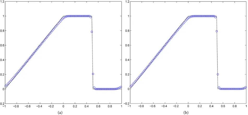
The Burger’s Equation (24) with discontinuous initial condition (25) develops the solution which consists of a rarefaction wave and a shock wave. The numerical solutions computed by the WENOEL-LF and WENOJS-LF schemes

are shown in Figure 1. These two solutions are both computed with N=100

and CFL = 0.1. The final output time is chosen to be t=1. From Figure 1, we

can find that the solution of WENOJS-LF scheme has slightly better resolution than that of WENOEL-LF scheme, especially around the rarefaction wave. And, in solving nonlinear cases (including the following tests), the WENOJS-LF scheme generally possesses slightly higher resolution than WENOEL-LF scheme when the same amount of cells is used.

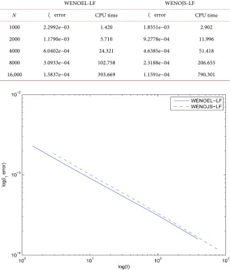
Although the WENOJS-LF scheme has higher resolution than WENOEL-LF scheme, the WENOEL-LF scheme has the advantage of decreasing the

computing time. Table 1 presents the l1 error and computing time. With the

same number of cells, the errors generated by WENOEL-LF are larger than WENOJS-LF scheme, but the computing times of WENOEL-LF are only half of

[image:8.595.62.538.481.701.2]

(a) (b)

that of the WENOJS-LF scheme. For comparing the efficiency between these two schemes, we plots the relationship between the l1 error and computing time for

these two schemes. From Figure 2, we can find that the efficiency of

WENOEL-LF is higher than that of WENOJS-LF scheme. That is, to achieve the

same l1 error, the WENOEL-LF needs less computing time.

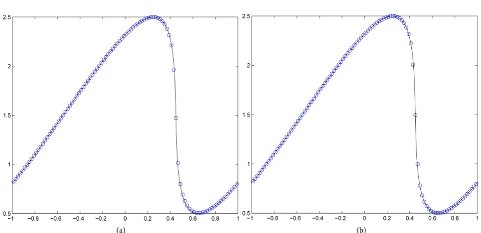
For the problem (24) (26), the initial condition is smooth, and the solution evolves discontinuity at t=1_π. The Figure 3 is plotted with N =100 and output

time t=0.3. From this figure, no obviously difference is presented (however, by

[image:9.595.208.539.317.705.2]

closed inspection, the resolution of WENOJS-LF is still slightly better than WENOEL-LF scheme). Similar to the last test, the superiority of our scheme lies in decreasing the computing time. Therefore, in efficiency, the WENOEL-LF scheme is still advantageous over the WENOJS-LF scheme.

Table 1. The comparisons of computing time (in seconds) and l1 error for initial value problem (24) (25) between the WENOEL-LF and WENOJS-LF methods.

WENOEL-LF WENOJS-LF

N l1 error CPU time l1 error CPU time

1000 2.2992e−03 1.420 1.8551e−03 2.902

2000 1.1790e−03 5.710 9.2778e−04 11.996

4000 6.0402e−04 24.321 4.6385e−04 51.418

8000 3.0933e−04 102.758 2.3188e−04 206.655

16,000 1.5837e−04 393.669 1.1591e−04 790.301

[image:10.595.56.539.58.292.2]

(a) (b)

Figure 3. The solutions of problem (24) (26) are computed by the WENOEL-LF and WENOJS-LF methods: (a) WENOEL-LF scheme; (b) WENOJS-LF scheme.

4.2. The 1D Euler Equation

In this subsection, we consider 1D Euler equations since one of the main application areas of high-resolution scheme is compressible gas dynamics,

(

)

2

0,

t x

u

u u p

E E p u

ρ ρ

ρ ρ

 

 

 

 _{ + + =}

 

 

   ₊ 

   

(27)

where ρ , u , p, E are density, velocity, pressure and total energy,

respectively. The system of equations is closed by the equation of state for an ideal polytropic gas:

2 1

,

1 2

p

E ρu

γ

= +

−

where the ratio of specific heats γ =1.4.

The following three initial conditions combined with Euler Equation (27) are considered, which are often used to examine the methods for solving Euler equations:

(

) (

₍

0.445, 0.698, 3.528 ,

₎

)

if 5 0, , ,

0.5, 0, 0.571 , if 0 5,

x u p

x

ρ =  − ≤ <_{≤ ≤}

 (28)

(

)

( )

(

)

27 4 35 31

, , , if 5 4,

7 9 3

, ,

1 0.2 sin 5 , 0,1 , if 4 5, x v p

x x

ρ

 

− ≤ < −

_ _

=  

 + − ≤ ≤



(29)

(

)

(

(

)

)

(

)

1, 0,1000 , if 5 4, , , 1, 0, 0.01 , if 4 4,

1, 0,100 , if 4 5.

x

u p x

x

ρ

− ≤ < − 



=_ − ≤ <

 _{≤ ≤}



For the problem (27) (28), called Lax problem [18], we solve it with

0.1

t x λ

∆ = ∆ _{for the WENOEL-LF and WENOJS-LF methods. The Figure 4}

shows the numerical solutions computed by the WENOEL-LF and WENOJS-LF

schemes with N =200. From this figure, no obviously difference can be found

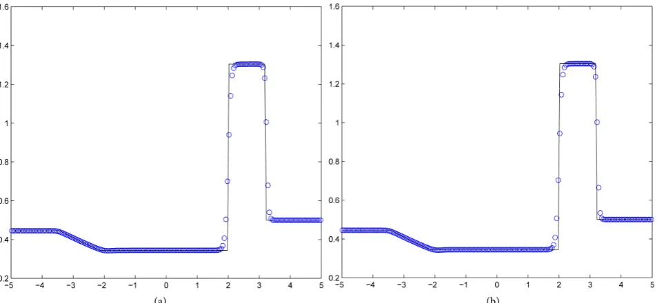
between these two schemes and they both present high-resolution results. To make further comparison, we show the l1 error and computing time in Table 2. The exact solution of Riemann problem (27) (28) is generated by the code of E. F. Toro in [19]. From this table, we can find that, with the same number of cells,

the l1 error of WENOEL-LF is slightly larger than WENOJS-LF scheme. But

the WENOEL-LF scheme only need almost one-third of the computing time compared with the WENOJS-LF scheme. Here, we also plot the relationship between the l1 error and computing time in Figure 5. Apparently, to achieve the equal error, the WENOEL-LF scheme spends less computing time than WENOJS-LF scheme.

[image:11.595.61.538.296.516.2]

(a) (b)

Figure 4. The solutions of problem (27) (28) are computed by the WENOEL-LF and WENOJS-LF methods; (a) WENOEL-LF scheme; (b) WENOJS-LF scheme.

Table 2. The comparisons of computing time (in seconds) and l1 error for the problem (27) (28) between the WENOEL-LF and WENOJS-LF methods.

WENOEL-LF WENOJS-LF

N l1 error CPU time l1 error CPU time

200 1.0707e−01 0.530 1.0513e−01 1.373

400 5.6455e−02 2.137 5.5274e−02 5.476

800 2.9261e−02 8.518 2.8725e−02 21.762

1600 1.5890e−02 34.055 1.5637e−02 86.877

3200 9.2582e−03 136.282 9.1210e−03 347.461

[image:11.595.208.538.595.734.2]

For solving the problem (27) (29), we have the same set as the previous example but with different number of cells. Because no exact solution can be

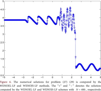
[image:12.595.210.539.127.384.2]

obtained, there is no comparison of error. In Figure 6, we show the numerical

Figure 5. The comparison of efficiency for problem (27) (28) is presented between the WENOEL-LF and WENOJS-LF methods.

Figure 6. The numerical solutions for problem (27) (29) is computed by the WENOEL-LF and WENOJS-LF methods. The “+” and “” denotes the solutions computed by the WENOEL-LF and WENOJS-LF schemes with N=400, respectively.

[image:12.595.208.537.425.721.2]

solution of the WENOJS-LF scheme with N =400 and the numerical solutions

[image:13.595.209.540.455.719.2]

of the WENOEL-LF scheme with N=400 and N=600, respectively. The

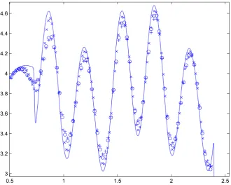
Figure 7 is the zoomed version of the Figure 6 around the high-frequency wave, From this zoomed figure, it is easily found that, with the same number of cells

400

N= , the WENOJS-LF scheme generates the solution with higher resolution

than WENOEL-LF scheme. However, the WENOJS-LF and WENOEL-LF schemes spend about 8 and 3 seconds to evolve the solutions, respectively. In addition, we present another numerical solution generated by the WENOEL-LF

scheme with N=600. This solution spends about 7 seconds and performs

clearly higher resolution. In a word, with the same computing time, the WENOEL-LF scheme can obtains the solution with higher resolution.

For the problem (27) (30), also due to there is no exact solution, we use the

same way as last example to compare these two schemes. In Figure 8, we show

the numerical solution by the WENOJS-LF scheme with N=400 and the

numerical solutions by the WENOEL-LF scheme with N =400 and N =600,

respectively. With the same number of cells, as usual, the WENOJS-LF scheme gives higher-resolution solution than the WENOEL-LF scheme, which is shown in Figure 9. The computing times needed for the WENOJS-LF and WENOEL-LF

schemes, when N=400, are about 15 and 6 seconds, respectively. If the

number of cells increases from N =400 to N=600 for the WENOEL-LF

scheme, the numerical solution has higher resolution than the WENOJS-LF

scheme which is computed with N=400. However, it is noted that the

WENOEL-LF scheme only needs 13 seconds at this time. That is, to achieve the same resolution the WENOEL-LF scheme needs much more cells, but takes less computing time.

[image:14.595.206.539.59.364.2]

Figure 8. The numerical solutions for problem (27) (30) is computed by the WENOEL-LF and WENOJS-LF methods. The “+” and “” denotes the solutions computed by the WENOEL-LF and WENOJS-LF schemes with N=400, respectively.

The “×” denotes the solutions computed by the WENOEL-LF scheme with N=600.

Figure 9. The zoomed version of Figure 8 around complicated region.

4.3. The 2D Euler System

[image:14.595.209.538.401.657.2]

(

)

(

)

2

2 0,

t x y

u v

u p uv

u

uv v p

v

E p u E p v

E

ρ ρ

ρ

ρ ρ

ρ

ρ ρ

ρ

   

 

   

  ₊

   

 _{ + + =}

   

  +

   

  _{+ +}

   

     

(31)

where the equation of state is

(

₁

)

1

(

2 2

)

_{, 1.4.}

2

p= γ− _E− ρ u +v _ γ =

 

Here, we apply the WENOEL-LF and WENOJS-LF schemes to the 2D double-Mach shock reflection problem where a strong vertical shock moves horizontally into a wedge which inclined with some angle with the ratio of

specific heats γ =1.4. Initially, this problem was proposed by Woodward and

Colella [20] and had been taken extensively as a test example for high-order

schemes. The computational domain is chosen to be

[ ] [ ]

0, 4 × 0,1 and the

reflective wall lies on the bottom of the computational domain for 1 4

6≤ ≤x . In

the beginning, a Mach 10 shock, moving right, is located at 1

6

x= , y=0 and

makes an angle 60˚ with the x-axis. For the boundary conditions, the exact

postshock condition is imposed for bottom boundary from x=0 to 1

6

x= ,

and the reflective boundary condition is imposed for the rest; the flows are imposed on the top boundary such that there is no interaction with the Mach 10 shock; inflow and outflow boundary conditions are set for the left and right boundaries respectively. The unshocked fluid has a density of 1.4, a pressure of 1 and this problem is run until t=0.2.

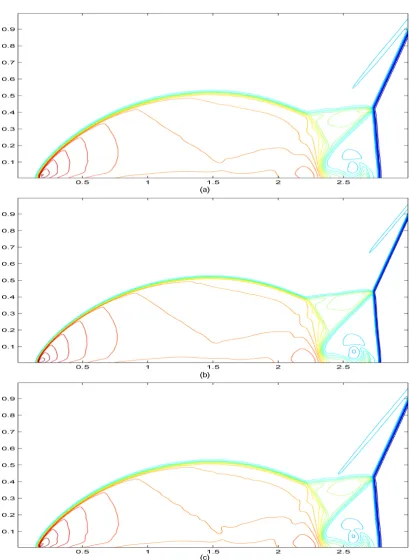
In Figure 10, we plot the numerical solution of the WENOJS-LF scheme with cells 400 × 100 and the numerical solutions of the WENOEL-LF scheme with cells 400 × 100 and 560 × 140, respectively. As the conclusion of 1D cases, with the same number of cells, the WENOJS-LF scheme can obtain higher-resolution solutions than the WENOEL-LF scheme, but with much more computing time. When we increase the number of cells from 400 × 100 to 560 × 140, the numerical solution of the WENOEL-LF scheme performs higher resolution but with almost the same computing time as the WENOJS-LF scheme with 400 × 100.

5. Conclusion

This paper aims to combine the finite volume semi-Lagrangian WENO method with flux vector splitting. The proposed scheme is rather robust and easily implemented. And the computing time of the WENOEL-LF scheme is about half and one third of the WENOJS-LF scheme in scalar equation and nonlinear system, respectively. But with the same number of cells, unlike the performance in [14], the numerical solution of WENOJS-LF scheme is slightly better than that

of WENOEL-LF scheme. If we compare the L1 error with computing time (or

[image:16.595.128.539.59.620.2]

Figure 10. Double Mach problem. (a) The density contour is computed by the WENOEL-LF scheme with 400 × 100; (b) The density contour is computed by the WENOEL-LF scheme with 560 × 140; (c) The density contour is computed by the WENOJS-LF scheme with 400 × 100. 30 equally spaced contour lines are plotted from 1.731 to 22.9705.

Acknowledgements

This work was supported by the National Natural Science Foundation of China (No. 11501238), Natural Science Foundation of Guangdong Province (No. 2012A030313119) and supported by the Major Project Foundation of Guang-dong Province Education Department (No. 2014KZDXM070).

References

[1] Staniforth, A. and Cote, J. (1991) Semi-Lagrangian Integration Schemes for At-mospheric Models—A Review. Monthly Weather Review, 119, 2206-2223.

https://doi.org/10.1175/1520-0493(1991)119<2206:SLISFA>2.0.CO;2

[2] Lin, S.J. and Rood, R.B. (1996) Multi-Dimensional Flux-Form Semi-Lagrangian Transport Schemes. Monthly Weather Review, 124, 2046-2070.

https://doi.org/10.1175/1520-0493(1996)124<2046:MFFSLT>2.0.CO;2

[3] Sonnendrucker, E., Roche, J., Bertrand, P. and Ghizzo, A. (1999) The Semi-Lagran gian Method for the Numerical Resolution of the Vlasov Equation. Journal of Computational Physics, 149, 201-220.

[4] Crouseilles, N., Mehrenberger, M. and Sonnendrucker, E. (2010) Conservative Semi-Lagrangian Schemes for Vlasov Equations. Journal of Computational Physics, 229, 1927-1953.

[5] Qiu, J.M. and Shu, C.W. (2011) Conservative Semi-Lagrangian Finite Difference WENO Formulations with Applications to the Vlasov Equation. Journal of Com-putational Physics, 10, 979-1000. https://doi.org/10.4208/cicp.180210.251110a

[6] Qiu, J.M. and Christlieb, A. (2010) A Conservative High Order Semi-Lagrangian WENO Method for the Vlasov Equation. Journal of Computational Physics, 229, 1130-1149.

[7] Liu, X.D., Osher, S. and Chan, T. (1994) Weighted Essentially Non-Oscillatory Schemes. Journal of Computational Physics, 115, 200-212.

[8] Jiang, G.S. and Shu, C.W. (1996) Efficient Implementation of Weighted ENO Schemes. Journal of Computational Physics, 126, 202-228.

[9] Arbogast, T. and Wheeler, M.F. (1995) A Characteristics-Mixed Finite Element Method for Advection-Dominated Transport Problems. SIAM Journal on Numeri-cal Analysis, 32, 404-424. https://doi.org/10.1137/0732017

[10] Qiu, J.M. and Shu, C.W. (2011) Conservative High Order Semi-Lagrangian Finite Difference WENO Methods for Advection in Incompressible Flow. Journal of Computational Physics, 230, 863-889.

[11] Arbogast, T. and Huang, C. (2006) A Fully Mass and Volume Conserving Imple-mentation of a Characteristic Method for Transport Problems. SIAM Journal on Scientific Computing, 28, 2001-2022. https://doi.org/10.1137/040621077

[12] Huang, C., Arbogast, T. and Qiu, J. (2012) An Eulerian-Lagrangian WENO Finite Volume Scheme for Advection Problems. Journal of Computational Physics, 231, 4028-4052.

[13] Huang, C. and Arbogast, T. (2017) An Eulerian–Lagrangian Weighted Essentially Nonoscillatory scheme for Nonlinear Conservation Laws. Numerical Methods for Partial Differential Equations, 33, 651-680.

[14] Sanders, R., Morano, E. and Druguet, M. (1998) Multi-Dimensional Dissipation for Upwind Schemes: Stability and Applications to Gas Dynamics. Journal of Compu-tational Physics, 145, 511-537.

Me-thods: Analysis and Cures for the “Carbuncle” Phenomenon. Journal of Computa-tional Physics, 166, 271-301.

[16] Kim, S., Kim, C., Rho, O. and Hong, S. (2003) Cures for the Shock Instability: De-velopment of a Shock-Stable Roe Scheme. Journal of Computational Physics, 185, 342-374.

[17] Lax, P.D. (1954) Weak Solutions of Nonlinear Hyperbolic Equations and Their Numerical Computation. Communications on Pure and Applied Mathematics, 7, 159-193. https://doi.org/10.1002/cpa.3160070112

[18] Toro, E.F. (2009)Riemann Solver and Numerical Methods for Fluid Dynamics. 3rd edition, Springer-Verlag, New York.

[19] Hu, F. (2017) Conservative and Easily Implemented Finite Volume Semi-Lagran gian WENO Methods for 1D and 2D Hyperbolic Conservation Laws. J. Applied Mathematics and Physics, 5, 59-82. https://doi.org/10.4236/jamp.2017.51008

[20] Woodward, P. and Colella, P. (1984) The Numerical Simulation of Two-Dimen sional Fluid Flow with Strong Shocks. Journal of Computational Physics, 54, 115- 173.

Submit or recommend next manuscript to SCIRP and we will provide best service for you:

Accepting pre-submission inquiries through Email, Facebook, LinkedIn, Twitter, etc. A wide selection of journals (inclusive of 9 subjects, more than 200 journals)

Providing 24-hour high-quality service User-friendly online submission system Fair and swift peer-review system

Efficient typesetting and proofreading procedure

Display of the result of downloads and visits, as well as the number of cited articles Maximum dissemination of your research work

Submit your manuscript at: http://papersubmission.scirp.org/