Artificial Intelligence in the Estimation of Patch Dimensions of Rectangular Microstrip Antennas

Artificial Intelligence in the Estimation of Patch

Dimensions of Rectangular Microstrip Antennas

Vandana Vikas Thakare1, Pramod Singhal2

1_{Department of Electronics and Instrumentation Engineering, Anand Engineering College, Keetham, Agra, India} 2_{Department of Electronics Engineering, Madhav Institute of Technology & Science, Gwalior, India}

E-mail: vandanavt_19@rediffmail.com

Received July 13, 2011; revised August 8, 2011; accepted August 15, 2011

Abstract

Artificial Neural Network (ANNs) techniques are recently indicating a lot of promises in the application of various micro-engineering fields. Such a use of ANNs for estimating the patch dimensions of a microstrip line feed rectangular microstrip patch antennas has been presented in this paper.An ANN model has been devel-oped and tested for rectangular patch antenna design. The performance of the neural network has been com-pared with the simulated values obtained from IE3D EM Simulator. It transforms the data containing the di-electric constant (εr), thickness of the substrate (h), and antenna’s dominant-mode resonant frequency (fr) to

the patch dimensions i.e. length (L) and width (W) of the patch. The different variants of back propagation training algorithm of MLFFBP-ANN (Multilayer feed forward back propagation Artificial Neural Network) and RBF-ANN (Radial basis function Artificial Neural Network) has been used to implement the network model. The results obtained from artificial neural network when compared with simulation results, found satisfactory and also it is concluded that RBF network is more accurate and fast as compared to different variants of back propagation training algorithms of MLPFFBP. The ANNs results are more in agreement with the simulation findings. Neural network based estimation has the usual advantage of very fast and simultaneous response of all the outputs.

Keywords:Microstrip Antenna, Bandwidth, Simulation, Modelling, Neural Networks, CAD

1. Introduction

Microstrip antennas are used in a wide range of mobile communication applications which demands multi band and/or wideband frequency operations, high power gain omni directional radiations patterns etc. Therefore design of printed antennas to meet the requirements of multiple operational services becomes a difficult task. This war-rants in the very high accuracy of the calculation of various design parameters of microstrip patch antennas. Patch dimensions of a rectangular microstrip antenna is a vital parameter in deciding the performance and the utility of an antenna. In the present work, microstrip line feeding is taken as a preferred method of feeding the input power to the antenna. The calculation of exact patch dimensions of rectangular microstrip patch antenna becomes ex-tremely important where the antenna size is drastically small. A number of papers have been appeared on the calculation of patch dimension of microstrip antennas

[1-3]. However, these papers suffer considerable deviation in the calculated value of patch dimensions compared to theoretical and simulation findings. In this paper, an at-tempt has been made to exploit the capability of artificial neural networks to calculate the length (L) and width (W) of microstrip patch antenna over a ground plane with a substrate thickness hand dielectric constants εr. The results

V. V. THAKARE ET AL. 331

authors extend the work on the use of the artificial neural network (ANN) technique taking into account different variants of back propagation training algorithm with MLPFFBP and RBF ANN model is stressed upon in place of conventional numerical techniques for the microstrip antenna design.

2. Design and Data Generation

The rectangular microstrip antennas are made up of a rectangular patch with dimensions width (W) and length (L) over a ground plane with a substrate thickness h

having dielectric constant εr. There are numerous

sub-strates that can be used for the design of microstrip an-tennas, and their dielectric constants are usually in the range of 2.2 < εr < 12. Thin substrates with higher

di-electric constants are desirable for microwave circuitry because they require tightly bound fields to minimize undesired radiation and coupling, and lead to smaller element.

The software used to model and simulate the proposed microstrip patch antenna is Zeland Inc’s IE3D software. IE3D is a full-wave electromagnetic simulator based on the method of moments. It analyses 3D and multilayer structures of general shapes. It has been widely used in the design of MICs, RFICs, patch antennas, wire antennas, and other RF/wireless antennas. It can be used to calculate and plot the S11 parameters, VSWR, current distributions as well as the radiation patterns.

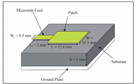
As an example microstrip line feed rectangular patch microstrip antenna is designed to resonate at 8 Ghz

fre-quency with dielectric constant (εr) = 2, substrate

thick-ness h = 1 mm, L = 12.6 mm, W = 15.3 mm. The length and the width of the patch are calculated by the given relationships. (1), (2), (3) and (4) mentioned in [15,16].

r r 2 W 2f 1     v (1) L 2f     r reff v

2 L (2)

where vis the free space velocity of the light.









W

0.3 0.264

L _0.412 h

W

h _{0.258 0.8}

h      _  _  _     _  _   reff reff

 ₍₃₎

where is extension in length due to fringing effects

and effective dielectric constant is given by

L



1/ 2 r 1 r 1 _{1 12}h

2 2 W

          _  _  

reff (4)

The transmission line model is applicable to infinite ground planes only. However, for practical considerations, it is essential to have a finite ground plane. It is known that similar results for finite and infinite ground plane can be obtained if the size of the ground plane is greater than the patch dimensions by approximately six times the substrate thickness all around the periphery. Hence, for this design, the ground plane dimensions would be given as:

Lg = 6 (h) + L = 6(1) + 12.6 = 17.6 mm (5) Wg = 6 (h) + W= 6(1) +15.3 = 21.3 mm (6) With the calculated values of various design parameters the patch antenna is designed for 8 GHz resonating fre-quency. The exact position of feed point can be deter-mined by using IE3D Electromagnetic Simulator. The

width Wo of microstrip line taken as 0.5 mm and the feed

length is 2 mm. The patch is energized electromagneti-cally using 50 ohm microstrip feed line. The geometry of

the example antenna is as shown in the Figure 1.

IE3D software has been used to calculate the return loss (S11) & hence the dominant resonating frequency of the

antenna and the data is generated in the form of fr

(reso-nating frequency) for different specified range i.e. 1.5_ εr

_ 3.5, 1 mm _h _5 mm, 11 mm _ L _ 16.5 mm and 13 mm _W _19 mm and has been used to train the various ANN model. The generated data were then arranged in five matrices. The feed coordinates and dimensions of micro-strip line are kept constant and corresponding resonating frequencies are recorded and this data has been used as a training data and test data for MLFFBP and RBF ANN. The three matrices containing the values of εr, h and fr are

used as the input to the network. The other two matrices

containing the corresponding values of L and W i.e.

length and width of the patch are the outputs of the neural network.

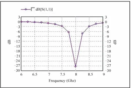
Figure 2 shows the return loss (S11) vs. frequency

curve for the given physical dimension for the example antenna indicating that antenna is resonating at 8 GHz.

Figure 2. The return loss (S11) in dB vs. resonating fre-quency of microstrip antenna.

The length, width, substrate thickness h and dielectric

constant (εr), were varied for the specified range to see

the effect on the microstrip antenna bandwidth. It was observed that antenna performance could be controlled by varying these parameters to a large extent.

3. Network Architecture and Training

For the present work three layer network MLFFBP [17,18] with 6 different training algorithms and RBF network is preferred to model the microstrip line feed patch antenna.

3.1. Multi Layer Feed Forward Back Propagation (MLFFBP)

MLP networks are feed forward networks trained with the

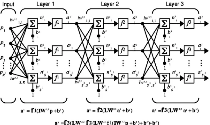
standard back propagation algorithm as shown in Figure

3. They are supervised networks and also they required a

desired response to be trained. With one or two hidden layers they can approximate virtually any input output map. The weights of the network are usually computed by training the network using the back propagation algo-rithm.

In the present work three layers multilayer perceptron feed-forward back propagation artificial neural network with one hidden layer and trained by six different variants of back propagation training algorithms is used and compared to design microstrip patch antenna.

Back propagation [17] was created by generalizing the Window-Hoff learning rule to multiple-layer networks and nonlinear differentiable transfer functions. Standard back propagation is a gradient descent algorithm, in which the network weights are moved along the negative of the gradient of the performance function.

There are many variations of the back propagation al-gorithm. The simplest implementation of back

propaga-tion learning updates the network weights and biases in the direction in which the performance function decreases most rapidly—the negative of the gradient. Six different variants of back propagation algorithm have been used to train the MLPFFBP network model developed for the proposed design.

Scaled Conjugate Gradient (SCG) This belongs to

the class of conjugate gradient methods which show super linear convergence on the most problems. This was de-signed to avoid the time consuming line approach. The algorithm is an implementation of avoiding the compli-cated line search procedure of conventional conjugate gradient algorithm

Bayesian Regularization algorithm (BR) This

algo-rithm updates the weight and bias values according to the Levenberg-Marquardt optimization and minimizes a lin-ear combination of squared errors and weight. It also modifies the linear combination so that at the end of training the resulting network has good generalization quality.

Levenberg-Marquardtoptimization algorithm (LM)

This is a least square estimation method based on the minimum neighborhood idea and does not suffer from the problem of slow convergence. The LM method combines the best feature of the Gauss Newton technique and the steepest decent method but avoid many of their limita-tions.

Quasi Newton algorithm (QN) This is based on

Newton’s method but doesn’t require calculation of sec-ond derivatives; an approximate Hessian Matrix is up-dated. At each iteration of the algorithm the update is computed as a function of gradient Conjugate.

Gradient of Fletcher Reeves algorithm (CGF) In this

algorithm a search is performed along the conjugate di-rections which produces generally faster convergence than steepest descends direction. The algorithm updates weight and biases values according to the formulas pro-posed by Fletcher and Reeves.

Adaptive Gradient Decent algorithm (AGD) It trains

any network as long as its weight, net input, and transfer functions have derivative functions. Back propagation is used to calculate derivatives of performance with respect to the weight and bias variables. Each variable is adjusted according to gradient descent.

ANN structure i.e. number of layers, number of

V. V. THAKARE ET AL. 333

Figure 3. Three layer feed forward artificial neural network.

proposed problem. The network is trained with six dif-ferent training algorithms to achieve the required degree of accuracy and hence compared for network perform-ance.

In the network there are three input neurons in the input layer, 20 hidden neurons in the hidden layer and two output neurons in the output layer. The various inputs to

the network are εr, h and fr and the outputs of the neural

network are L and W i.e. length and width of the patch.

The training time is 35 seconds and training performs in 361 epochs. In this work, different algorithms are used for training the proposed neural model and a comparative evaluation of relative performance is carried out for es-timating patch dimensions L and W of microstrip antenna. In order to evaluate the performance of proposed MLFFBP-ANN based model for the design of microstrip antenna, simulation results are obtained using IE3D Simulator and generated 120 input-output training pat-terns and 30 inputs-output test patpat-terns to validate the

model. The network has been trained for different εr, h and

fr values of the proposed example but in a specified range.

During the training process the neural network auto-matically adjusts its weights and threshold values such that the error between predicted and sampled outputs is minimized. The adjustments are computed by the back propagation algorithm. The training algorithm most suitable is trainlm .The error goal is 0.001 and learning rate is 0.1. The other network parameters used were noise factor of 0.004 and momentum factor of 0.075. The transfer function preferred is tansig in the architecture.

3.2. RBF Networks

Radial basis function network [17,18] is a feed forward

neural network with a single hidden layer that use radial basis activation functions for hidden neurons. RBF net-works are applied for various microwave modeling pur-poses. The RBF neural network has both a supervised and unsupervised component to its learning. It consists of three layers of neurons—input, hidden and output. The hidden layer neurons represent a series of centers in the input data space. Each of these centers has an activation function, typically Gaussian. The activation depends on the distance between the presented input vector and the centre. The further the vector is from the centre, the lower is the activation and vice versa. The generation of the centers and their widths is done using an unsupervised k-means clustering algorithm. The centers and widths created by this algorithm then form the weights and biases of the hidden layer, which remain unchanged once the clustering has been done. A typical RBF network struc-ture is given in Figure 4.

The parameters cijand λij are centers and standard

de-viations of radial basis activation functions. Commonly used radial basis activation functions are Gaussian and Multiquadratic. Given the inputs x, the total input to the

ith hidden neuron i is given by Equation (7).

2

1

, 1, 2,3, ,



 

  

 _ _ 

 



i

j ij x c

i N (7)

where N is the number of hidden neurons. The output

value of the ith hidden neuron is zij= σ (i) where σ (i)

is a radial basis function. Finally, the outputs of the RBF network are computed from hidden neurons as shown in Equation (8)

0 N

k ki i

y w



λij＞cij

Figure 4. Radial basis function (RBF) artificial neural net-work.

where wki is the weight of the link between the ith neuron

of the hidden layer and the kth neuron of the output layer.

Training parameters w of the RBF network include wk0,

wki, cij, λij, k = 1,2, ···, m, I = 1 ,2, ···, N, j = 1,2, ···, n.

In the RBF network, the spread value was chosen as 0.01, which gives the best accuracy. The network was trained with 120 samples and tested with 30 samples. In the structure there are 3 inputs and 2 outputs are chosen for the present synthesis ANN Model. RBF networks are more fast and effective as compared to MLPFFBP for this antenna design example. The RBF network automatically adjusts the number of processing elements in the hidden layer till the defined accuracy is reached. In the present work the RBF ANN model the network is choosing 26 processing elements in the hidden layer. The training time is 25 seconds and training performs in 212 epochs and the training algorithm is unsupervised k-means clustering algorithm.

4. Results and Conclusions

4.1. Results

It has been established from Table 1 that the

Leven-berg-Marquardt algorithm with structure (3-20-2) is the suitable model to achieve optimal values of speed of convergence and accuracy in case of MLPFFBP. It has been observed that total number of 125 epochs as shown in Figure 5 is needed to reduce MSE level to a low value

1.6e - 027 for three layers MLPFFBP. With Levenberg- Marquardt (LM) training algorithm and tansig as a transfer function achievement of such a low value of performance goal (MSE) indicates that trained ANN model with trainlm as a training algorithm is an accurate model for designing the Microstrip patch antenna. The

Figure 5. Number of epochs to achieve minimum mean square error level with Levenberg-Marquardt (LM) as a training algorithm in case of MLPFFBP.

maximum absolute error at each value of L and W (patch dimensions) antenna is estimated for the random values of input parameters but in specified range i.e. the range for which network is trained. Various transfer functions are used for training the network and average minimum MSE on training and CV data is measured. It is observed that

tansig as shown in Figure 6 is most suitable transfer

function for the present work. The MLP neural network is trained using learning rules namely Levenberg-Marquardt (LM), Scale Conjugate Gradient Back propagation (SC- GBP), Gradient of Fletcher Reeves algorithm (GFR), Quasi Newton algorithm (QN), Bayesian Regularization Algorithm (BR) and Adaptive Gradient Decent (AGD). Minimum MSE and maximum absolute error is measured

on training and test data and is indicated in Table 1 and

Figure 7. It is concluded that Levenberg- Marquaradt is

most suitable learning rule for our neural network with 3-20-2 structure. For generalization the randomized data is fed to the network and is trained for different hidden layers. It is observed that MLP with single hidden layer

gives better performance as shown in Figure 8. The

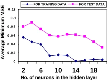
number of Processing Elements (PEs) in the hidden layer is also varied. The network is trained and minimum MSE is obtained when 20 PEs are used in hidden layer as shown in Figure 9.

As the work signifies RBF ANN is also used to model the microstrip line feed patch antenna. It is established

from Table 1 and Figure 7 that RBF is giving results not

only more accurate but fast also. The presented RBF network has performed training in only 74 epochs to the

MSE value of 6.79e-28 as shown in Figure 10. So it is

concluded that RBF architecture is better from MLPFFBP to the accuracy of 99.69% and quite faster comparatively.

4.2. Conclusions

V. V. THAKARE ET AL. 335

Table 1. Comparison of different variants of back propagation training algorithm for the design of microstrip line feed rec-tangular patch Antenna using artificial neural network.

Training algorithms _{of epochs} Number _{square error} Mean Maximum Absolute Error Estimation of length (L) Training data Test data

Estimation of (W) Maximum Absolute Error

Training data Test data

Levenberg-Marquardt (LM) 125 1.6e - 027 0.0141 0.1813 0.0227 0.1765

Scale Conjugate Gradient Back

propagation (SCGBP) 450 9.20e - 25 0.0784 0.6221 0.1334 0.4190

Gradient of Fletcher Reeves

algorithm (CGF) 640 2.65e - 13 0.1519 1.6140 0.1724 1.9992

Quasi Newton algorithm (QN) 800 8.03e - 19 0.1290 1.7645 0.1645 1.3004

Bayesian Regularization

Algorithm (BR) 590 3.67e - 20 0.1721 1.8999 0.1205 1.4143

Adaptive Gradient Decent(AGD) 485 1.77e - 026 0.0667 0.3215 0.0814 0.5216

RBF 74 6.79e - 28 0.0008 0.0748 0.0016 0.1027

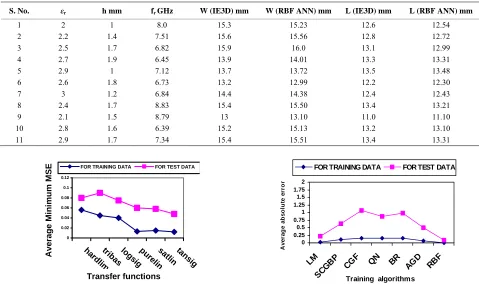
Table 2. Comparisons of results of IE3D EM simulator and RBF ANN for the calculation of patch dimensions of microstrip antenna.

S. No. εr h mm fr GHz W (IE3D) mm W (RBF ANN) mm L (IE3D) mm L (RBF ANN) mm

1 2 1 8.0 15.3 15.23 12.6 12.54

2 2.2 1.4 7.51 15.6 15.56 12.8 12.72

3 2.5 1.7 6.82 15.9 16.0 13.1 12.99

4 2.7 1.9 6.45 13.9 14.01 13.3 13.31

5 2.9 1 7.12 13.7 13.72 13.5 13.48

6 2.6 1.8 6.73 13.2 12.99 12.2 12.30

7 3 1.2 6.84 14.4 14.38 12.4 12.43

8 2.4 1.7 8.83 15.4 15.50 13.4 13.21

9 2.1 1.5 8.79 13 13.10 11.0 11.10

10 2.8 1.6 6.39 15.2 15.13 13.2 13.10

11 2.9 1.7 7.34 15.4 15.51 13.4 13.31

0 0.02 0.04 0.06 0.08 0.1 0.12

ha_rd

limtribas lo

gs_igpure

lin sa

tlintans_ig

Transfer functions

Average M

ini

m

u

m

M

S

E FOR TRAINING DATA FOR TEST DATA

Figure 6. Graph showing variation of average minimum MSE on Training and Test data set for different transfer functions in the neural network.

reader’s one of the approach to model the patch antenna using MLFFBP and RBF-ANN. The results obtained with the present technique were closer to the simulation results generated by simulating the example antenna in IE3D

Simulator. Table 1 shows the comparison of results of

different variant of back propagation algorithm of

0 0.25 0.5 0.75 1 1.25 1.5 1.75 2

LM SCG

BP _CGF QN BR

AG D

RB F

Training algorithms

A

ver

ag

e ab

so

lu

te e

rr

o

r

FOR TRAINING DATA FOR TEST DATA

Figure 7. Graph showing variation of average absolute er-ror on training and test data for different training algo-rithms

MLPFFBP ANN and RBF ANN. The paper concludes that results obtained using present ANN techniques are quite satisfactory and also that RBF ANN is giving the best approximation to the design as compared to

MLPFFBP ANN. Table 2 respectively depicts the

0 0 . 0 2 0 . 0 4 0 . 0 6 0 . 0 8 0 . 1 0 . 12

1 2 3 4 5 6 7 8 9 10

Number of hidden layers

Av

er

ag

e

M

in

im

u

m

M

S

E FOR TRAINING DATA FOR TEST DATA

Figure 8. Graph showing variation of average minimum MSE on Training and Test data set for different no. of the hidden layers in the neural network.

0 0 . 0 2 0 . 0 4 0 . 0 6 0 . 0 8 0 . 1 0 .12

2 6 10 14 18

No. of neurons in the hidden layer

A

ver

ag

e M

in

imu

m M

S

E FOR TRAINING DATA FOR TEST DATA

Figure 9. Graph showing variation of average minimum MSE on Training and Test data set for different no. of hid- den layers in the network.

Figure 10. Number of epochs to achieve minimum mean square error level with RBF ANN.

for those 11 input combinations which are not included in the set of training data and found satisfactory.

A neural network-based CAD model is developed for the design of a rectangular patch antenna, which is robust both from the angle of time of computation and accuracy. A distinct advantage of neuro computing is that, after proper training, a neural network completely bypasses the repeated use of complex iterative processes for new cases

presented to it. The developed network structure can predict the results for patch dimensions provided that the values of εr, fr and h are in the domain of training values.

5. References

[1] R. K. Mishra and A. Patnaik, “Neural Network-Based CAD Model for the Design of Square-Patch Antennas,”

IEEE Transactions on Antennas and Propagation, Vol.

46, No. 12, 1998, pp. 1890-1891. doi:10.1109/8.743842 [2] J. L. Narayan, K. Sri R. Krishna and L. P. Reddy,

“De-sign of Microstrip Antenna Using Artificial Neural Net-works,” International Conference on Computational

In-telligence and Multimedia Applications, Vol. 1, 2007, pp.

332-334.

[3] N. Turker, F. Gunes and T. Yildirim, “Artificial Neural Design of Microstrip Antennas,” Turkish Journal of

Electrical Engineering, Vol. 14, No. 3, 2006, pp. 445-

453.

[4] A. Patnaik, R. K. Mishra, G. K. Patra and S. K. Dash, “An Artificial Neural Network Model for Effective Di-electric Constant of Microstripline,” IEEE Transactions

on Antennas Propagation,Vol. 45, No. 11, 1997, p. 1697.

doi:10.1109/8.650084

[5] D. Karaboga, K. Giiney, S. Sagıroglu and M. Erler, “Neural Computation of Resonant Frequency of Electri-cally Thin and Thick Rectangular Microstrip Antennas,”

IEEE Proceedings of Microwaves, Antennas and

Propa-gation, Vol. 146, No. 2, 1999, pp. 155-159.

doi:10.1049/ip-map:19990136

[6] S. Sagiroglu, K. Guney and M. Erler, “Computation of Radiation Efficiency for a Resonant Rectangular Micro-strip Patch Antenna using Back Propagation Multilayered Perceptrons,” Journal of Electrical and Electronics, Vol. 3, 2003, pp. 663-671.

[7] Q. J. Zhang and K. C. Gupta, “Neural Networks for RF and Microwave Design,” Artech House Publishers, Lon-don, 2000.

[8] F. Peik, G. Coutts and R. R. Mansour, “Application of Neural Networks in Microwave Circuit Modelling,” 1998

IEEE Canadian Conference of Electrical and Computer

Engineering, Waterloo, 24-28 May 1998, pp. 928-931.

[9] S. Devi, D. C. Panda and S. S. Pattnaik, “A Novel Method of Using Artificial Neural Networks to Calculate Input Impedance of Circular Microstrip Antenna,”

An-tennas and Propagation Society International Symposium,

Vol. 3, 2000, pp. 462-465.

[10] R. K. Mishra and A. Patnaik, “Design of Circular Micro-strip Antenna Using Neural Networks,” IETE Journal of

Research, Vol. 44, No. 122, 1998, pp. 35-39.

[11] S. Sagiroglu and K. Guney and M. Erler, “Calculation of Resonant Frequency for an Equilateral Triangular Micro-strip Antenna Use with the of Artificial Neural Net-works,” Microwave and Optical Technology Letters, Vol. 14, No. 3, 2003, pp. 89-93.

Mi-V. Mi-V. THAKARE ET AL. 337

crowave Engineering,” IEEE Microwave Magazine, Vol. 1, 2000, pp. 55-60.

[13] M. Naser-Moghaddasi, P. D. Barjoei and A. Naghsh, “Heuristic Artificial Neural Network for Analysing and Synthesizing Rectangular Microstrip Antenna,”

Interna-tional Journal of Computer Science and Network Security,

Vol. 7, No. 12, 2007, pp. 278-281.

[14] V. V. Thakare and P. K. Singhal, “Bandwidth Analysis by Introducing Slots in Microstrip Antenna Design Using ANN,” Progress in Electromagnetic Research M, Vol. 9,

2009, pp. 107-122. doi:10.2528/PIERM09093002

[15] D. M. Pozar, “Microstrip Antennas,”John Wiley and Sons, Hoboken, 1995, pp. 79-81. doi:10.1109/5.119568

[16] C. A. Balanis, “Antenna Theory,” John Wiley & Sons, Hoboken, 1997.

[17] S. Haykin, “Neural Networks,” 2nd Edition,Prentice-Hall of India, Delhi, 2000.