Learning New Semi-Supervised Deep Auto-encoder Features
for Statistical Machine Translation
Shixiang Lu, Zhenbiao Chen, Bo Xu
Interactive Digital Media Technology Research Center (IDMTech) Institute of Automation, Chinese Academy of Sciences, Beijing, China
{shixiang.lu,zhenbiao.chen,xubo}@ia.ac.cn
Abstract
In this paper, instead of designing new fea-tures based on intuition, linguistic knowl-edge and domain, we learn some new and effective features using the deep auto-encoder (DAE) paradigm for phrase-based translation model. Using the unsupervised pre-trained deep belief net (DBN) to ini-tialize DAE’s parameters and using the in-put original phrase features as a teacher for semi-supervised fine-tuning, we learn new semi-supervised DAE features, which are more effective and stable than the unsuper-vised DBN features. Moreover, to learn high dimensional feature representation, we introduce a natural horizontal compo-sition of more DAEs for large hidden lay-ers feature learning. On two Chinese-English tasks, our semi-supervised DAE features obtain statistically significant im-provements of 1.34/2.45 (IWSLT) and 0.82/1.52 (NIST) BLEU points over the unsupervised DBN features and the base-line features, respectively.
1 Introduction
Recently, many new features have been explored for SMT and significant performance have been obtained in terms of translation quality, such as syntactic features, sparse features, and reordering features. However, most of these features are man-ually designed on linguistic phenomena that are related to bilingual language pairs, thus they are very difficult to devise and estimate.
Instead of designing new features based on in-tuition, linguistic knowledge and domain, for the first time, Maskey and Zhou (2012) explored the possibility of inducing new features in an unsuper-vised fashion using deep belief net (DBN) (Hinton et al., 2006) for hierarchical phrase-based
trans-lation model. Using the 4 original phrase fea-tures in the phrase table as the input feafea-tures, they pre-trained the DBN by contrastive divergence (Hinton, 2002), and generated new unsupervised DBN features using forward computation. These new features are appended as extra features to the phrase table for the translation decoder.
However, the above approach has two major shortcomings. First, the input original features for the DBN feature learning are too simple, the limited 4 phrase features of each phrase pair, such as bidirectional phrase translation probabil-ity and bidirectional lexical weighting (Koehn et al., 2003), which are a bottleneck for learning ef-fective feature representation. Second, it only uses the unsupervised layer-wise pre-training of DBN built with stacked sets of Restricted Boltzmann Machines (RBM) (Hinton, 2002), does not have a training objective, so its performance relies on the empirical parameters. Thus, this approach is un-stable and the improvement is limited. In this pa-per, we strive to effectively address the above two shortcomings, and systematically explore the pos-sibility of learning new features using deep (multi-layer) neural networks (DNN, which is usually re-ferred under the nameDeep Learning) for SMT.
To address the first shortcoming, we adapt and extend some simple but effective phrase features as the input features for new DNN feature learn-ing, and these features have been shown sig-nificant improvement for SMT, such as, phrase pair similarity (Zhao et al., 2004), phrase fre-quency, phrase length (Hopkins and May, 2011), and phrase generative probability (Foster et al., 2010), which also show further improvement for new phrase feature learning in our experiments.
To address the second shortcoming, inspired by the successful use of DAEs for handwrit-ten digits recognition (Hinton and Salakhutdinov, 2006; Hinton et al., 2006), information retrieval (Salakhutdinov and Hinton, 2009; Mirowski et
al., 2010), and speech spectrograms (Deng et al., 2010), we propose new feature learning using semi-supervised DAE for phrase-based translation model. By using the input data as the teacher, the “semi-supervised” fine-tuning process of DAE ad-dresses the problem of “back-propagation without a teacher” (Rumelhart et al., 1986), which makes the DAE learn more powerful and abstract features (Hinton and Salakhutdinov, 2006). For our semi-supervised DAE feature learning task, we use the unsupervised pre-trained DBN to initialize DAE’s parameters and use the input original phrase fea-tures as the “teacher” for semi-supervised back-propagation. Compared with the unsupervised DBN features, our semi-supervised DAE features are more effective and stable.
Moreover, to learn high dimensional feature representation, we introduce a natural horizontal composition for DAEs (HCDAE) that can be used to create large hidden layer representations simply by horizontally combining two (or more) DAEs (Baldi, 2012), which shows further improvement compared with single DAE in our experiments.
It is encouraging that, non-parametric feature expansion using gaussian mixture model (GMM) (Nguyen et al., 2007), which guarantees invari-ance to the specific embodiment of the original features, has been proved as a feasible feature gen-eration approach for SMT. Deep models such as DNN have the potential to be much more represen-tationally efficient for feature learning than shal-low models like GMM. Thus, instead of GMM, we use DNN (DBN, DAE and HCDAE) to learn new non-parametric features, which has the sim-ilar evolution in speech recognition (Dahl et al., 2012; Hinton et al., 2012). DNN features are learned from the non-linear combination of the input original features, they strong capture high-order correlations between the activities of the original features, and we believe this deep learn-ing paradigm induces the original features to fur-ther reach their potential for SMT.
Finally, we conduct large-scale experiments on IWSLT and NIST Chinese-English translation tasks, respectively, and the results demonstrate that our solutions solve the two aforementioned shortcomings successfully. Our semi-supervised DAE features significantly outperform the unsu-pervised DBN features and the baseline features, and our introduced input phrase features signifi-cantly improve the performance of DAE feature
learning.
The remainder of this paper is organized as fol-lows. Section 2 briefly summarizes the recent re-lated work about the applications of DNN for SMT tasks. Section 3 presents our introduced input fea-tures for DNN feature learning. Section 4 de-scribes how to learn our semi-supervised DAE fea-tures for SMT. Section 5 describes and discusses the large-scale experimental results. Finally, we end with conclusions in section 6.
2 Related Work
Recently, there has been growing interest in use of DNN for SMT tasks. Le et al. (2012) improved translation quality of n-gram translation model by using a bilingual neural LM, where transla-tion probabilities are estimated using a continu-ous representation of translation units in lieu of standard discrete representations. Kalchbrenner and Blunsom (2013) introduced recurrent contin-uous translation models that comprise a class for purely continuous sentence-level translation mod-els. Auli et al. (2013) presented a joint lan-guage and translation model based on a recur-rent neural network which predicts target words based on an unbounded history of both source and target words. Liu et al. (2013) went be-yond the log-linear model for SMT and proposed a novel additive neural networks based translation model, which overcome some of the shortcom-ings suffered by the log-linear model: linearity and the lack of deep interpretation and represen-tation in features. Li et al. (2013) presented an ITG reordering classifier based on recursive auto-encoders, and generated vector space representa-tions for variable-sized phrases, which enable pre-dicting orders to exploit syntactic and semantic information. Lu et al. (2014) adapted and ex-tended the max-margin based RNN (Socher et al., 2011) into HPB translation with force decoding and converting tree, and proposed a RNN based word topology model for HPB translation, which successfully capture the topological structure of the words on the source side in a syntactically and semantically meaningful order.
fea-tures using DNN for SMT.
3 Input Features for DNN Feature Learning
The phrase-based translation model (Koehn et al., 2003; Och and Ney, 2004) has demonstrated supe-rior performance and been widely used in current SMT systems, and we employ our implementation on this translation model. Next, we adapt and ex-tend some original phrase features as the input fea-tures for DAE feature learning.
3.1 Baseline phrase features
We assume that source phrase f = f1,· · ·, flf
and target phrase e = e1,· · · , ele includelf and
le words, respectively. Following (Maskey and
Zhou, 2012), we use the following 4 phrase fea-tures of each phrase pair (Koehn et al., 2003) in the phrase table as the first type of input fea-tures, bidirectional phrase translation probability (P(e|f)andP(f|e)), bidirectional lexical weight-ing (Lex(e|f)andLex(f|e)),
X1 →P(f|e), Lex(f|e), P(e|f), Lex(e|f)
3.2 Phrase pair similarity
Zhao et al. (2004) proposed a way of using term weight based models in a vector space as addi-tional evidences for phrase pair translation quality. This model employ phrase pair similarity to en-code the weights of content and non-content words in phrase translation pairs. Following (Zhao et al., 2004), we calculate bidirectional phrase pair simi-larity using cosine distance and BM25 distance as,
Scos
i (e, f) =
Ple
j=1Pli=1f wejp(ej|fi)wfi
sqrt(Ple
j=1we2j)sqrt(
Ple
j=1waej2)
Scos
d (f, e) = Plf
i=1 Ple
j=1wfip(fi|ej)wej
sqrt(Plf
i=1w2fi)sqrt(
Plf
i=1wafi 2
)
where, p(ej|fi) and p(fi|ej) represents
bidirec-tional word translation probability. wfi and wej
are term weights for source and target words,wej
a
andwfi
a are the transformed weights mapped from
all source/target words to the target/source dimen-sion at wordej andfi, respectively.
Sibm25(e, f) = lf
X
i=1 idffi
(k1+ 1)wfi(k3+ 1)wfai
(K+wfi)(k3+wfai)
Sbm25
d (f, e) = le
X
j=1 idfej
(k1+ 1)wej(k3+ 1)waej
(K+wej)(k3+weaj)
where, k1, b, k3 are set to be 1, 1 and 1000,
re-spectively.K=k1((1−b) +J/avg(l)), andJis
the phrase length (le orlf),avg(l)is the average
phrase length. Thus, we have the second type of input features
X2→Sicos(f, e), Sibm25(f, e), Sdcos(e, f), Sdbm25(e, f)
3.3 Phrase generative probability
We adapt and extend bidirectional phrase genera-tive probabilities as the input features, which have been used for domain adaptation (Foster et al., 2010). According to the background LMs, we esti-mate the bidirectional (source/target side) forward and backward phrase generative probabilities as
Pf(f) =P(f1)P(f2|f1)· · ·P(flf|flf−n+1,· · ·, flf−1)
Pf(e) =P(e1)P(e2|e1)· · ·P(ele|ele−n+1,· · ·, ele−1)
Pb(f) =P(flf)P(flf−1|flf)· · ·P(f1|fn,· · ·, f2)
Pb(e) =P(ele)P(ele−1|ele)· · ·P(e1|en,· · ·, e2) where, the bidirectional forward and backward1 background 4-gram LMs are trained by the corre-sponding side of bilingual corpus2. Then, we have the third type of input features
X3 →Pf(e), Pb(e), Pf(f), Pb(f)
3.4 Phrase frequency
We consider bidirectional phrase frequency as the input features, and estimate them as
P(f) = P count(f)
|fi|=|f|count(fi)
P(e) = P count(e)
|ej|=|e|count(ej)
where, thecount(f)/count(e) are the total num-ber of phrase f/e appearing in the source/target side of the bilingual corpus, and the denominator are the total number of the phrases whose length are equal to |f|/|e|, respectively. Then, we have the forth type of input features
X4 →P(f), P(e)
1Backward LM has been introduced by Xiong et al.
(2011), which successfully capture both the preceding and succeeding contexts of the current word, and we estimate the backward LM by inverting the order in each sentence in the training data from the original order to the reverse order.
2This corpus is used to train the translation model in our
3.5 Phrase length
Phrase length plays an important role in the trans-lation process (Koehn, 2010; Hopkins and May, 2011). We normalize bidirectional phrase length by the maximum phrase length, and introduce them as the last type of input features
X5 →len, lfn
In summary, except for the first type of phrase feature X1 which is used by (Maskey and Zhou,
2012), we introduce another four types of effec-tive phrase featuresX2,X3,X4andX5. Now, the
input original phrase featuresX includes 16 fea-tures in our experiments, as follows,
X →X1, X2, X3, X4, X5
We build the DAE network where the first layer with visible nodes equaling to 16, and each visible nodevicorresponds to the above original features Xin each phrase pair.
4 Semi-Supervised Deep Auto-encoder Features Learning for SMT
Each translation rule in the phrase-based transla-tion model has a set number of features that are combined in the log-linear model (Och and Ney, 2002), and our semi-supervised DAE features can also be combined in this model. In this section, we design our DAE network with various network structures for new feature learning.
4.1 Learning a Deep Belief Net
Inspired by (Maskey and Zhou, 2012), we first learn a deep generative model for feature learning using DBN. DBN is composed of multiple layers of latent variables with the first layer represent-ing the visible feature vectors, which is built with stacked sets of RBMs (Hinton, 2002).
For a RBM, there is full connectivity between layers, but no connections within either layer. The connection weight W, hidden layer biases c and visible layer biases b can be learned efficiently using the contrastive divergence (Hinton, 2002; Carreira-Perpinan and Hinton, 2005). When given a hidden layerh, factorial conditional distribution of visible layervcan be estimated by
P(v= 1|h) =σ(b+hTWT)
whereσdenotes the logistic sigmoid. Givenv, the element-wise conditional distribution ofhis
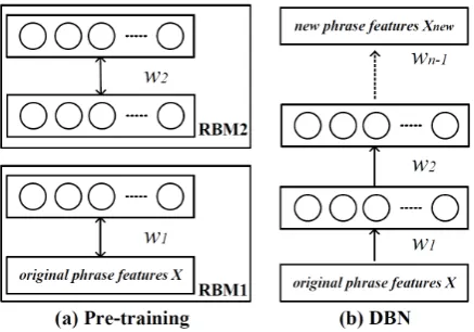
[image:4.595.308.527.62.215.2]P(h= 1|v) =σ(c+vTW)
Figure 1: Pre-training consists of learning a stack of RBMs, and these RBMs create an unsupervised DBN.
The two conditional distributions can be shown to correspond to the generative model,
P(v, h) = Z1exp(−E(v, h))
where,
Z=X
v,h
e−E(v,h)
E(v, h) =−bTv−cTh−vTW h
After learning the first RBM, we treat the acti-vation probabilities of its hidden units, when they are being driven by data, as the data for training a second RBM. Similarly, anth RBM is built on
the output of the n−1th one and so on until a
sufficiently deep architecture is created. Thesen
RBMs can then be composed to form a DBN in which it is easy to infer the states of thenth layer
of hidden units from the input in a single forward pass (Hinton et al., 2006), as shown in Figure 1. This greedy, layer-by-layer ptraining can be re-peated several times to learn a deep, hierarchical model (DBN) in which each layer of features cap-tures strong high-order correlations between the activities of features in the layer below.
To deal with real-valued input featuresXin our task, we use an RBM with Gaussian visible units (GRBM) (Dahl et al., 2012) with a variance of 1 on each dimension. Hence,P(v|h)andE(v, h)in the first RBM of DBN need to be modified as
P(v|h) =N(v;b+hTWT, I)
E(v, h) = 12(v−b)T(v−b)−cTh−vTW h
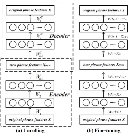
Figure 2: After the unsupervised pre-training, the DBNs are “unrolled” to create a semi-supervised DAE, which is then fine-tuned using back-propagation of error derivatives.
To speed-up the pre-training, we subdivide the entire phrase pairs (with featuresX) in the phrase table into small mini-batches, each containing 100 cases, and update the weights after each mini-batch. Each layer is greedily pre-trained for 50 epochs through the entire phrase pairs. The weights are updated using a learning rate of 0.1, momentum of 0.9, and a weight decay of 0.0002
×weight×learning rate. The weight matrixW
are initialized with small random values sampled from a zero-mean normal distribution with vari-ance 0.01.
After the pre-training, for each phrase pair in the phrase table, we generate the DBN features (Maskey and Zhou, 2012) by passing the original phrase featuresXthrough the DBN using forward computation.
4.2 From DBN to Deep Auto-encoder
To learn a semi-supervised DAE, we first “unroll” the above n layer DBN by using its weight ma-trices to create a deep, 2n-1 layer network whose lower layers use the matrices to “encode” the in-put and whose upper layers use the matrices in reverse order to “decode” the input (Hinton and Salakhutdinov, 2006; Salakhutdinov and Hinton, 2009; Deng et al., 2010), as shown in Figure 2. The layer-wise learning of DBN as above must be
treated as a pre-training stage that finds a good region of the parameter space, which is used to initialize our DAE’s parameters. Starting in this region, the DAE is then fine-tuned using average squared error (between the output and input) back-propagation to minimize reconstruction error, as to make its output as equal as possible to its input.
For the fine-tuning of DAE, we use the method of conjugate gradients on larger mini-batches of 1000 cases, with three line searches performed for each mini-batch in each epoch. To determine an adequate number of epochs and to avoid over-fitting, we fine-tune on a fraction phrase table and test performance on the remaining validation phrase table, and then repeat fine-tuning on the en-tire phrase table for 100 epochs.
We experiment with various values for the noise variance and the threshold, as well as the learn-ing rate, momentum, and weight-decay parame-ters used in the pre-training, the batch size and epochs in the fine-tuning. Our results are fairly ro-bust to variations in these parameters. The precise weights found by the pre-training do not matter as long as it finds a good region of the parameter space from which to start the fine-tuning.
The fine-tuning makes the feature representa-tion in the central layer of the DAE work much better (Salakhutdinov and Hinton, 2009). After the fine-tuning, for each phrase pair in the phrase table, we estimate our DAE features by passing the original phrase featuresX through the “encoder” part of the DAE using forward computation.
To combine these learned features (DBN and DAE feature) into the log-linear model, we need to eliminate the impact of the non-linear learning mechanism. Following (Maskey and Zhou, 2012), these learned features are normalized by the av-erage of each dimensional respective feature set. Then, we append these features for each phrase pair to the phrase table as extra features.
4.3 Horizontal Composition of Deep Auto-encoders (HCDAE)
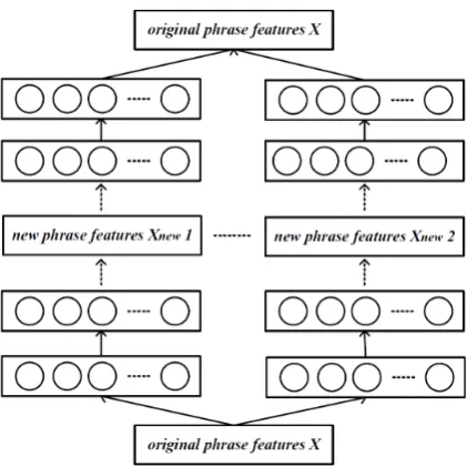
[image:5.595.73.296.59.291.2]Figure 3: Horizontal composition of DAEs to ex-pand high-dimensional features learning.
speech spectrograms (Deng et al., 2010). More-over, although we have introduced another four types of phrase features (X2,X3,X4andX5), the
only 16 features inXare a bottleneck for learning large hidden layers feature representation, because it has limited information, the performance of the high-dimensional DAE features which are directly learned from single DAE is not very satisfactory.
To learn high-dimensional feature representa-tion and to further improve the performance, we introduce a natural horizontal composition for DAEs that can be used to create large hidden layer representations simply by horizontally combining two (or more) DAEs (Baldi, 2012), as shown in Figure 3. Two single DAEs with architectures
16/m1/16 and16/m2/16can be trained and the
hidden layers can be combined to yield an ex-panded hidden feature representation of sizem1+ m2, which can then be fed to the subsequent
lay-ers of the overall architecture. Thus, these new
m1+m2-dimensional DAE features are added as
extra features to the phrase table.
Differences inm1- andm2-dimensional hidden
representations could be introduced by many dif-ferent mechanisms (e.g., learning algorithms, ini-tializations, training samples, learning rates, or distortion measures) (Baldi, 2012). In our task, we introduce differences by using different initial-izations and different fractions of the phrase table.
[image:6.595.315.518.60.193.2]4-16-8-2 4-16-8-4 4-16-16-8 4-16-8-4-2 4-16-16-8-4 4-16-16-8-8 4-16-16-8-4-2 4-16-16-8-8-4 4-16-16-16-8-8 4-16-16-8-8-4-2 4-16-16-16-8-8-4 4-16-16-16-16-8-8 6-16-8-2 6-16-8-4 6-16-16-8 6-16-8-4-2 6-16-16-8-4 6-16-16-8-8 6-16-16-8-4-2 6-16-16-8-8-4 6-16-16-16-8-8 6-16-16-16-8-4-2 6-16-16-16-8-8-4 6-16-16-16-16-8-8 8-16-8-2 8-16-8-4 8-16-16-8 8-16-8-4-2 8-16-16-8-4 8-16-16-8-8 8-16-16-8-4-2 8-16-16-8-8-4 8-16-16-16-8-8 8-16-16-16-8-4-2 8-16-16-16-8-8-4 8-16-16-16-16-8-8 16-32-16-2 16-32-16-4 16-32-16-8 16-32-16-8-2 16-32-16-8-4 16-32-32-16-8 16-32-16-8-4-2 16-32-32-16-8-4 16-32-32-16-16-8 16-32-32-16-8-4-2 16-32-32-16-16-8-4 16-32-32-32-16-16-8
Table 1: Details of the used network structure. For example, the architecture 16-32-16-2 (4 lay-ers’ network depth) corresponds to the DAE with 16-dimensional input features (X) (input layer), 32/16 hidden units (first/second hidden layer), and 2-dimensional output features (new DAE features) (output layer). During the fine-tuning, the DAE’s network structure becomes 16-32-16-2-16-32-16. Correspondingly, 4-16-8-2 and 6(8)-16-8-2 repre-sent the input features areX1andX1+Xi.
5 Experiments and Results
5.1 Experimental Setup
We now test our DAE features on the following two Chinese-English translation tasks.
IWSLT. The bilingual corpus is the Chinese-English part of Basic Traveling Expression pus (BTEC) and China-Japan-Korea (CJK) cor-pus (0.38M sentence pairs with 3.5/3.8M Chi-nese/English words). The LM corpus is the En-glish side of the parallel data (BTEC, CJK and CWMT083) (1.34M sentences). Our development set is IWSLT 2005 test set (506 sentences), and our test set is IWSLT 2007 test set (489 sentences).
NIST. The bilingual corpus is LDC4(3.4M sen-tence pairs with 64/70M Chinese/English words). The LM corpus is the English side of the paral-lel data as well as the English Gigaword corpus (LDC2007T07) (11.3M sentences). Our develop-ment set is NIST 2005 MT evaluation set (1084 sentences), and our test set is NIST 2006 MT eval-uation set (1664 sentences).
We choose the Moses (Koehn et al., 2007) framework to implement our phrase-based ma-chine system. The 4-gram LMs are estimated by the SRILM toolkit with modified Kneser-Ney
3the 4th China Workshop on Machine Translation 4LDC2002E18, LDC2002T01, LDC2003E07,
# Features Dev IWSLTTest Dev NISTTest
1 Baseline 50.81 41.13 36.12 32.59
2
X1
+DBNX1 2f 51.92 42.07∗ 36.33 33.11∗
3 +DAE X1 2f 52.49 43.22∗∗ 36.92 33.44∗∗
4 +DBNX1 4f 51.45 41.78∗ 36.45 33.12∗
5 +DAE X1 4f 52.45 43.06∗∗ 36.88 33.47∗∗
6 +HCDAEX1 2+2f 53.69 43.23∗∗∗ 37.06 33.68∗∗∗
7 +DBNX1 8f 51.74 41.85∗ 36.61 33.24∗
8 +DAE X1 8f 52.33 42.98∗∗ 36.81 33.36∗∗
9 +HCDAEX1 4+4f 52.52 43.26∗∗∗ 37.01 33.63∗∗∗
10
X
+DBNX 2f 52.21 42.24∗ 36.72 33.21∗
11 +DAE X 2f 52.86 43.45∗∗ 37.39 33.83∗∗
12 +DBNX 4f 51.83 42.08∗ 34.45 33.07∗
13 +DAE X 4f 52.81 43.47∗∗ 37.48 33.92∗∗
14 +HCDAEX 2+2f 53.05 43.58∗∗∗ 37.59 34.11∗∗∗
15 +DBNX 8f 51.93 42.01∗ 36.74 33.29∗
16 +DAE X 8f 52.69 43.26∗∗ 37.36 33.75∗∗
17 +HCDAEX 4+4f 52.93 43.49∗∗∗ 37.53 34.02∗∗∗
18 +(X2+X3+X4+X5) 52.23 42.91∗ 36.96 33.65∗
19 +(X2+X3+X4+X5)+DAEX 2f 53.55 44.17+∗∗∗ 38.23 34.50+∗∗∗
20 +(X2+X3+X4+X5)+DAEX 4f 53.61 44.22+∗∗∗ 38.28 34.47+∗∗∗
21 +(X2+X3+X4+X5)+HCDAE X 2+2f 53.75 44.28+∗∗∗∗ 38.35 34.65+∗∗∗∗
22 +(X2+X3+X4+X5)+DAEX 8f 53.47 44.19+∗∗∗ 38.26 34.46+∗∗∗
[image:7.595.88.517.61.409.2]23 +(X2+X3+X4+X5)+HCDAE X 4+4f 53.62 44.29+∗∗∗∗ 38.39 34.57+∗∗∗∗
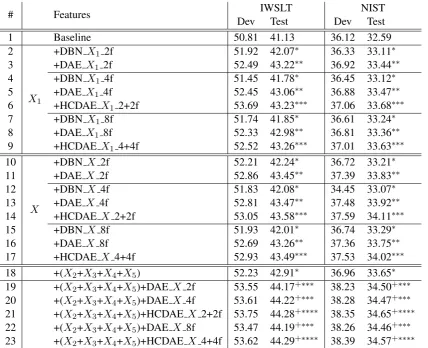
Table 2: The translation results by adding new DNN features (DBN feature (Maskey and Zhou, 2012), our proposed DAE and HCDAE feature) as extra features to the phrase table on two tasks. “DBN X1 xf”,
“DBN X xf”, “DAE X1 xf” and “DAE X xf” represent that we use DBN and DAE, input features X1 and X, to learn x-dimensional features, respectively. “HCDAE X x+xf” represents horizontally
combining two DAEs and each DAE has the same x-dimensional learned features. All improvements on two test sets are statistically significant by the bootstrap resampling (Koehn, 2004). *: significantly better than the baseline (p < 0.05), **: significantly better than “DBN X1 xf” or “DBN X xf” (p < 0.01),
***: significantly better than “DAEX1 xf” or “DAEX xf” (p <0.01), ****: significantly better than
“HCDAE X x+xf” (p <0.01), +: significantly better than “X2+X3+X4+X5” (p <0.01).
discounting. We perform pairwise ranking opti-mization (Hopkins and May, 2011) to tune feature weights. The translation quality is evaluated by case-insensitive IBM BLEU-4 metric.
The baseline translation models are generated by Moses with default parameter settings. In the contrast experiments, our DAE and HCDAE fea-tures are appended as extra feafea-tures to the phrase table. The details of the used network structure in our experiments are shown in Table 1.
5.2 Results
Table 2 presents the main translation results. We use DBN, DAE and HCDAE (with 6 layers’ net-work depth), input featuresX1 andX, to learn 2-,
4- and 8-dimensional features, respectively. From the results, we can get some clear trends:
1. Adding new DNN features as extra features significantly improves translation accuracy (row 2-17 vs. 1), with the highest increase of 2.45 (IWSLT) and 1.52 (NIST) (row 14 vs. 1) BLEU points over the baseline features.
Features σ IWSLT NIST
1 σ2 σ3 σ4 σ1 σ2 σ3 σ4
DBN X1 4f 0.1678 0.2873 0.2037 0.1622 0.0691 0.1813 0.0828 0.1637
DBN X 4f 0.2010 0.1590 0.2793 0.1692 0.1267 0.1146 0.2147 0.1051 DAE X1 4f 0.5072 0.4486 0.1309 0.6012 0.2136 0.2168 0.2047 0.2526
[image:8.595.98.506.62.145.2] [image:8.595.74.528.189.406.2]DAE X 4f 0.5215 0.4594 0.2371 0.6903 0.2421 0.2694 0.3034 0.2642 Table 3: The variance distributions of each dimensional learned DBN feature and DAE feature on the two tasks.
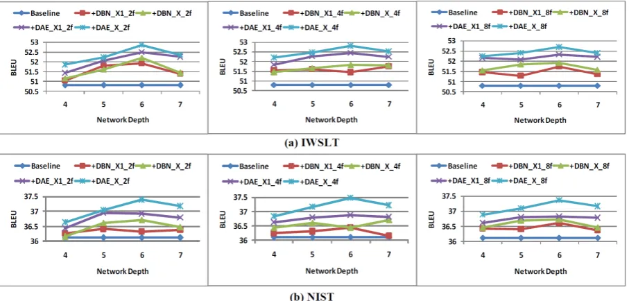
Figure 4: The compared results of feature learning with different network structures on two development sets.
Features DevIWSLTTest DevNISTTest +DAEX1 4f 52.45 43.06 36.88 33.47 +DAEX1+X2 4f 52.76 43.38∗ 37.28 33.80∗ +DAEX1+X3 4f 52.61 43.27∗ 37.13 33.66∗ +DAEX1+X4 4f 52.52 43.24∗ 36.96 33.58∗ +DAEX1+X5 4f 52.49 43.13∗ 36.96 33.56∗ +DAEX 4f 52.81 43.47∗ 37.48 33.92∗ Table 4: The effectiveness of our introduced in-put features. “DAE X1+Xi 4f” represents that
we use DAE, input featuresX1+Xi, to learn
4-dimensional features. *: significantly better than “DAE X1 4f” (p <0.05).
our DAE features have more discriminative power, and also their variance distributions are more sta-ble.
3. HCDAE outperforms single DAE for high dimensional feature learning (row 6 vs. 5; row 9 vs. 8; row 14 vs. 13; row 17 vs. 16), and further improve the performance of DAE feature learning,
which can also somewhat address the bring short-coming of the limited input features.
4. Except for the phrase feature X1 (Maskey
and Zhou, 2012), our introduced input features
X significantly improve the DAE feature learn-ing (row 11 vs. 3; row 13 vs. 5; row 16 vs. 8). Specially, Table 4 shows the detailed effectiveness of our introduced input features for DAE feature learning, and the results show that each type of features are very effective for DAE feature learn-ing.
5. Adding the original features (X2,X3,X4and X5) and DAE/HCDAE features together can
[image:8.595.82.300.464.573.2]fea-tures are complementary to the original feafea-tures.
[image:9.595.72.302.97.388.2]5.3 Analysis
Figure 5: The compared results of using single DAE and the HCDAE for feature learning on two development sets.
Figure 4 shows our DAE features are not only more effective but also more stable than DBN features with various network structures. Also, adding more input features (X vs. X1) not only
significantly improves the performance of DAE feature learning, but also slightly improves the performance of DBN feature learning.
Figure 5 shows there is little change in the per-formance of using single DAE to learn different dimensional DAE features, but the 4-dimensional features work more better and more stable. HC-DAE outperforms the single HC-DAE and learns high-dimensional representation more effectively, espe-cially for the peak point in each condition.
Figures 5 also shows the best network depth for DAE feature learning is 6 layers. When the net-work depth of DBN is 7 layers, the netnet-work depth of corresponding DAE during the fine-tuning is 13 layers. Although we have pre-trained the corre-sponding DBN, this DAE network is so deep, the fine-tuning does not work very well and typically finds poor local minima. We suspect this leads to the decreased performance.
6 Conclusions
In this paper, instead of designing new features based on intuition, linguistic knowledge and do-main, we have learned new features using the DAE for the phrase-based translation model. Using the unsupervised pre-trained DBN to initialize DAE’s parameters and using the input original phrase fea-tures as the “teacher” for semi-supervised back-propagation, our semi-supervised DAE features are more effective and stable than the unsuper-vised DBN features (Maskey and Zhou, 2012). Moreover, to further improve the performance, we introduce some simple but effective features as the input features for feature learning. Lastly, to learn high dimensional feature representation, we introduce a natural horizontal composition of two DAEs for large hidden layers feature learning.
On two Chinese-English translation tasks, the results demonstrate that our solutions solve the two aforementioned shortcomings successfully. Firstly, our DAE features obtain statistically sig-nificant improvements of 1.34/2.45 (IWSLT) and 0.82/1.52 (NIST) BLEU points over the DBN fea-tures and the baseline feafea-tures, respectively. Sec-ondly, compared with the baseline phrase features
X1, our introduced input original phrase features X significantly improve the performance of not only our DAE features but also the DBN features. The results also demonstrate that DNN (DAE and HCDAE) features are complementary to the original features for SMT, and adding them to-gether obtain statistically significant improve-ments of 3.16 (IWSLT) and 2.06 (NIST) BLEU points over the baseline features. Compared with the original features, DNN (DAE and HCDAE) features are learned from the non-linear combi-nation of the original features, they strong cap-ture high-order correlations between the activities of the original features, and we believe this deep learning paradigm induces the original features to further reach their potential for SMT.
Acknowledgments
References
Michael Auli, Michel Galley, Chris Quirk and Geoffrey Zweig. 2013. Joint language and translation
model-ing with recurrent neural networks. InProceedings
of EMNLP, pages 1044-1054.
Pierre Baldi. 2012. Autoencoders, unsupervised
learn-ing, and deep architectures. JMLR: workshop on
un-supervised and transfer learning, 27:37-50. Miguel A. Carreira-Perpinan and Geoffrey E. Hinton.
2005. On contrastive divergence learning. In
Pro-ceedings of AI and Statistics.
George Dahl, Dong Yu, Li Deng, and Alex Acero. 2012. Context-dependent pre-trained deep neural networks for large vocabulary speech recognition.
IEEE Transactions on Audio, Speech, and Language Processing, 20(1):30-42.
Li Deng, Mike Seltzer, Dong Yu, Alex Acero, Abdel-rahman Mohamed, and Geoffrey E. Hinton. 2010. Binary coding of speech spectrograms using a deep
auto-encoder. In Proceedings of INTERSPEECH,
pages 1692-1695.
George Foster, Cyril Goutte, and Roland Kuhn. 2010. Discriminative instance weighting for domain adap-tation in statistical machine translation. In Proceed-ings of EMNLP, pages 451-459.
Geoffrey E. Hinton. 2002. Training products of
ex-perts by minimizing contrastive divergence. Neural
Computation, 14(8):1771-1800.
Geoffrey E. Hinton, Li Deng, Dong Yu, George Dahl, Abdel-rahman Mohamed, Navdeep Jaitly, Andrew Senior, Vincent Vanhoucke, Patrick Nguyen, Tara Sainath, and Brian Kingsbury. 2012. Deep neural networks for acoustic modeling in speech
tecogni-tion. IEEE Signal Processing Magazine,
29(6):82-97.
Geoffrey E. Hinton, Alex Krizhevsky, and Sida D.
Wang. 2001. Transforming auto-encoders. In
Pro-ceedings of ANN.
Geoffrey E. Hinton and Ruslan R. Salakhutdinov. 2006. Reducing the dimensionality of data with neural networks. Science, 313:504-507.
Geoffrey E. Hinton, Simon Osindero, and Yee-Whye Teh. 2006. A fast learning algorithm for deep belief
nets. Neural Computation, 18:1527-1544.
Mark Hopkins and Jonathan May 2011. Tuning as
ranking. In Proceedings of EMNLP, pages
1352-1362.
Nal Kalchbrenner and Phil Blunsom. 2013.
Recur-rent continuous translation models. InProceedings
of EMNLP, pages 1700-1709.
Philipp Koehn. 2004. Statistical significance tests
from achine translation evaluation. InProceedings
of ACL, pages 388-395.
Philipp Koehn. 2010. Statistical machine translation.
Cambridge University Press.
Philipp Koehn, Hieu Hoang, Alexandra Birch, Chris Callison-Burch, Marcello Federico, Nicola Bertoldi, Brooke Cowan, Wade Shen, Christine Moran, Richard Zens, Chris Dyer, Ondrej Bojar, Alexandra Constantin, and Evan Herbst. 2007. Moses: Open source toolkit for statistical machine translation. In
Proceedings of ACL, Demonstration Session, pages 177-180.
Philipp Koehn, Franz J. Och, and Daniel Marcu. 2003. Statistical phrase-based translation. InProceedings of NAACL, pages 48-54.
Hai-Son Le, Alexandre Allauzen, and Franc¸ois Yvon. 2012. Continuous space translation models with
neural networks. InProceedings of NAACL, pages
39-48.
Peng Li, Yang Liu, Maosong Sun. 2013. Recursive autoencoders for ITG-based translation. In Proceed-ings of EMNLP, pages 567-577.
Lemao Liu, Taro Watanabe, Eiichiro Sumita, and Tiejun Zhao. 2013. Additive neural networks for
statistical machine translation. In Proceedings of
ACL, pages 791-801.
Shixiang Lu, Wei Wei, Xiaoyin Fu and Bo Xu. 2014. Recursive neural network based word topology model for hierarchical phrase-based speech transla-tion. InProceedings of ICASSP.
Yuval Marton and Philip Resnik. 2008. Soft syntactic constraints for hierarchical phrase-based translation. InProceedings of ACL, pages 1003-1011.
Sameer Maskey and Bowen Zhou. 2012. Unsuper-vised deep belief features for speech translation. In
Proceedings of INTERSPEECH.
Piotr Mirowski, MarcAurelio Ranzato, and Yann Le-Cun. 2010. Dynamic auto-encoders for semantic
indexing. InProceedings of NIPS-2010 Workshop
on Deep Learning.
Patrick Nguyen, Milind Mahajan, and Xiaodong He. 2007. Training non-parametric features for
statis-tical machine translation. InProceedings of WMT,
pages 72-79.
Franz J. Och and Hermann Ney. 2000. Improved
sta-tistical alignment models. In Proceedings of ACL,
pages 440-447.
Franz J. Och and Hermann Ney. 2002. Discriminative training and maximum entropy models for statistical
machine translation. InProceedings of ACL, pages
295-302.
Franz J. Och and Hermann Ney. 2004. The alignment template approach to statistical machine translation.
David Rumelhart, Geoffrey E. Hinton, and Ronale Williams. 1986. Learning internal representations
by back-propagation errors. Parallel Distributed
Processing, Vol 1: Foundations, MIT Press. Ruslan R. Salakhutdinov and Geoffrey E. Hinton.
2009. Semantic hashing. International Journal of
Approximate Reasoning, 50(7):969-978.
Richard Socher, Cliff C. Lin, Andrew Y. Ng, and Christopher D. Manning. 2011. Parsing natural scenes and natural language with recursive neural
networks. InProceedings of ICML.
Deyi Xiong, Min Zhang, and Haizhou Li. 2011. Enhancing language models in statistical machine translation with backward n-grams and mutual
in-formation triggers. In Proceedings of ACL, pages
1288-1297.
Bing Zhao, Stephan Vogel, and Alex Waibel. 2004. Phrase pair rescoring with term weightings for
sta-tistical machine translation. In Proceedings of