Leveraging Loyalty Programs Using Competitor Based Targeting

Munich Personal RePEc Archive

Leveraging Loyalty Programs Using

Competitor Based Targeting

Hollenbeck, Brett and Taylor, Wayne

UCLA Anderson, SMU Cox

2019

Online at

https://mpra.ub.uni-muenchen.de/92900/

Leveraging Loyalty Programs Using Competitor Based

Targeting

Wayne Taylor

Cox School of Business

Southern Methodist University

∗

Brett Hollenbeck

Anderson School of Management

UCLA

†

March 11, 2019

Abstract

Loyalty programs are widely used by firms but their effectiveness is subject to debate.

These programs provide discounts and perks to loyal customers and are costly to administer,

and with uncertain effectiveness at increasing spending or stealing business from rivals. We use

a large new dataset on retail purchases before and after joining a loyalty program (LP) at the

customer level to evaluate what determines LP effectiveness. We exploit detailed spatial data on

customer and store locations, including locations of competing firms. A simple analysis shows

that location relative to competitors is the strongest predictor of LP effectiveness, suggesting

that LPs work primarily through business stealing and not through other demand expansion.

We next estimate what variables best predict LP effectiveness using high-dimensional data on

spatial relationships between customers, the focal firm’s stores, and competing stores as well

as customers’ historical spending patterns. We use LASSO regularization to show that spatial

relationships are more predictive of LP effects than are past sales data. Finally, we show

how firms can use this type of predictive analytics model to leverage customer and competitor

location data to substantially increase the performance of their LP through spatially driven

targeting rules.

Keywords: Loyalty programs, predictive analytics, spatial models, retail competition, machine

learn-ing

∗

[email protected]

1

Introduction

Loyalty programs are now prevalent in many industries. The loyalty programs as marketers know

them today originated in the airlines in the 1980s and have since permeated industries such as

hotels, casinos, retailers, grocery stores, and restaurants, among others. The pervasiveness of

loyalty programs is partly due to their flexibility in how they can be structured (e.g., earning rates

and rewards) and managed for strategic decisions (e.g., targeting to increase customer engagement).

In spite of the popularity of loyalty programs with firms, their effectiveness at increasing profits

has long been subject to debate. This debate has centered on the costs of giving discounts and perks

to the most loyal customers, as well as the costs of administering the program itself, and whether

these costs are justified by increases in spending by those customers. Loyalty programs have the

potential to increase profits by increasing switching costs for existing customers, stealing business

from rivals, or through second degree price discrimination. They may also indirectly increase profits

by increasing customers psychological perceptions of the firm, by generating customer data that can

be used for targeted promotions or CRM, or by exploiting agency issues such as flights booked by

business travelers and paid for by their employers (Dreze and Nunes (2008), Roehm et al. (2002),

Verhoef (2003), and Shugan (2005)).

1

Empirical studies of whether loyalty programs actually do increase profits have found mixed

results. Verhoef (2003) finds that the effects are positive but very small, DeWulf et al. (2001) finds

no support for positive effects of direct mail, Shugan (2005) finds that firms gain short term revenue

at the expense of longer term reward payments, and Hartmann and Viard (2008) found no evidence

that loyalty programs create switching costs.

In this paper, we consider whether and when loyalty programs are profitable and to what

extent this profitability results from stealing business from rivals or increasing overall demand via

one of the mechanisms described above. We approach this problem in a novel way using a large

and detailed dataset on retail spending. We observe spending before and after customers join a

loyalty program and exploit variation across markets with different levels of competition and types

of competitors. This comparison can be made at a granular level using detailed information on

customer and competitor location. By measuring how total spending changes at the customer level

for customers facing different local competitive structures we can observe, for instance, if customers

1

For a more complete review, please see Bijmolt et al. (2011), Liu and Yang (2009), and McCall and Voorhees

in more isolated markets change their spending or if they merely start receiving discounts on their

purchases and how this differs in highly competitive markets. This type of variation can help resolve

the question of when LPs are profitable and to what extent do they work through business stealing

versus other demand expansion.

We use a large and detailed dataset that results from merging credit card spending data with

customer data from a leading retailer to show that the local competitive structure is more

pre-dictive of how customers respond to joining an LP then are their historical spending patterns. In

particular, an individual’s spatial relationship with competitor stores is the main determinant of

LP effectiveness in simple comparisons. This suggests that the loyalty program is working through

business stealing and does not otherwise raise demand. To our knowledge, this is the first paper to

explicitly link the competitive structure of a market with the performance of a loyalty program.

While model-free comparisons suggest spatial competitive structure is the crucial determinant

of LP effectiveness, the full relationship is likely to be highly complex. To capture the complex

spatial relationship between the customer, focal firm, and competition, we estimate the relationship

between the change in spending (conditional a customer on joining the LP) and a very large number

of variables on purchase data and spatial relationships with competitors at the individual level.

This estimation is essentially a prediction problem with a very large number of potential predictive

relationships. Our estimation procedure therefore combines LASSO regularization with a selection

correction approach to allow for many potential variables and to infer the true impact of spatial

structure and other variables on loyalty program performance.

This estimation serves two purposes. First, it validates the descriptive result that spatial

com-petitive structure is a stronger predictor of LP effectiveness than are past spending patterns or

other RFM variables. Second, we then use the output to show how firms can take advantage of this

insight and leverage customer and competitor location data to increase the performance of their

LP through spatially driven targeting rules. Because location and travel costs form an important

part of preferences over retailers, this can be thought of as a strategy for targeting price discounts

on observable preference heterogeneity. The variation across customers in the profitability of their

joining the LP is large, with 49.1% of joiners resulting in a net loss to the firm, suggesting the gains

from improving targeting can be quite high. We find that, consistent with the spirit of recent work

in targeting (e.g., Ascarza (2018)), firms should focus on the customers who are more “spatially

have limited access to their competitors.

The field of economics, and then later marketing, has a long history of incorporating location

effects, dating back to the study of how location with respect to competitors determines market

power (e.g., Hotelling (1929)), including empirical studies of how firms strategically employ and

respond to spatial differentiation (Seim (2006), Davis (2006), Thomadsen (2007)). This includes

research studying how market characteristics influence a firm’s price and promotion activity (Hoch

et al. (1995) and Bronnenberg and Mahajan (2001)).

Recent work has explored the benefits of geotargeting, where promotion or other marketing

activity is a function of a customer’s real-time location using mobile data (Luo et al. (2014), Chen

et al. (2016)). Fong et al. (2015) and Dube et al. (2017) have also considered “geoconquesting”,

where the marketing activity focuses on instances when the customer is located near a competitor

as opposed to near the focal firm. This literature is limited, but potential gains from geoconquesting

are especially likely when the marketing activity is based in part on business stealing, as it is for

loyalty programs. One contribution of this paper is to point out the potential gains from orienting

promotional activity towards geoconquesting, even in a non-mobile setting.

While the previous literature therefore incorporates select spatial components, mostly it does

not fully account for the complex customer-store-competitor spatial relationship. In prior work,

competitor information is often integrated into models through simple customer-store or

store-competitor distance metrics, thereby eliminating the possibility of complex spatial analyses. Beyond

complex spatial analysis alone, the interplay between the competitive structure and loyalty program

effectiveness has not yet been explored.

We also contribute to the study of competitive promotions and competitive price discrimination.

Price discrimination strategies such as loyalty rewards should never lower profits by a monopolist

but in oligopoly settings this is no longer true as firms may face a prisoner’s dilemma (Shaffer and

Zhang (1995)). Chen et al. (2001) shows that when individual targeting is possible but imperfect,

it can soften price competition among competing firms, but as targeting precision increases the

prisoner’s dilemma reasserts itself. Ultimately then, it is an empirical question whether and when

targeted price discrimination can increase profits. Previous work has shown that in practice the

benefits of using targeted pricing can be quite high (Rossi et al. (1996), Besanko et al. (2003)). Li

et al. (2018) specifically consider competitive price discrimination across markets and show that

competitive intensity across markets. Our analysis also considers local market structure but with

price discounts in the form of a loyalty program that can be targeted at the individual level.

The remainder of the paper proceeds as follows. Section 2 describes the data on retail sales

histories and competitor and customer locations. Section 3 provides model free evidence that the

spatial competitive structure surrounding a customer is the key determinant of LP effectiveness.

Section 4 describes a LASSO estimation of the complex interaction between competitive structure

and LP effectiveness and then uses this result to form a potential targeting strategy. Section 5

discusses managerial implications and avenues for future research.

2

Data

In this section we describe the customer transaction data, competitive location data, and provide

an overview of the spatial metrics used to characterize the competitive structure.

2.1

Transaction Data

The transaction data comes from a Fortune 500 specialty retailer, one of the 10 largest retailers in

the U.S. This data is highly detailed: we observe the full basket of purchases from 10,029 customers

between March 2012 and March 2014. These sum to over 2.4 million SKU level purchases across

897,819 store trips. On average, each customer has about 90 trips across nearly five different store

locations through the two year observation period, spending about $110 per store visit, and traveling

about 5.7 miles.

Customers

10,029

Date range

March 2012 to 2014

Avg. trips/customer

90

Spend/trip (net, after discounts)

$110.18

Average # of locations visited

4.7

Table 1: Summary Statistics

loyalty program card. This allows us to observe transaction activity both before and after the

customer joins the loyalty program. We also observe all marketing activity for these customers

through the firm’s email campaigns: over 900,000 emails were sent to about 39% of the customers

and 11% of the customers received promotions specifically encouraging enrollment in the loyalty

program.

Importantly, the data also contains the customer’s location and the latitude/longitude of each

of the firm’s store locations, which provides us with a complete picture of all customer interactions

with the firm across different store locations as well as the specific products purchased at each store

location over time.

We further take advantage of a unique feature of this loyalty program in that the program

discounts are earned and applied on only a single large category of the firm’s goods. We label this

a

limited

loyalty program to emphasize the distinct structure. As requested by the firm providing

the data, we cannot disclose the type of goods subject to discounts. However, because this firm

competes with both generalists, who also sell a large variety of categories, and specialists, who

only sell the products in the specific category the LP applies to, this feature provides an additional

lever with which to study the interaction between competitive structure and LP effectiveness. It

also allows us to study whether and when the loyalty program causes spillovers into other category

purchases.

2.2

Competitor Data

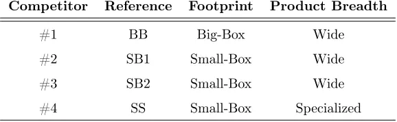
The competitor data contains the locations of four primary competitors of interest, who were

selected based on discussions with the focal firm. The four competitors (see Table 2) vary in both

size and product breadth. Competitor #1 is a big box store with a wide product variety (BB). The

remaining three competitors are small-box stores. Competitor #2 and competitor #3 offer a wide

assortment of products (SB1 and SB2), whereas competitor #4 specializes in the product category

Competitor

Reference

Footprint

Product Breadth

#1

BB

Big-Box

Wide

#2

SB1

Small-Box

Wide

#3

SB2

Small-Box

Wide

#4

SS

Small-Box

Specialized

Table 2: Competitor Types

The variety in the size and product breadth allows us to compare how the impact of the

compet-itive structure might be competitor or type specific. More importantly, it allows us to gain insight

into the extent of category-level versus store-level business stealing.

The latitude and longitude locations of each competitor are collected from the Google Maps

API. We first pulled all competitors within a 30 mile radius of each of the focal stores, and then

pulled all competitors within 30 miles of each customer located within a 30 mile radius of each focal

store. This expanded footprint ensures that our definition of the competitive structure is customer

centric rather than limited to the perspective of the focal store.

2.3

Quantifying the Competitive Structure

Our analysis measures and highlights the impact of the complex spatial relationship between the

customer, the focal store, and the competitors on customer behavior and ultimately firm profits.

Quantifying this relationship in such a way to accurately reflect the tradeoffs that an individual

likely encounters when deciding which store to visit requires several complex considerations.

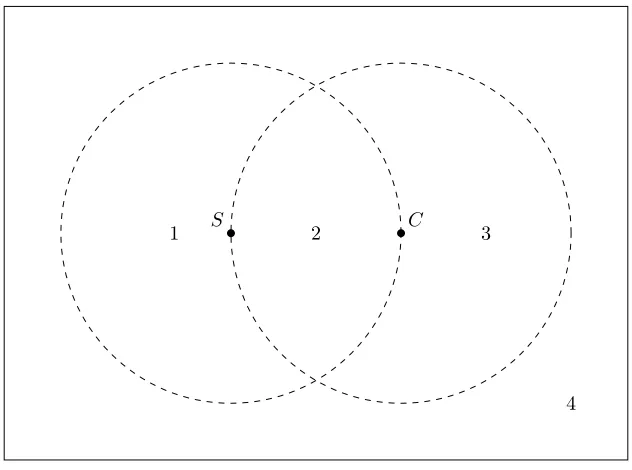
A common approach in quantifying competitive structure is to simply use the distance between

a focal store and the customer along with the distance between the competitor and the focal store

(or more commonly still, an indicator variable if they are both within, say, a 5 mile radius of the

focal store). The drawback of this approach is that it does not jointly consider the

customer-store-competitor location, resulting in a potential homogenization of very distinct competitive structures.

This limitation is illustrated in Figure 1: two competitors,

C

1

and

C

2

, and a customer,

I

, are

customer has to pass by the focal store in order to visit the first competitor,

C

1

, which suggests

some spatial advantage for the focal store. However, the second competitor,

C

2

is positioned right

next to the customer, acting as a convenient alternative to the focal store. One goal of this analysis

is to incorporate these complex spatial structures into the manager decision process, a strategy that

has heretofore been ignored in the analyses of loyalty program effectiveness.

S

C

1

C

2

I

Figure 1: Limitation of Radii Approach

We recognize that it is unreasonable to expect a single metric to capture the complex nature of

the spatial relationship between the customer, focal store, and competitor in its entirety. Instead,

we approach the problem by proposing a large number of distance metrics, each of which captures

at least some of the complex spatial relationship on its own, and then in our empirical analysis

uncover which metrics or which interactions between metrics best characterize customer behavior.

By honing in on the right combination of distance metrics we can determine which

specific

features

of the spatial relationship influence customer behavior the most.

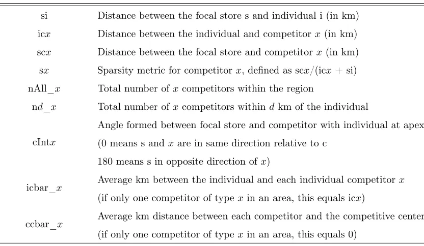
We therefore consider standard distance metrics between each customer and competitor with

the the focal firm in addition to the following:

• How much closer is the focal store to the customer, relative to the competitor?

• How

sparse

is the focal store and competitor, relative to the customer?

extent?

We also allow for interactions between population density and distance metrics to incorporate

the difference in transportation costs between urban and rural areas. For brevity, the complete

description of the distance metrics considered are contained in the appendix.

3

Spatial Competitive Structure and LP Performance

We first provide model free evidence that the spatial competitive structure, and hence business

stealing, are key determinants of LP performance. Our analysis focuses on two metrics of LP

effectiveness: the probability that a customer joins the program, and the change in average monthly

spend for customers who decide to join. Here and throughout the paper, we use the change in

spending net of the LP discounts. For customers who join the LP but do not change shopping

patterns, this change is negative by default because of the discounts and a positive change for this

metric can therefore be taken as strictly beneficial for the retailer. In this section we look at how

these metrics relate to the the distance between the customer and the focal store and the four

competitor types.

One challenge in analyzing LP effectiveness is that the customer’s decision to join the loyalty

program may be related to unobserved heterogeneity. While we observe purchases both before and

after each customer joins the LP, which allows us to condition on individual-level fixed effects, it is

still true that if customers join due to anticipated changes in their level of spending, the estimated

change in behavior attributed to the loyalty program may be over-estimated. We accommodate

this possibility in three ways. First, we assume that the location of each customer is essentially

exogenous prior to joining the LP, in which case the difference in spending across customers with

respect to the spatial relationship between the customer, the focal store, and the competition still

provide valid comparisons. Second, when we estimate a full model of the LP in the following

section, we use exclusion restrictions combined with a control function approach to account for

this unobserved heterogeneity. Finally, we replicate our results using only spending that does not

qualify for the LP discounts and is thus not potentially biased by selection on unobservables.

Descriptive Analysis:

We first examine the role of competitive structure on LP effectiveness in a transparent

in monthly spending under four possible competitive structures (as illustrated in Figure 2): (1)

when the focal store is within five miles of the customer and the competition is not, (2) when both

the focal store and the competition are within five miles of the customer, (3) when the competition

is within five miles of the customer and the focal store is not, and (4) when neither the focal store

or the competition are within five miles of the customer.

2

Table 3 shows average outcomes in each competitive structure. For customers relatively close to

the focal store (regions 1 and 2), the change in spending after joining the LP is significantly higher

than for those who are not located near the focal store (regions 3 and 4). Customers in regions 1

and 2 increase their spending by $22 per month compared to essentially no change in spending for

customers in regions 3 and 4.

Interestingly, for customers in region 1 (that is, when the focal store is relatively isolated), the

probability of joining the LP is the highest, but the change in spend at these stores for customer

that join the LP is negligible. This is intuitive: if there are no relevant competitors nearby it is

likely that the focal store already has the majority of this customer’s share of wallet.

However, in the second region when the customer has access to both the focal store and the

competition, the change in spend is very high at $80 per month. These customers may have been

splitting their purchases across stores and consolidate activity to the focal store upon joining the

loyalty program. Customers in this region are driving the entire result that customers near the

focal store significantly increase their spending. This is true despite the fact that they represent

under one quarter of the customers near the focal store. A naive analysis of spatial effects that

compared customers in region

1 + 2

to those outside it would miss this distinction.

Region 3 stands out as an outlier in the opposite direction. This region has the smallest share of

customers, and those customers have the lowest sales pre LP, the lowest join rate, and display a large

negative change in spending after joining. This change is almost entirely in non-qualified spending

and this group also exhibits a large decrease in trip frequency after joining. One interpretation is

that customers located near a competitor likely join the LP after the decision has been made to

shift non-qualified spending to the competition, and use the LP solely for the qualified spending

discounts. They then shop at the focal store much less often and only for the qualified category.

2

To be clear, a single focal store can be in multiple categories, since it depends on the relationship with respect

S

C

1

2

3

4

Figure 2: Competitive Structure Illustration

Region

Pr(Join)

∆

Sales|Join

∆

Non-Qual Sales|Join

n

Join

∆

Trip Freq

1+2

4.2%

$22

$13

429

-0.05

3+4

4.0%

-$2

-$24

487

-0.01

1

4.2%

$4

-$7

328

-0.13

2

4.1%

$80

$79

101

0.22

3

3.6%

-$85

-$82

87

-0.67

4

4.0%

$16

-$11

400

0.13

Table 3: Region Effects

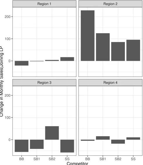
To understand what is driving these findings we break down the results by competitor type.

Figure 3 shows the average change in monthly spending, and how it varies by both competitive

structure and type of competitor. As shown previously, the largest gains are when both the

com-petitor and focal store are near the customer, which presents the most likely scenario for business

suggesting this is the most profitable firm to steal business from.

Region 3 Region 4

Region 1 Region 2

BB SB1 SB2 SS BB SB1 SB2 SS

0 100 200

0 100 200

Competitor

Change in Monthly Sales|Joining LP

Figure 3: Change in Monthly Spend by Competitor Type

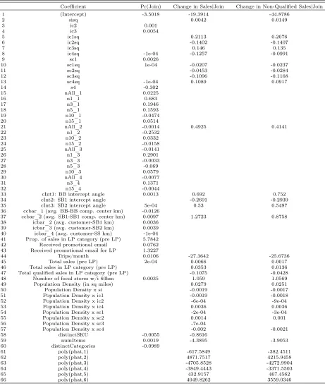
To better understand this mechanism, recall that the LP only applies to a specific large category

and not all products, and that one of the competitors (SS) specializes in selling only that category.

We thus highlight the portion of change in spend that occurs in the LP category of interest.

Figure 4 shows how spending changes across competitor types within each region for this category.

Interestingly, the changes are driven in large part by purchases outside of the category for which the

loyalty program applies. If there was no spillover effects of the loyalty program, we would expect

zero change in purchases that will not impact the LP rewards. Upon joining the LP, customers may

decide to consolidate purchase behavior with one store rather than cherry picking rewards from the

focal store (in the qualifying category) and continuing with the same purchase patterns at other

Region 3 Region 4

Region 1 Region 2

BB SB1 SB2 SS BB SB1 SB2 SS 0

100 200

0 100 200

Competitor

Change in Monthly Sales|Joining LP

Purchase Cat.

LP Excluded LP Qualified

Figure 4: Change in Monthly Spend by Competitor Type and Purchase Category

4

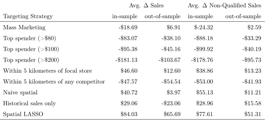
LASSO Regularization and Competitive Targeting

In this section we propose an approach that accounts for the complex spatial interaction of

compet-itive structure on LP effectiveness. This serves two purposes. First, we can analyze the estimation

results directly to evaluate the relative importance of competitive structure and traditional

predic-tors of LP effectiveness like sales histories as well as simple measures of customer location. Second,

the estimation provides a ready-made targeting strategy for a firm seeking to improve LP

effective-ness by providing predictions of which customers are the most profitable to target based on their

spending histories, precise locations, and unique competitive structures. The wide variation across

customers in profitability suggests the gains from targeting the program can be quite large.

We combine two stages of estimation to estimate the impact of the competitive structure on

program, conditional on the competitive structure. Then, we model the change in spending

con-ditional on participating in the LP in addition to the competitive structure. We estimate in two

stages to allow the competitive structure to influence the join probabilities and changes in spend

differently, and to control for self-selection into the LP.

The goal of the estimation is to predict which customers are likely to be profitable as members of

the LP based on their past sales and spatial characteristics. Because the goal is prediction and the

data are high-dimensional, the problem is well-suited to statistical methods built around dimension

reduction or “regularization.” We ultimately use a LASSO approach because this will allow us to

test inclusion of a large number of possible spatial measures and let the model select the most

predictive variables. The output also provides a clearer interpretation than other methods and one

goal of the analysis is to assess which individual factors best predict LP effectiveness.

4.1

First Stage: Probability of Joining and Selection Bias

Let the indirect utility of joining the firm’s loyalty program for customer

i

at focal store

s

be

u

is

=

β

′

X

is

+

δ

′

Z

is

+

ε

is

(1)

Here

X

contains all the distance metrics (specific to each customer-store combination) and

Z

contains firm-level marketing and store-specific customer purchase behavior.

X

is

contains the

competitive structure parameters between customer

i

at focal store location

s

. These metrics are

intended to jointly capture the complex spatial relationships between the customer, focal store, and

competitors. Since there can be more than one focal store in the vicinity of an individual, these

metrics vary across each store

s

for a given individual

i

. Likewise, since each customer’s location is

unique, the spatial metrics also vary across each individual

i

from all observations for store

s

.

β

reflects the impact of the competitive structure on an individual’s likelihood of joining the

program. We avoid specific interpretations within this vector of coefficients (e.g. representing the

cost of transportation) and instead interpret the coefficients as holistically capturing the many

spatial factors that a customer considers before committing to the firm’s loyalty program (e.g.,

convenience of the focal store relative to the competition, isolation of the focal store, distance to

the store versus other competitors, etc.).

fre-quency, overall sales, distinct number of items, number of product categories, basket size, discounts

received, sales in the category of interest, and sales in the category of interest for those products

that are included in the limited LP. In preparation for our second stage model on the change in

monthly spend, we also include variables in

Z

is

that will be used to control for selection bias,

dis-cussed in further detail below.

Z

is

therefore contains proportion of sales in the category of interest,

an indicator for whether the customer received marketing activity specifically encouraging joining

the LP, and an indicator for whether the customer received any marketing promotion.

To satisfy the exclusion restriction, these variables need to influence the probability of joining

the loyalty program but not influence the change in spending upon joining the program. We argue

that these variables satisfy the exclusion restriction, primarily because our dependent variable is

the

change

in spend with the focal store, rather than spend alone. While these variables could be

correlated with spending levels, it is unlikely there is a relationship between these

Z

variables and

change in spend upon joining the LP other than through the direct effects of the LP.

δ

captures the effects of the marketing and past purchase behavior on the utility received from

joining the loyalty program. For instance, if a large proportion of spend is already dedicated to the

category for which the LP benefits, it seems natural that the customer would be more inclined to

join the LP.

The error term

ε

is

captures the idiosyncratic variation in utility across customers and stores.

Assuming the

{

ε

is

}

are independent and identically distributed Type I extreme value, we can derive

the join probabilities as follows:

Pr (

j

i

= 1|

X

is

, Z

is

, β, δ

) =

exp (

β

′

X

is

+

δ

′

Z

is

)

1 + exp (

β

′

X

is

+

δ

′

Z

is

)

(2)

where

j

i

= 1

if customer

i

joins the limited loyalty program at some point during the observed

data.

4.2

Second Stage: Change in Spend

In the second stage we model the change in monthly store-level spend, conditional on joining the

loyalty program. Let

y

is

be the

change

in monthly sales for customer

i

at store

s

. We model this

y

is

=

γ

′

X

is

+

κ

′

Z

is

∗

+

φ

(ˆ

p

is

) +

η

is

(3)

where

η

is

is an unobserved, normally distributed random error centered at zero. Here

X

is

is

defined in the same way as in the first stage model and

Z

∗

is

is the same as

Z

is

but with the three

selection variables removed. We predict changes in store-level spend (rather than changes in

firm-level spend) to recognize that changes may be dependent on the spatial relationship a customer has

with an individual store’s location. In other words, the change in spend for an individual customer

may depend on which specific competitors are located in the vicinity of a given store location.

A common issue in analyzing the effectiveness of loyalty programs is that of self-selection.

Individuals are not randomly assigned to participate in loyalty programs, rather they choose to

be in the loyalty program for a variety of reasons. Because of this self-selection, estimates of LP

effectiveness may be upward biased. For example, those who join are more likely to spend more,

regardless of whether they are in the LP or not, so comparing the spending amounts of those who

join with those that do not capture differences in spending patterns, not the effectiveness of the LP.

We are able to mostly eliminate this concern using data containing spending both before and

after the customer joins the program. While this captures most unobserved heterogeneity, there

is still potentially the issue that the customer may have joined because of anticipated increases in

spending over time. As with before, this may lead the analyst to incorrectly believe that the loyalty

program is causing a large increase in spend when the change may have been due to this unobserved

heterogeneity.

We employ a Heckman-style two-stage correction method in an attempt to correct any remaining

selection bias. First we estimate the join probabilities using the first stage specification above,

including variables that serve as plausible exclusion restrictions. Then, we take the estimated join

probabilities for each observation and include them in the second stage model of change in spend as

a control function. Our approach is to place a flexible function

φ

over

p

ˆ

using high-order polynomials

to control for unobserved heterogeneity.

3

3

See Heckman (1979) for an introduction to the two-stage estimator and Ahn and Powell (1993) for extensions to

4.3

LASSO Estimation

Our proposed model contains a large number of spatial variables defined to capture the competitive

structure. On the one hand, capturing the spatial relationship between the customer, focal store,

and competitors is complex and may require many variables. However, all else being equal a concise

model is preferable from a managerial standpoint. In addition, many of the spatial metrics we

devised may be redundant or highly correlated with each other. To systematically remove variables

that are either unnecessary or redundant we employ the Least Absolute Shrinkage and Selection

Operator (LASSO) estimator, introduced by Frank and Friedman (1993) and Tibshirani (1996).

In general, for a model with a

k

-dimensional parameter vector

θ

the LASSO method performs

the following:

(

θ

∗

) = arg min

(

−

log

L

(

θ

) +

λ

X

k

|

θ

k

|

)

(4)

Where

L

is the likelihood of data given the model specified, and

λ

is a tuning parameter that

represents the penalty incurred if we choose a nonzero value for any parameter

θ

k

. This approach

regulates the trade-off between an accurate model with more predictive power and a concise model

that is more readily interpretable by managers.

4

We select the tuning parameter

λ

through ten

fold cross-validation, which is perhaps the simpliest and most widely used method for this task.

5

4.4

Estimation Results

The results from the LASSO estimation are presented in Table 4. For model validation purposes,

we split the original data into a 75% training set and 25% test set. The results presented below

were estimated using the training set alone. For brevity, the table only displays variables that

are significant in at least one of the two models (with the exception of the coefficients on the

control function polynomials). First we discuss how the competitive structure influences the join

probabilities before discussing the estimated impact on the change in monthly spending, as both are

4

An alternative approach would be a ridge regression or similar method. In this case the penalty is applied more

smoothly, shrinking coefficients on highly correlated variables towards each other. We prefer the LASSO approach

because the penalty structure removes coefficients entirely, resulting in clearer model interpretation. Specifically, we

can see that many non-spatial variables will drop out altogether. This direct interpretation of the model’s results is a

key output of interest. A ridge regression would lack this clean interpretation but would result in similar quantitative

predictions and can be provided upon request.

influenced differently. From a statistical standpoint, it is relatively easy to interpret the marginal

effects of each the variables. However, we must emphasize that many of the spatial impacts are

codependent and interpreting the marginal effect of one coefficient while holding another spatial

variable constant is sometimes impossible. Later, we present stylized heatmaps to better understand

the impact of the spatial relationships on change in spend.

4.4.1

Join Probabilities

The logistic regression results are shown in Table 4, and the full list of spatial variable definitions

is provided in Table 7. In this first model many of the traditional distance metrics drop out of the

model (e.g., direct distance between the focal store and the customer) in favor of secondary spatial

metrics.

For instance, as the angle between the big box competitor (BB) increases, the probability of

joining the LP at the focal store also increases. This indicates that the probability of joining

increases if the competitor is in the opposite direction relative to the customer, rather than in the

same direction. This effect also holds for the small box specialist (SS).

The last two sets of spatial components (ccbar and icbar) are designed to account for differences

in markets with the presence of multiple competitors of the same type. The first of these variables,

ccbar, is the average distance between each competitor and its competitive center (defined as

the average latitude and longitude across competitors of the same type). A relatively high value

indicates that the competitors are relatively spread out in a market. The negative coefficient on

the big box generalist (ccbar_1) indicates that the more dispersed these stores are in a market,

the less likely the customer is to join the LP. The second variable, icbar, measures the average

distance between each customer and each of the competitors. While a customer may be close to

the competitive center, a high value of icbar indicates that each individual competitor (of a given

type) is still relatively far away. This coefficient is positive for the two small-box generalists (SB1

and SB2), suggesting that a relatively sparse distribution of these competitors may be beneficial to

the focal firm.

Finally, we consider the variables used to correct for potential selection bias. First, we see a

strong positive effect on the proportion of sales in the category of interest: customers who dedicate

a greater portion of store spend to the LP category are more likely to benefit from the LP discounts.

emails and those specifically designed to enroll them in the LP.

4.4.2

Change in Monthly Spend

In this section we now review the influence of the competitive structure on the estimated LP

effectiveness, as measured by change in monthly spending at the focal store, conditional on joining

the firm’s loyalty program. Before discussing the spatial effects, we first review the results from the

selection correction. To correct for selection bias, we include up to the sixth order polynomials on

the predicted join probabilities from the previous stage. In our original LASSO regularization none

of these variables were significant, suggesting that selection resulting from unobserved heterogeneity

is not a substantial driver of the change in spending. However, in the results presented we explicitly

incorporate these variables at the cost of out-of-sample performance in order to properly control

for potential selection on unobservables.

Recall the dependent variable in this estimation is the change in monthly spend after joining the

loyalty program, net of any LP discounts. For this table, we only included customers who had at

least some spending both before and after joining. Since we are interested in how spending

changes

after joining, rather than

whether

spending occurs or not, this seems to be a reasonable filter.

First, there is a positive impact on the squared distance between the customer and the focal

store, suggesting that the greater gains come from those located further away from the focal store.

This aligns with our previous intuition: customers located near the focal store are more likely to

already dedicate the majority of their spend with the focal store, so the potential for increases in

spend are limited, relative to those who are further away and thus more likely to be sharing spend

with the competition.

Importantly, the distance between the customer and the competition also influences changes in

spend at the focal store. Customers who exhibit the largest changes in spend are those who are

relatively far from the the big-box generalist (ic1sq) and the second small-box generalist (ic3sq)

and close to from the other competitors, holding all other variables constant.

Many of the radius band coefficients drop out of this model. However, we see that the intercept

angle is retained. The difference in the estimated change in spend for a customer where a big-box

(BB) competitor is in the same line of travel as the focal store (intercept angle of zero) versus in the

opposite direction (intercept angle of 180 degrees) is about $125, holding all other variables constant.

it is important to again point out that many of these distance metrics cannot vary independently

of others. The heatmaps presented later will illustrate the degree to which the intercept angle

influences the change in spend while simultaneously accounting for other changes.

Finally, population density along with its interactions with the direct distance measures has a

significant impact on the change in monthly spend. On its own, the effect is positive: more densely

populated areas are associated with a greater change in spend. This is intuitive as more densely

populated areas tend to have a greater level of competition and higher incomes. There are also

numerous interactions with our simple distance metrics. For instance, increases in the distance

between the store and the customer influence customers in dense areas more negatively, relative

to customers in less dense areas. This appears to be capturing the challenges of traveling in more

densely populated areas (e.g., traveling a given distance in a city versus a rural setting).

As an important robustness check, we also include a column where the estimation proceeds as

before but only using the change in spending on products that do not qualify for the LP discounts.

Recall that the specific concern regarding unobserved heterogeneity was a correlation between

decision to join the LP and planned changes in spending over time related to the LP discounts.

Because these discounts do not apply to the non-qualified categories, the concern about unobserved

heterogeneity does not apply here either. Comparing this column and the column for all spending

shoes a very high correlation in the LASSO coefficients and perfect correlation in which variables

are retained. This adds further evidence that selection on unobserved heterogeneity does not have

a meaningful effect on our results.

4.4.3

Summary

The LASSO results suggest that the customer behavior appears to be influenced by the competitive

structure of the local market. The regularization tends to keep quite a few of the spatial metrics,

suggesting that relatively simple distance metrics are, on their own, unable to fully characterize the

predicted behavior. This is not very surprising: there are many intuitive reasons why a customer

may change their spending patterns after joining a loyalty program with respect to their location.

4.5

Visual Representation of Results

Even after variable reduction via LASSO, it is still difficult to interpret the spatial forces at play

Table 4: Lasso Pr(Join) and Change in Sales|Join

Coefficient

Pr(Join)

Change in Sales|Join

Change in Non-Qualified Sales|Join

1

(Intercept)

-3.5018

-19.3914

-44.8786

2

sisq

0.0042

0.0149

3

ic2

0.001

4

ic3

0.0054

5

ic1sq

0.2113

0.2076

6

ic2sq

-0.1402

-0.1407

7

ic3sq

0.146

0.135

8

ic4sq

-1e-04

-0.1257

-0.0991

9

sc1

0.0026

10

sc1sq

1e-04

-0.0207

-0.0237

11

sc2sq

-0.0453

-0.0284

12

sc3sq

-0.1096

-0.1168

13

sc4sq

-1e-04

0.1089

0.0917

14

s4

-0.302

15

nAll_1

0.0225

16

n1_1

0.683

17

n3_1

0.1946

18

n5_1

0.1593

19

n10_1

-0.0474

20

n15_1

0.0514

21

nAll_2

-0.0014

0.4925

0.4141

22

n1_2

-0.2532

23

n10_2

0.0332

24

n15_2

-0.0158

25

nAll_3

-0.0141

26

n1_3

0.2901

27

n3_3

-0.0033

28

n5_3

-0.069

29

n10_3

0.0579

30

nAll_4

-0.0077

31

n3_4

0.1371

32

n15_4

-0.0044

33

cInt1: BB intercept angle

0.0013

0.692

0.752

34

cInt2: SB1 intercept angle

-0.2691

-0.2939

35

cInt3: SB2 intercept angle

5e-04

0.53

0.5497

36

ccbar_1 (avg. BB-BB comp. center km)

-0.0126

37

ccbar_2 (avg. SB1-SB1 comp. center km)

0.0097

1.2723

0.8758

38

icbar_2 (avg. customer-SB1 km)

0.0036

39

icbar_3 (avg. customer-SB2 km)

0.0039

40

icbar_4 (avg. customer-SS km)

-1e-04

41

Prop. of sales in LP category (pre LP)

5.7842

42

Received promotional email

0.0762

43

Received promotional email for LP

1.3227

44

Trips/month

0.0106

-27.3642

-25.6736

45

Total sales (pre LP)

2e-04

0.0066

0.0017

46

Total sales in LP category (pre LP)

0.0353

0.0136

47

Total qualified sales in LP category (pre LP)

-0.1075

-0.0428

48

Number of focal stores w/i 60km

0.0035

1.059

1.0569

49

Population Density (in sq miles)

0.0279

0.0251

50

Population Density x si

-0.0019

-0.0017

51

Population Density x ic1

-0.0019

-0.0018

52

Population Density x ic2

-6e-04

-9e-04

53

Population Density x ic4

0.0036

0.0036

54

Population Density x sc1

-2e-04

-3e-04

55

Population Density x sc2

0.0014

0.001

56

Population Density x sc3

-7e-04

57

Population Density x sc4

-0.002

-0.0021

58

distinctSKU

-0.0055

-0.8616

59

numItems

0.0019

-4.3895

-3.9053

60

distinctCategories

-0.0989

61

poly(phat,1)

-617.5849

-382.4511

62

poly(phat,2)

4871.7517

4215.9458

63

poly(phat,3)

-4705.8528

-4272.9904

64

poly(phat,4)

-3849.4443

-3371.5503

65

poly(phat,5)

432.9157

467.4562

LASSO’s results on how the competitive structure influences LP effectiveness. To do so, we show

the predicted change in spending for hypothetical customers and represent the results in a series

of heatmaps showing different competitive structures. These maps show how there is large

hetero-geneity across different customers with different competitive structures in the potential gains from

having them join the LP.

Six heatmaps are presented in Figure 5. The color on the heatmap reflects the estimated change

in spend from a customer in that position if they were to join the focal store’s loyalty program.

Heatmaps (a), (b), (c), and (d) illustrate the differences between the four competitor types, keeping

the relative position between the focal store and competitor the same. The fifth heatmap (e), plots

all four competitors on a single map, each an equal distance from the focal store. Finally, the last

heatmap (f) draws a random observation from the data to illustrate the predicted effects from an

actual competitive structure. Since these maps are mostly stylized representations of the actual

data we focus on comparing the magnitudes across maps rather than specific prediction levels.

In the first heatmap (a), the greatest change in sales is from customers who are located in

between the big-box generalist (BB) and the focal store, suggesting that changes in spend are

primarily driven by shifting store spend away from the competition. The second heatmap shows

a slightly different pattern. First, we notice that the overall magnitude in predicted changes is

reduced, suggesting that any potential gains from the first small-box generalist (SB1) are relatively

limited. Here again most of the gains are coming from those directly between the focal store and

competitor, but unlike the big-box store there is not as stark of a dropoff in spend once customers

move outside of the direct path between the focal store and this competitor.

For the second small-box generalist (SB2), the effect appears to mimic the first competitor

(BB) at a slightly reduced magnitude. Again we see the strongest gains from those located directly

between the focal store and competition, but this slowly drops off as customer move further outside

of the direct line of travel.

In the fourth heatmap (d), the small-box specialist (SS) displays a pattern unique to the other

three competitors. Recall that this competitor specializes in selling the same products that qualify

for the focal store’s loyalty program. In this map customers located near the competitor exhibit the

lowest changes in spend. This suggests that taking business from this competitor may be difficult

if the focal customer are located nearby.

simul-taneously. This shows that most of the gains are from customers near the big-box generalist, and

less so from the small-box specialist. This map highlights that the value of a potential customer is

heavily dependent on the extent to which the focal store can steal business from the competition.

Finally, the last heatmap presents the predicted change in spend from an actual market structure

in the data. Customers located on the far side of the second small-box specialist (SB2), and the

big-box generalist (BB), have the lowest predicted change in spend. These customers are relatively

far away from the focal store with a competitor directly in their path of travel, resulting in limited

predicted gains. On the other hand, the other two competitors (SB1 and SS) are relatively close

and the line of travel is not as critical with these competitors. The customers that show the most

promise are those that are relatively close to the focal store but in the direction of the second small

box generalist (SB2) and the big-box generalist (BB). To be clear, this will not necessarily always

be true: the positioning of the competitors relative to the focal store (or their absence from the

market) dictates which customers are likely to contribute to the greatest changes in spend once

they join the loyalty program.

The heatmaps presented highlight two key advantages of this analysis. First, the geographic

influence of a competitor is relatively complex. Simple radii surrounding either the competitor or

the focal store may not sufficiently capture the influence of the competitive structure on customer

behavior. Second, these complex relationships are not fixed and can vary by the type of competitor

in an area. This is an important consideration for the firm in the formation of targeting

strate-gies: the combined relationship between the location of each competitor, customer, and focal store

● ● ● ● ● ● ● ● ● ● ● ● ● ● ● ● ● ● ● ● ● ● ● ● ● ● ● ● ● ● ● ● ● ● ● ● ● ● ● ● ● ● ● ● ● ● ● ● ● ● ● ● ● ● ● ● ● ● ● ● ● ● ● ● ● ● ● ● ● ● ● ● ● ● ● ● ● ● ● ● ● ● ● ● ● ● ● ● ● ● ● ● ● ● ● ● ● ● ● ● ● ● ● ● ● ● ● ● ● ● ● ● ● ● ● ● ● ● ● ● ● ● ● ● ● ● ● ● ● ● ● ● ● ● ● ● ● ● ● ● ● ● ● ● ● ● ● ● ● ● ● ● ● ● ● ● ● ● ● ● ● ● ● ● ● ● ● ● ● ● ● ● ● ● ● ● ● ● ● ● ● ● ● ● ● ● ● ● ● ● ● ● ● ● ● ● ● ● ● ● ● ● ● ● ● ● ● ● ● ● ● ● ● ● ● ● ● ● ● ● ● ● ● ● ● ● ● ● ● ● ● ● ● ● ● ● ● ● ● ● ● ● ● ● ● ● ● ● ● ● ● ● ● ● ● ● ● ● ● ● ● ● ● ● ● ● ● ● ● ● ● ● ● ● ● ● ● ● ● ● ● ● ● ● ● ● ● ● ● ● ● ● ● ● ● ● ● ● ● ● ● ● ● ● ● ● ● ● ● ● ● ● ● ● ● ● ● ● ● ● ● ● ● ● ● ● ● ● ● ● ● ● ● ● ● ● ● ● ● ● ● ● ● ● ● ● ● ● ● ● ● ● ● ● ● ● ● ● ● ● ● ● ● ● ● ● ● ● ● ● ● ● ● ● ● ● ● ● ● ● ● ● ● ● ● ● ● ● ● ● ● ● ● ● ● ● ● ● ● ● ● ● ● ● ● ● ● ● ● ● ● ● ● ● ● ● ● ● ● ● ● ● ● ● ● ● ● ● ● ● ● ● ● ● ● ● ● ● ● ● ● ● ● ● ● ● ● ● ● ● ● ● ● ● ● ● ● ● ● ● ● ● ● ● ● ● ● ● ● ● ● ● ● ● ● ● ● ● ● ● ● ● ● ● ● ● ● ● ● ● ● ● ● ● ● ● ● ● ● ● ● ● ● ● ● ● ● ● ● ● ● ● ● ● ● ● ● ● ● ● ● ● ● ● ● ● ● ● ● ● ● ● ● ● ● ● ● ● ● ● ● ● ● ● ● ● ● ● ● ● ● ● ● ● ● ● ● ● ● ● ● ● ● ● ● ● ● ● ● ● ● ● ● ● ● ● ● ● ● ● ● ● ● ● ● ● ● ● ● ● ● ● ● ● ● ● ● ● ● ● ● ● ● ● ● ● ● ● ● ● ● ● ● ● ● ● ● ● ● ● ● ● ● ● ● ● ● ● ● ● ● ● ● ● ● ● ● ● ● ● ● ● ● ● ● ● ● ● ● ● ● ● ● ● ● ● ● ● ● ● ● ● ● ● ● ● ● ● ● ● ● ● ● ● ● ● ● ● ● ● ● ● ● ● ● ● ● ● ● ● ● ● ● ● ● ● ● ● ● ● ● ● ● ● ● ● ● ● ● ● ● ● ● ● ● ● ● ● ● ● ● ● ● ● ● ● ● ● ● ● ● ● ● ● ● ● ● ● ● ● ● ● ● ● ● ● ● ● ● ● ● ● ● ● ● ● ● ● ● ● ● ● ● ● ● ● ● ● ● ● ● ● ● ● ● ● ● ● ● ● ● ● ● ● ● ● ● ● ● ● ● ● ● ● ● ● ● ● ● ● ● ● ● ● ● ● ● ● ● ● ● ● ● ● ● ● ● ● ● ● ● ● ● ● ● ● ● ● ● ● ● ● ● ● ● ● ● ● ● ● ● ● ● ● ● ● ● ● ● ● ● ● ● ● ● ● ● ● ● ● ● ● ● ● ● ● ● ● ● ● ● ● ● ● ● ● ● ● ● ● ● ● ● ● ● ● ● ● ● ● ● ● ● ● ● ● ● ● ● ● ● ● ● ● ● ● ● ● ● ● ● ● ● ● ● ● ● ● ● ● ● ● ● ● ● ● ● ● ● ● ● ● ● ● ● ● ● ● ● ● ● ● ● ● ● ● ● ● ● ● ● ● ● ● ● ● ● ● ● ● ● ● ● ● ● ● ● ● ● ● ● ● ● ● ● ● ● ● ● ● ● ● ● ● ● ● ● ● ● ● ● ● ● ● ● ● ● ● ● ● ● ● ● ● ● ● ● ● ● ● ● ● ● ● ● ● ● ● ● ● ● ● ● ● ● ● ● ● ● ● ● ● ● ● ● ● ● ● ● ● ● ● ● ● ● ● ● ● ● ● ● ● ● ● ● ● ● ● ● ● ● ● ● ● ● ● ● ● ● ● ● ● ● ● ● ● ● ● ● ● ● ● ● ● ● ● ● ● ● ● ● ● ● ● ● ● ● ● ● ● ● ● ● ● ● ● ● ● ● ● ● ● ● ● ● ● ● ● ● ● ● ● ● ● ● ● ● ● ● ● ● ● ● ● ● ● ● ● ● ● ● ● ● ● ● ● ● ● ● ● ● ● ● ● ● ● ● ● ● ● ● ● ● ● ● ● ● ● ● ● ● ● ● ● ● ● ● ● ● ● ● ● ● ● ● ● ● ● ● ● ● ● ● ● ● ● ● ● ● ● ● ● ● ● ● ● ● ● ● ● ● ● ● ● ● ● ● ● ● ● ● ● ● ● ● ● ● ● ● ● ● ● ● ● ● ● ● ● ● ● ● ● ● ● ● ● ● ● ● ● ● ● ● ● ● ● ● ● ● ● ● ● ● ● ● ● ● ● ● ● ● ● ● ● ● ● ● ● ● ● ● ● ● ● ● ● ● ● ● ● ● ● ● ● ● ● ● ● ● ● ● ● ● ● ● ● ● ● ● ● ● ● ● ● ● ● ● ● ● ● ● ● ● ● ● ● ● ● ● ● ● ● ● ● ● ● ● ● ● ● ● ● ● ● ● ● ● ● ● ● ● ● ● ● ● ● ● ● ● ● ● ● ● ● ● ● ● ● ● ● ● ● ● ● ● ● ● ● ● ● ● ● ● ● ● ● ● ● ● ● ● ● ● ● ● ● ● ● ● ● ● ● ● ● ● ● ● ● ● ● ● ● ● ● ● ● ● ● ● ● ● ● ● ● ● ● ● ● ● ● ● ● ● ● ● ● ● ● ● ● ● ● ● ● ● ● ● ● ● ● ● ● ● ● ● ● ● ● ● ● ● ● ● ● ● ● ● ● ● ● ● ● ● ● ● ● ● ● ● ● ● ● ● ● ● ● ● ● ● ● ● ● ● ● ● ● ● ● ● ● ● ● ● ● ● ● ● ● ● ● ● ● ● ● ● ● ● ● ● ● ● ● ● ● ● ● ● ● ● ● ● ● ● ● ● ● ● ● ● ● ● ● ● ● ● ● ● ● ● ● ● ● ● ● ● ● ● ● ● ● ● ● ● ● ● ● ● ● ● ● ● ● ● ● ● ● ● ● ● ● ● ● ● ● ● ● ● ● ● ● ● ● ● ● ● ● ● ● ● ● ● ● ● ● ● ● ● ● ● ● ● ● ● ● ● ● ● ● ● ● ● ● ● ● ● ● ● ● ● ● ● ● ● ● ● ● ● ● ● ● ● ● ● ● ● ● ● ● ● ● ● ● ● ● ● ● ● ● ● ● ● ● ● ● ● ● ● ● ● ● ● ● ● ● ● ● ● ● ● ● ● S S S S S S S S S S S S S S S S S S S S S S S S S S S S S S S S S S S S S S S S S S S S S S S S S S S S S S S S S S S S S S S S S S S S S S S S S S S S S S S S S S S S S S S S S S S S S S S S S S S S S S S S S S S S S S S S S S S S S S S S S S S S S S S S S S S S S S S S S S S S S S S S S S S S S S S S S S S S S S S S S S S S S S S S S S S S S S S S S S S S S S S S S S S S S S S S S S S S S S S S S S S S S S S S S S S S S S S S S S S S S S S S S S S S S S S S S S S S S S S S S S S S S S S S S S S S S S S S S S S S S S S S S S S S S S S S S S S S S S S S S S S S S S S S S S S S S S S S S S S S S S S S S S S S S S S S S S S S S S S S S S S S S S S S S S S S S S S S S S S S S S S S S S S S S S S S S S S S S S S S S S S S S S S S S S S S S S S S S S S S S S S S S S S S S S S S S S S S S S S S S S S S S S S S S S S S S S S S S S S S S S S S S S S S S S S S S S S S S S S S S S S S S S S S S S S S S S S S S S S S S S S S S S S S S S S S S S S S S S S S S S S S S S S S S S S S S S S S S S S S S S S S S S S S S S S S S S S S S S S S S S S S S S S S S S S S S S S S S S S S S S S S S S S S S S S S S S S S S S S S S S S S S S S S S S S S S S S S S S S S S S S S S S S S S S S S S S S S S S S S S S S S S S S S S S S S S S S S S S S S S S S S S S S S S S S S S S S S S S S S S S S S S S S S S S S S S S S S S S S S S S S S S S S S S S S S S S S S S S S S S S S S S S S S S S S S S S S S S S S S S S S S S S S S S S S S S S S S S S S S S S S S S S S S S S S S S S S S S S S S S S S S S S S S S S S S S S S S S S S S S S S S S S S S S S S S S S S S S S S S S S S S S S S S S S S S S S S S S S S S S S S S S S S S S S S S S S S S S S S S S S S S S S S S S S S S S S S S S S S S S S S S S S S S S S S S S S S S S S S S S S S S S S S S S S S S S S S S S S S S S S S S S S S S S S S S S S S S S S S S S S S S S S S S S S S S S S S S S S S S S S S S S S S S S S S S S S S S S S S S S S S S S S S S S S S S S S S S S S S S S S S S S S S S S S S S S S S S S S S S S S S S S S S S S S S S S S S S S S S S S S S S S S S S S S S S S S S S S S S S S S S S S S S S S S S S S S S S S S S S S S S S S S S S S S S S S S S S S S S S S S S S S S S S S S S S S S S S S S S S S S S S S S S S S S S S S S S S S S S S S S S S S S S S S S S S S S S S S S S S S S S S S S S S S S S S S S S S S S S S S S S S S S S S S S S S S S S S S S S S S S S S S S S S S S S S S S S S S S S S S S S S S S S S S S S S S S S S S S S S S S S S S S S S S S S S S S S S S S S S S S S S S S S S S S S S S S S S S S S S S S S S S S S S S S S S S S S S S S S S S S S S S S S S S S S S S S S S S S S S S S S S S S S S S S S S S S S S S S S S S S S S S S S S S S S S S S S S S S S S S S S S S S S S S S S S S S S S S S S S S S S S S S S S S S S S S S S S S S S S S S S S S S S S S S S S S S S S S S S S S S S S S S S S S S S S S S S S S S S S S S S S S S S S S S S S S S S S S S S S S S S S S S S S S S S S S S S S S S S S S S S S S S S S S S S S S S S S S S S S S S S S S S S S S S S S S S S S S S S S S S S S S S S S S S S S S S S S S S S S S S S S S S S S S S S S S S S S S S S S S S S S S S S S S S S S S S S S S S S S S S S S S S S S S S S S S S S S S S S S S S S S S S S S S S S S S S S S S S S S S S S S S S S S S S S S S S S S S S S S S S S S S S S S S S S S S S S S S S S S S S S S S S S S S S S S S S S S S S S S S S S S S S S S S S S S S S S S S S S S S S S S S S S S S S S S S S S S S S S S S ● ● ● ● ● ● ● ● ● ● ● ● ● ● ● ● ● ● ● ● ● ● ● ● ● ● ● ● ● ● ● ● ● ● ● ● ● ● ● ● ● ● ● ● ● ● ● ● ● ● ● ● ● ● ● ● ● ● ● ● ● ● ● ● ● ● ● ● ● ● ● ● ● ● ● ● ● ● ● ● ● ● ● ● ● ● ● ● ● ● ● ● ● ● ● ● ● ● ● ● ● ● ● ● ● ● ● ● ● ● ● ● ● ● ● ● ● ● ● ● ● ● ● ● ● ● ● ● ● ● ● ● ● ● ● ● ● ● ● ● ● ● ● ● ● ● ● ● ● ● ● ● ● ● ● ● ● ● ● ● ● ● ● ● ● ● ● ● ● ● ● ● ● ● ● ● ● ● ● ● ● ● ● ● ● ● ● ● ● ● ● ● ● ● ● ● ● ● ● ● ● ● ● ● ● ● ● ● ● ● ● ● ● ● ● ● ● ● ● ● ● ● ● ● ● ● ● ● ● ● ● ● ● ● ● ● ● ● ● ● ● ● ● ● ● ● ● ● ● ● ● ● ● ● ● ● ● ● ● ● ● ● ● ● ● ● ● ● ● ● ● ● ● ● ● ● ● ● ● ● ● ● ● ● ● ● ● ● ● ● ● ● ● ● ● ● ● ● ● ● ● ● ● ● ● ● ● ● ● ● ● ● ● ● ● ● ● ● ● ● ● ● ● ● ● ● ● ● ● ● ● ● ● ● ● ● ● ● ● ● ● ● ● ● ● ● ● ● ● ● ● ● ● ● ● ● ● ● ● ● ● ● ● ● ● ● ● ● ● ● ● ● ● ● ● ● ● ● ● ● ● ● ● ● ● ● ● ● ● ● ● ● ● ● ● ● ● ● ● ● ● ● ● ● ● ● ● ● ● ● ● ● ● ● ● ● ● ● ● ● ● ● ● ● ● ● ● ● ● ● ● ● ● ● ● ● ● ● ● ● ● ● ● ● ● ● ● ● ● ● ● ● ● ● ● ● ● ● ● ● ● ● ● ● ● ● ● ● ● ● ● ● ● ● ● ● ● ● ● ● ● ● ● ● ● ● ● ● ● ● ● ● ● ● ● ● ● ● ● ● ● ● ● ● ● ● ● ● ● ● ● ● ● ● ● ● ● ● ● ● ● ● ● ● ● ● ● ● ● ● ● ● ● ● ● ● ● ● ● ● ● ● ● ● ● ● ● ● ● ● ● ● ● ● ● ● ● ● ● ● ● ● ● ● ● ● ● ● ● ● ● ● ● ● ● ● ● ● ● ● ● ● ● ● ● ● ● ● ● ● ● ● ● ● ● ● ● ● ● ● ● ● ● ● ● ● ● ● ● ● ● ● ● ● ● ● ● ● ● ● ● ● ● ● ● ● ● ● ● ● ● ● ● ● ● ● ● ● ● ● ● ● ● ● ● ● ● ● ● ● ● ● ● ● ● ● ● ● ● ● ● ● ● ● ● ● ● ● ● ● ● ● ● ● ● ● ● ● ● ● ● ● ● ● ● ● ● ● ● ● ● ● ● ● ● ● ● ● ● ● ● ● ● ● ● ● ● ● ● ● ● ● ● ● ● ● ● ● ● ● ● ● ● ● ● ● ● ● ● ● ● ● ● ● ● ● ● ● ● ● ● ● ● ● ● ● ● ● ● ● ● ● ● ● ● ● ● ● ● ● ● ● ● ● ● ● ● ● ● ● ● ● ● ● ● ● ● ● ● ● ● ● ● ● ● ● ● ● ● ● ● ● ● ● ● ● ● ● ● ● ● ● ● ● ● ● ● ● ● ● ● ● ● ● ● ● ● ● ● ● ● ● ● ● ● ● ● ● ● ● ● ● ● ● ● ● ● ● ● ● ● ● ● ● ● ● ● ● ● ● ● ● ● ● ● ● ● ● ● ● ● ● ● ● ● ● ● ● ● ● ● ● ● ● ● ● ● ● ● ● ● ● ● ● ● ● ● ● ● ● ● ● ● ● ● ● ● ● ● ● ● ● ● ● ● ● ● ● ● ● ● ● ● ● ● ● ● ● ● ● ● ● ● ● ● ● ● ● ● ● ● ● ● ● ● ● ● ● ● ● ● ● ● ● ● ● ● ● ● ● ● ● ● ● ● ● ● ● ● ● ● ● ● ● ● ● ● ● ● ● ● ● ● ● ● ● ● ● ● ● ● ● ● ● ● ● ● ● ● ● ● ● ● ● ● ● ● ● ● ● ● ● ● ● ● ● ● ● ● ● ● ● ● ● ● ● ● ● ● ● ● ● ● ● ● ● ● ● ● ● ● ● ● ● ● ● ● ● ● ● ● ● ● ● ● ● ● ● ● ● ● ● ● ● ● ● ● ● ● ● ● ● ● ● ● ● ● ● ● ● ● ● ● ● ● ● ● ● ● ● ● ● ● ● ● ● ● ● ● ● ● ● ● ● ● ● ● ● ● ● ● ● ● ● ● ● ● ● ● ● ● ● ● ● ● ● ● ● ● ● ● ● ● ● ● ● ● ● ● ● ● ● ● ● ● ● ● ● ● ● ● ● ● ● ● ● ● ● ● ● ● ● ● ● ● ● ● ● ● ● ● ● ● ● ● ● ● ● ● ● ● ● ● ● ● ● ● ● ● ● ● ● ● ● ● ● ● ● ● ● ● ● ● ● ● ● ● ● ● ● ● ● ● ● ● ● ● ● ● ● ● ● ● ● ● ● ● ● ● ● ● ● ● ● ● ● ● ● ● ● ● ● ● ● ● ● ● ● ●