Munich Personal RePEc Archive
Forecasting oil price realized volatility
using information channels from other
asset classes
Degiannakis, Stavros and Filis, George
2017
Online at
https://mpra.ub.uni-muenchen.de/96276/
1
Forecasting oil price realized volatility using information
channels from other asset classes
Stavros Degiannakis and George Filis*
Department of Economics and Regional Development, Panteion University of Social and Political Sciences, 136 Syggrou Avenue, 17671, Greece.
*Corresponding author: email: [email protected]
Abstract
Motivated from Ross (1989) who maintains that asset volatilities are synonymous to the information flow, we claim that cross-market volatility transmission effects are synonymous to cross-market information flows or “information channels” from one market to another. Based on this assertion we assess whether cross-market volatility flows contain important information that can improve the accuracy of oil price realized volatility forecasting. We concentrate on realized volatilities derived from the intra-day prices of the Brent crude oil and four different asset classes (Stocks, Forex, Commodities and Macro), which represent the different “information channels” by which oil price volatility is impacted from. We use a HAR framework and we create forecasts for 1-day to 66-days ahead. Our findings provide strong evidence that the use of the different “information channels” enhances the predictive accuracy of oil price realized volatility at all forecasting horizons. Numerous forecasting evaluation tests and alternative model specifications confirm the robustness of our results.
Keywords: Volatility forecasting, realized volatility, crude oil futures, risk
management, HAR, asset classes.
2
1. Introduction
Crude oil price movements are of major importance for the global economy. Elder and Serletis (2010) opine that oil price uncertainty exercises significant impact on the economy. It is no coincidence that since the second half of 2015 the plunge of oil prices and its economic effects have monopolised media attention from the most widely circulated financial press. Even more, this fall in oil prices has resulted in increased oil price volatility, which is an essential input in many macroeconomic models, as well as, in option pricing and value at risk.
Furthermore, oil price volatility forecasts are particularly important nowadays due to the fact that the increased participation of hedge funds in the oil market over the last decade or so has resulted in the financialisation of the market (Le Pen and Sévi, 2013; Fattouh et al., 2013; Buyuksahin and Robe, 2014). In addition, we observe that financial institutions now consider the oil market as a profitable alternative investment for their portfolios, which renders the oil price volatility forecasting important (see, for example, Silvennoinen and Thorp, 2013). Lastly, oil price volatility forecasting is also essential for oil risk management and the management of oil contingent claims as noted by Giot and Laurent (2003), Cabedo and Moya (2003) and Sévi (2014).
Thus, accurate forecasts of oil price volatility are both timely and essential for policy makers, oil traders, and researchers. However, it is interesting to note a paradox in the field of oil price volatility forecasting. Despite the fact that the importance of oil price fluctuations and volatility on the economy and financial markets have long been established1 and researchers have forecasted asset market volatility since the 80’s2, the earliest study in the field of oil volatility forecasting dates from as recently as 2006 by Sadorsky3.
Even more, the majority of the existing papers use daily oil prices and forecast the conditional oil price volatility; yet, ultra-high frequency data, which are used for the construction of the realized volatility, can produce more accurate forecasts (see,
1
See, for instance, Hamilton, 1983; Jones and Kaul (1996), Kilian and Park (2009), Filis (2010), Arouri et al. (2011), Filis et al. (2011), Degiannakis et al. (2013), Rahman and Serletis (2011), Baumeister and Peersman (2013), Filis and Chatziantoniou (2014).
2
See, Bollerslev et al. (1992), Andersen et al. (2003, 2005), Degiannakis (2004), Hansen and Lunde (2005), Angelidis and Degiannakis (2008), Fuertes et al. (2009), Frijns et al. (2010)among others.
3
3 for instance, Hansen and Lunde, 2005; Engle and Sun, 2007; Tay et al., 2009). To date, there are only five studies that concentrate their attention on forecasting oil price realized volatility (i.e., Haugom et al., 2014; Sévi, 2014; Prokopczuk et al., 2015; Phan et al., 2015; Wen et al., 2016).
Hence, we add to the scarce literature of oil price realized volatility forecasting using the current state-of-the-art Heterogeneous AutoRegressive model for Realized Volatility (HAR-RV), which we extend in a number of ways. (i) We consider 14 exogenous variables (using various HAR-RV-X models), which are categorized into four different asset classes (Stocks, Forex, Commodities and Macro) and we investigate whether their realized volatilities improve the oil volatility forecasts. (ii) We provide a method that handles exogenous variables in a HAR model in order to proceed with the forecasts. (iii) We assess the forecasting accuracy of the HAR-RV-X models based on each individual asset and asset class, their combined forecasts, as well as the forecast-averaging. (iv) We assess the forecasting accuracy of our models during economic turbulent periods, such as the Global Financial Crisis (GFC) of 2007-08. (v) We use the newly developed Model Confidence Set, the Direction-of-Change (DoC) and a trading game to evaluate the forecasting accuracy of the competing models. (vi) We use forecasting horizons ranging from 1-day to 66-days ahead, given that different stakeholders have different predictive needs.
In short, we report the following regularities. (i) The exogenous volatilities improve the forecasting accuracy of the simple HAR-RV at all forecasting horizons. (ii) The HAR-RV-X models that combine asset volatilities from all asset classes are the best performing models, since they capture the different “information channels” that impact on oil price volatility at different times. (iii) The DoC suggests that all HAR models are highly accurate in predicting the movements of oil price volatility. Thus, we maintain that HAR-RV-X models should be used from stakeholders who are interested in the accuracy of the forecasts, whereas those interested only in the movement of oil price volatility can be limited to HAR-RV. (iv) The trading game confirms that the HAR-RV-X models which combine multiple asset volatilities generate higher positive returns compared to both the Random Walk and the HAR-RV model. (v) The findings are robust even when we concentrate only on turbulent economic periods.
4 construction of the realized volatility, whereas Section 5 describes the econometric approach employed in this paper. Section 6 explains the forecasting evaluation techniques. Section 7 analyses the findings of the study and Section 8 includes the robustness checks. Section 9 concludes the study.
2. Review of the literature
The earliest study on oil price volatility forecasting is this by Sadorsky (2006). Sadorsky forecasts the squared daily returns of oil futures prices (as a proxy of volatility) using GARCH, TGARCH and Exponential Smoothing, VAR and BEKK models. The VAR and BEKK models also include the squared returns of other petroleum futures (such as heating oil, gasoline and natural gas). He finds that the GARCH-family models are able to outperform the random walk model, which is used as the benchmark. Sadorsky and McKenzie (2008) second Sadorsky’s (2006) findings, showing that the GARCH-type models produce more accurate forecasts than any other competing model, although only in the longer-horizons. They claim that in shorter-horizons, it is the power autoregressive model that produces the best forecasts of oil price volatility.
Following Sadorsky (2006) and Sadorsky and McKenzie (2008), an increasing number of authors have turned their attention to oil price volatility forecasting. For example, Kang et al. (2009) use daily oil spot prices in order to forecast the 1-day, 5-days and 20-5-days ahead conditional volatilities by means of CGARCH, FIGRACH and IGARCH models. Their findings suggest that the CGARCH and FIGARCH models are more useful in modelling and forecasting the volatility in the crude oil prices.
5 Similarly, several other authors model the conditional volatility of oil prices and forecast these volatilities, using univariate models such as the FIAPARCH, HYGARCH, EGARCH, FIGARCH, APARCH, as well as multivariate models such as the BEKK, VAR and Risk Metrics (see, Agnolucci, 2009; Wei et al., 2010; Arouri et al., 2012; Hou and Suardi, 2012; Chkili et al., 2014). For the multivariate models, they consider conditional volatilities of other energy commodities, similar to those of Sadorsky (2006). The general consensus is that the univariate GARCH-type models are able to produce more accurate forecasts than any other competing models. It is worth noting that the majority of these papers evaluate the forecasting accuracy of their models in 1-day, 5-days and 20-days ahead horizons.
A study that is quite distinct is this of Efimova and Serletis (2014), as it is the first paper to consider the inclusion of an additional asset class in their models in order to assess if this yields better forecasts for the oil price volatility. More specifically, all previous papers, which have estimated multivariate models, have considered prices only from other energy markets (e.g. heating oil, gasoline, etc.). By contrast, Efimova and Serletis (2014) include the S&P500 daily returns to their models, as well as, oil spot prices to model and forecast the 1-day ahead oil conditional volatility using univariate GARCH-type models and multivariate models such as BEKK, DCC and VARMA-GARCH. Their findings, though, corroborate these of previous literature, suggesting that the univariate models are able to produce more accurate forecasts and that the inclusion of the S&P500 daily returns did not produce better forecasts.
All aforementioned papers use daily oil prices and forecast the conditional oil price volatility. Nevertheless, empirical evidence (primarily from the finance literature) has long suggested that intraday (ultra-high frequency) data are more information-rich and thus they can produce more accurate estimates of the daily volatility (see, inter alia, Andersen et al., 2001, 2003, 2010; McAleer and Medeiros, 2008). More specifically, Andersen and Bollerslev (1998) introduce an alternative measure of daily volatility which considers intraday data, the Realized Volatility (RV). Realized volatility is based on the idea of using the sum of squared intraday returns to generate more accurate daily volatility measures.
6 However, until very recently the use of ultra-high frequency data for volatility forecasting has concentrated only on stock market and exchange rate volatilities (see, among others, Bollerslev et al., 1992; West and Cho, 1995; Andersen et al., 2003, 2005; Hansen and Lunde, 2005; Angelidis and Degiannakis, 2008).
Studies on oil price volatility forecasting using ultra-high frequency data started in 2014. One of the early studies is this by Haugom et al. (2014), who construct the realized volatility for the WTI crude oil futures and assess whether the CBOE Crude Oil Volatility Index (OVX) and variables such as volume, open interest, daily returns, bid-ask spread and the slope of the futures curve can improve the forecasts of the WTI realized volatility. The authors use data from the WTI crude oil futures from May, 2007 to May, 2012, considering the front-month futures contracts only. They use the HAR model of Corsi (2009) to forecast the realized oil volatility, given its superiority in forecasting this volatility measure (see, inter alia, Andersen et al., 2007; Corsi, 2009; Busch et al., 2011; Fernandes et al., 2014)4, and find that the exogenous variables improve the forecasting accuracy of WTI realized volatility.
Sévi (2014) also forecasts the realized volatility of oil futures prices for the front-month futures contracts. More specifically, the author considers 5min intraday oil price returns to construct the daily realized volatility. He then uses several extensions of the HAR model in order to consider the jump component, semi variances, leverage effects and asymmetries in these components. The data range from January, 1987 to December, 2010. Despite the fact that Sévi (2014) considers nine different HAR models in total, he concludes that none of these models is able to outperform the forecasting accuracy of the simple HAR model, which is based only on the oil realized volatility (HAR-RV), in any forecasting horizon (i.e. 1-day to 66-days ahead).
More recently, Prokopczuk et al. (2015) use intraday data to forecast the realized volatility of crude oil prices, gasoline, heating oil and natural gas for three forecasting horizons, namely 1-day, 5-days and 22-days ahead. Their data span from January 2007 to June 2012. In order to construct their realized volatilities for the three
4The HAR model considers information of the previous day’s, week’s and month’s volatility and thus,
7 time-series, the authors choose a sampling frequency of 15min. As in Haugom et al. (2014) and Sévi (2014), Prokopczuk et al. (2015) also use a HAR model for their forecasting exercise. Similarly with Sévi (2014), they also consider several extensions of the HAR-RV model in order to capture whether the jump detection produces better forecasts. Their findings corroborate those of Sévi (2014), showing that the modelling of jumps does not improve the forecast accuracy of the simple HAR-RV model.
Phan et al. (2015), on the other hand, examine whether the S&P500 volatility improves the oil price realized volatility forecasts. The authors consider 5min intraday data to construct the realized volatility measure; nevertheless, they use an EGARCH(1,1) model rather than a HAR-RV one. They report that the cross-market volatility interaction improves the forecasts for the oil price volatility. Finally, Chatrath et al. (2015) also forecast the oil price volatility, using a sampling frequency of 5min to construct their realized volatility measure. The authors employ similar regressions to those by Christensen and Prabhala (1998) and Jiang and Tian (2005) and find that the incorporation of the crude oil implied volatility improves the forecasting of realized volatility.
Our paper directly extends the previous contributions on oil price realized volatility forecasting, using ultra-high frequency data.
3. Data Description
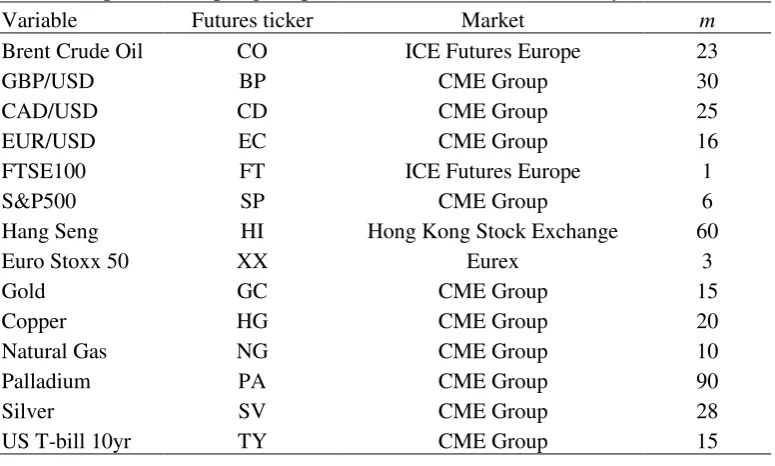
In this study we use tick by tick transaction data of the front-month futures contracts for the following series: Brent Crude Oil (ICE Futures Europe), GBP/USD (CME Group), CAD/USD (CME Group), EUR/USD (CME Group), FTSE100 (ICE Futures Europe), S&P500 (CME Group), Hang Seng (Hong Kong Stock Exchange), Euro Stoxx 50 (Eurex), Gold (CME Group), Copper (CME Group), Natural Gas (CME Group), Palladium (CME Group), Silver (CME Group) and the US 10yr T-bills (CME Group). All data are obtained from Tick Data. We use an additional US macroeconomic volatility indicator which is available in daily frequency, namely the Economic Policy Uncertainty (EPU)5 Index by Baker et al. (2013). The period of our
5
8 study spans from August 1, 2003 to August 5, 2015 and it is dictated by the availability of intraday data for the Brent Crude oil futures contracts.
The choice of variables is justified by the fact that there is a growing literature that confirms the cross-market transmission effects (either of returns or volatilities) between oil and four main asset classes (i.e., Stocks, Forex, Commodities and Macro)6. Given these interactions, we posit that the volatilities of these four asset classes contain important information for the future movements of the oil price volatility. This is related to Ross (1989) who maintains that volatilities are synonymous to the information flow and thus the cross-market transmission effects are synonymous to cross-market information flows or “information channels”.
We consider some specific variables among the four asset classes, largely because they are some of the most tradable futures contracts globally7, but also due to the following reasons.
Specifically, for the stock market indices we choose the key US, EU and Asian indices as (i) their combined trading spans across a full day (24-hours) and (ii) they represent the stock market indices of the largest economies in the world. However, we also include the FTSE100 index futures, given that we forecast the Brent crude oil volatility.
As far as the foreign exchange variables are concerned, we maintain that the EUR/USD is the main currency that exercises an impact on oil fluctuations, while the use of the GBP/USD futures is incontestable, given that it is related to the Brent crude oil. Finally, the choice of the CAD/USD is motivated by Chen et al. (2010) who maintain that currencies of commodity exporters contain important information for the future movements of commodity prices.
Lastly, as macroeconomic indicators we use the US 10yr T-bill futures and the US EPU, as recent studies have shown that oil price volatility is responsive to change in the economic conditions (see, for instance, Antonakakis et al., 2014). We treat both the US 10yr T-bill and the US EPU as variables that approximate global economic developments, given the importance of the US in the global economy.
6
See, inter alia, Aloui and Jammazi (2009), Sari et al. (2010), Arouri et al. (2011), Aloui et al. (2013),
Souček and Todorova (2013, 2014), Mensi et al. (2014), Antonakakis et al. (2014), Sadorsky (2014), Phan et al. (2015), IEA (2015), Ferraro et al. (2015).
7
9 Important milestones for the construction of the intra-day time series are the following:
(i) Trading day: In our paper we define as trading day the period between 21:01 GMT the night before until 21:00 GMT that evening. This particular definition of the trading day is motivated by Andersen et al. (2001, 2003, 2007).
(ii) Holidays: We exclude several fixed and moving holidays from our series, such as Christmas, Martin Luther King day, Washington’s Birthday, Good Friday, Easter Monday, Memorial day, July 4th, Labour day and Thanksgiving and the day after. (iii) Non-trading hours: We remove any trading that takes place between Friday 21:01 GMT until Sunday 21:00 GMT.
(iv) Brent Crude Oil 2-hours Sunday trading session: We use two approaches for the additional 2-hour trading session that occurs in the Brent Crude Oil futures on Sundays. The first approach is to disregard these observations, whereas the second approach is to incorporate these observations to the Monday’s trading day. The results of our forecasting exercise are not affected by the choice of the approach. Given the indifference in the results, we have decided to follow the second approach as it is more instructive to consider all available information in the construction of the realized volatility measure.
(v) Calendar or business-time sampling: We choose the calendar sampling as it is most commonly used in the literature and thus, allows for comparability of the results. Furthermore, as Sévi (2014) explains, the use of business-time sampling is not recommended as its asymptotic properties are less well-known.
(vi) Common sample: Finally, to arrive to a common sample across all series, we have considered the trading days when the Brent Crude Oil is traded8.
After the aforementioned considerations, our final sample consists of 𝑇 =
3028 trading days.
4. Realized volatility
According to Andersen and Bollerslev (1998) the daily realized volatility is estimated to be the sum of squared intra-day returns, as shown in eq.1:
𝐷𝑅𝑉𝑡(𝜏) = √∑ (𝑙𝑜𝑔𝑃𝑡𝑗− 𝑙𝑜𝑔𝑃𝑡𝑗−1)
2 𝜏
𝑗=1 , (1)
8
10 where 𝑃𝑡𝑗 are the observed prices of the asset at trading day t, and τ are the equidistant intraday time intervals.
The realized volatility converges to the integrated volatility as the sampling frequency (m) goes to zero and the number of time intervals (τ) approaches infinity. Nevertheless, more noise is added to the estimated volatility when the sampling frequency converges on zero, due to microstructure frictions. Thus, there is a trade-off between the bias that is inserted in the realized volatility measure and its accuracy. Andersen et al. (2006) suggested the construction of the volatility signature plot, which depicts the average realized volatility against the sampling frequency. Based on the volatility signature plot, the optimal sampling frequency is the one where the autocovariance bias is minimum. In order to identify the point where the realized volatility appears to stabilise, we decompose the inter-day variance (𝑙𝑜𝑔𝑃𝑡−
𝑙𝑜𝑔𝑃𝑡−1)2 into the intra-day variance (𝐷𝑅𝑉𝑡(𝜏)) 2
and the intra-day autocovariance
(∑𝑗=1𝜏−1∑𝜏𝑖=𝑗+1(𝑙𝑜𝑔𝑃𝑡𝑖 − 𝑙𝑜𝑔𝑃𝑡𝑖−1) (𝑙𝑜𝑔𝑃𝑡𝑖−𝑗− 𝑙𝑜𝑔𝑃𝑡𝑖−𝑗−1)), as in eq.2:
(𝑙𝑜𝑔𝑃𝑡− 𝑙𝑜𝑔𝑃𝑡−1)2 = (𝐷𝑅𝑉𝑡(𝜏))
2
+
2 ∑𝑗=1𝜏−1∑𝜏𝑖=𝑗+1(𝑙𝑜𝑔𝑃𝑡𝑖 − 𝑙𝑜𝑔𝑃𝑡𝑖−1) (𝑙𝑜𝑔𝑃𝑡𝑖−𝑗− 𝑙𝑜𝑔𝑃𝑡𝑖−𝑗−1).
(2)
The intra-day autocovariance represents the bias that is inserted in the realized volatility measure, with 𝐸 ((𝑙𝑜𝑔𝑃𝑡𝑖− 𝑙𝑜𝑔𝑃𝑡𝑖−1) (𝑙𝑜𝑔𝑃𝑡𝑖−𝑗− 𝑙𝑜𝑔𝑃𝑡𝑖−𝑗−1)) = 0, for
𝑗 ≠ 0. Thus, the optimal sampling frequency (m) is the highest frequency that
minimises the autocovariance bias. Table 1 shows the optimal sampling frequencies for our series.
[TABLE 1 HERE]
11 markets are closed and thus, they proposed to adjust the intra-day volatility with the close-to-open inter-day volatility, as shown in eq.3:
𝐷𝑅𝑉(𝐻𝐿),𝑡(𝜏) = √𝜔1(𝑙𝑜𝑔𝑃𝑡1 − 𝑙𝑜𝑔𝑃𝑡−1𝜏)
2
+ 𝜔2∑ (𝑙𝑜𝑔𝑃𝑡𝑗 − 𝑙𝑜𝑔𝑃𝑡𝑗−1)
2 𝜏
𝑗=2
, (3)
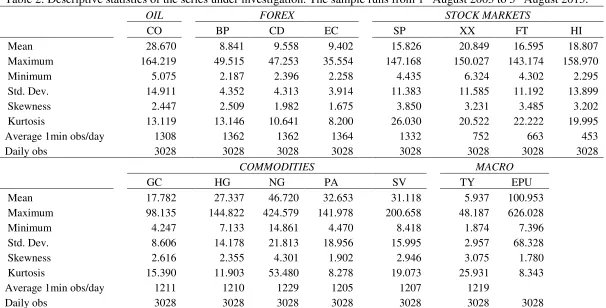
where the weights 𝜔1 and 𝜔2 are such that minimise the difference between the realized volatility and the integrated volatility, i.e. minimise the variance of the realized volatility, min 𝑉 (𝐷𝑅𝑉𝑡,(𝐻𝐿)(𝜏) ). In this paper we are in line with Hansen and Lunde (2005). Table 2 presents the descriptive statistics of our annualised realized volatility series 𝑅𝑉(𝐻𝐿),𝑡(𝜏) :
𝑅𝑉(𝐻𝐿),𝑡(𝜏) = √252 × 𝐷𝑅𝑉(𝐻𝐿),𝑡(𝜏) , (4) for all variables and Figure 1 portrays their plots over the sample period.
[TABLE 2 HERE] [FIGURE 1 HERE]
From Table 2 we notice that EPU has the highest average value and that it is very volatile, given its maximum, minimum and standard deviation values. From the realized volatilities, it is natural gas (NG) that exhibits the highest average volatility, followed by palladium (PA), silver (SV) and oil (CO). On the contrary, the lowest average volatilities are observed in T-bills (TY) and the three exchange rate volatilities (BP, CD and EC). It is also evident that none of the series under consideration are normally distributed, as they exhibit excess kurtosis and positive skewness. Another interesting point is the average number of 1min observations that each series has, with the Eurostoxx 50 (XX), FTSE100 (FT) and Hang Seng (HI) showing the lowest figures, due to the shorter trading sessions that these markets have. The unit root test results support the hypothesis of stationary realized volatilities.
12
5. Econometric specifications
5.1. Naïve models
We consider two naïve models, namely a simple Random Walk (RW) without a drift and an Autoregressive model of order 1, or AR(1), as shown in eqs. 5 and 6, respectively:
𝑙𝑜𝑔 (𝑅𝑉(𝐻𝐿),𝑂𝐼𝐿,𝑡(𝜏) ) = 𝑙𝑜𝑔 (𝑅𝑉(𝐻𝐿),𝑂𝐼𝐿,𝑡−1(𝜏) ) + 𝜀𝑡, (5)
𝑙𝑜𝑔 (𝑅𝑉(𝐻𝐿),𝑂𝐼𝐿,𝑡(𝜏) ) = 𝜑0(𝑡)(1 − 𝜑1(𝑡)) + 𝜑1(𝑡)𝑙𝑜𝑔 (𝑅𝑉(𝐻𝐿),𝑂𝐼𝐿,𝑡−1(𝜏) ) + 𝜀𝑡, (6)
where 𝑅𝑉(𝐻𝐿),𝑂𝐼𝐿,𝑡(𝜏) is the annualised realized volatility of the Brent crude oil at time t,
𝜑0(𝑡), 𝜑1(𝑡) are coefficients to be estimated and 𝜀𝑡 is a white noise.
5.2. HAR-RV model
We employ the HAR model by Corsi (2009), which is recently implemented in Haugom et al. (2014), Sévi (2014) and Prokopczuk et al. (2015)9. Eq. 7 presents the HAR-RV model:
𝑙𝑜𝑔(𝑅𝑉(𝐻𝐿),𝑂𝐼𝐿,𝑡(𝜏) ) =
𝑤0(𝑡)+ 𝑤1(𝑡)𝑙𝑜𝑔 (𝑅𝑉(𝐻𝐿),𝑂𝐼𝐿,𝑡−1(𝜏) ) + 𝑤2(𝑡)(5−1∑ 𝑙𝑜𝑔 (𝑅𝑉
(𝐻𝐿),𝑂𝐼𝐿,𝑡−𝑘(𝜏) ) 5
𝑘=1 ) +
𝑤3(𝑡)(22−1∑ 𝑙𝑜𝑔 (𝑅𝑉
(𝐻𝐿),𝑂𝐼𝐿,𝑡−𝑘(𝜏) ) 22
𝑘=1 ) + 𝜀𝑡,
(7)
where 𝑤0(𝑡), 𝑤1(𝑡), 𝑤2(𝑡), 𝑤3(𝑡) are parameters to be estimated. The HAR-RV model relates the current trading day’s realized volatility of the Brent crude oil to the daily, weekly and monthly realized volatilities of the same asset.
5.3. HAR-RV-X model
We augment the simple HAR-RV model to embody exogenous variables, as discussed in Section 2. The HAR-RV-X model is shown in the following equation:
𝑙𝑜𝑔 (𝑅𝑉(𝐻𝐿),𝑂𝐼𝐿,𝑡(𝜏) ) =
𝑤0(𝑡)+ 𝑤1(𝑡)𝑙𝑜𝑔 (𝑅𝑉(𝐻𝐿),𝑂𝐼𝐿,𝑡−1(𝜏) ) + 𝑤2(𝑡)(5−1∑ 𝑙𝑜𝑔 (𝑅𝑉
(𝐻𝐿),𝑂𝐼𝐿,𝑡−𝑘(𝜏) ) 5
𝑘=1 ) +
𝑤3(𝑡)(22−1∑ 𝑙𝑜𝑔 (𝑅𝑉
(𝐻𝐿),𝑂𝐼𝐿,𝑡−𝑘(𝜏) ) 22
𝑘=1 ) + 𝑤(𝑎),4(𝑡) 𝑙𝑜𝑔 (𝑅𝑉(𝐻𝐿),𝑋(𝜏) (𝑎),𝑡−1) +
(8)
9
13
𝑤(𝑎),5(𝑡) (5−1∑ 𝑙𝑜𝑔 (𝑅𝑉
(𝐻𝐿),𝑋(𝑎),𝑡−𝑘
(𝜏) )
5
𝑘=1 ) +
𝑤(𝑎),6(𝑡) (22−1∑ 𝑙𝑜𝑔 (𝑅𝑉
(𝐻𝐿),𝑋(𝑎),𝑡−𝑘
(𝜏) )
22
𝑘=1 ) + 𝜀𝑡,
where 𝑋(𝑎) denotes each of the fourteen (14) alternative exogenous realized volatilities that are used in this paper.
5.4. HAR-RV-Asset Class, HAR-RV-Combined and HAR-RV-Average models
In order to reveal the predictive information from all the asset volatilities within an asset class without imposing selection and look-ahead biases, we employ the Principal Component Analysis (PCA). In general the techniques for data dimensionality reduction have been successfully applied in now-casting macroeconomic variables (see, for instance, Giannone et al., 2008; Stock and Watson, 2002, among others). PCA enables us to reduce the dimensionality of the existing dataset so that we can reveal the predictive information of asset volatilities, within a single asset class, without losing important information. Hence, most of the available information per asset class in exploited, without imposing selection and look-ahead biases.
More specifically, we construct the HAR-RV-STOCKS, HAR-RV-FOREX, HAR-RV-COMMODITIES and HAR-RV-MACRO models. For each asset class, we use the volatilities that belong to this asset class. E.g. for the HAR-RV-STOCKS we use the volatilities of the four stock market indices to estimate the principal components. For g denoting the number of asset volatilities within the class, the HAR-RV-Asset Class model is illustrated in the following framework:
[
𝑅𝑉(𝐻𝐿),𝑋(𝜏) (1),𝑡 ⋮ 𝑅𝑉(𝐻𝐿),𝑋(𝜏) (𝑔),𝑡
] = 𝜦(𝑔)[
𝑅𝑉(𝑃𝐶𝐴),𝑋(𝜏) (1),𝑡 ⋮ 𝑅𝑉(𝑃𝐶𝐴),𝑋(𝜏) (𝑔),𝑡
] + 𝒆𝑡(𝑔), (9)
𝑙𝑜𝑔 (𝑅𝑉(𝐻𝐿),𝑂𝐼𝐿,𝑡(𝜏) ) =
𝑤0(𝑡)+ 𝑤1(𝑡)𝑙𝑜𝑔 (𝑅𝑉(𝐻𝐿),𝑂𝐼𝐿,𝑡−1(𝜏) ) + 𝑤2(𝑡)(5−1∑ 𝑙𝑜𝑔 (𝑅𝑉
(𝐻𝐿),𝑂𝐼𝐿,𝑡−𝑘(𝜏) ) 5
𝑘=1 ) +
𝑤3(𝑡)(22−1∑ 𝑙𝑜𝑔 (𝑅𝑉
(𝐻𝐿),𝑂𝐼𝐿,𝑡−𝑘(𝜏) ) 22
𝑘=1 ) + 𝑤(𝑎),4(𝑡) 𝑙𝑜𝑔 (𝑅𝑉(𝑃𝐶𝐴),𝑋(𝑎),𝑡−1
(𝜏) ) +
𝑤(𝑎),5(𝑡) (5−1∑ 𝑙𝑜𝑔 (𝑅𝑉
(𝑃𝐶𝐴),𝑋(𝑎),𝑡−𝑘
(𝜏) )
5
𝑘=1 ) +
14
𝑤(𝑎),6(𝑡) (22−1∑ 𝑙𝑜𝑔 (𝑅𝑉
(𝑃𝐶𝐴),𝑋(𝑎),𝑡−𝑘
(𝜏) )
22
𝑘=1 ) + 𝜀𝑡,
where 𝜦(𝑔) is the matrix of factor loadings, [
𝑅𝑉(𝑃𝐶𝐴),𝑋(𝜏) (1),𝑡 ⋮ 𝑅𝑉(𝑃𝐶𝐴),𝑋(𝜏) (𝑔),𝑡
] is the vector with the
common factors, and 𝒆𝑡(𝑔) is the vector of the idiosyncratic component. The 𝑋(𝑎) denotes the common factors that are incorporated in the HAR model for each asset class. The HAR model can be extended to accommodate up to g principal components.
Similarly, we construct the HAR-RV-COMBINED model, which includes the principal components from all 14 asset volatilities, so to capture simultaneously the various “information channels” that could enhance the oil price volatility predictions.
Finally, we also consider the HAR-RV-AVERAGE, which produces the average forecasts from the four HAR-RV-Asset Class models.
5.5. Forecasting realized volatility
Equations 7 - 10 are estimated in the natural logarithms of the realized volatilities. However, we are interested in forecasting the realized volatility, which is the variable of interest for traders, portfolio managers and policy makers. Thus, in our forecasts we concentrate on the estimator of the 𝑅𝑉(𝐻𝐿),𝑂𝐼𝐿,𝑡(𝜏) , which is the
𝑒𝑥𝑝 (𝑙𝑜𝑔 (𝑅𝑉(𝐻𝐿),𝑂𝐼𝐿,𝑡(𝜏) ) + 1 2⁄ 𝜎̂𝜀2). The HAR-RV 1-day-ahead forecast is as follows:
𝑅𝑉(𝐻𝐿),𝑂𝐼𝐿,𝑡+1|𝑡(𝜏) = 𝑒𝑥𝑝 (𝑤̂0(𝑡)+ 𝑤̂1(𝑡)𝑙𝑜𝑔(𝑅𝑉(𝐻𝐿),𝑂𝐼𝐿,𝑡(𝜏) )
+ 𝑤̂2(𝑡)(5−1∑ 𝑙𝑜𝑔(𝑅𝑉
(𝐻𝐿),𝑂𝐼𝐿,𝑡−𝑘+1(𝜏) ) 5
𝑘=1
)
+ 𝑤̂3(𝑡)(22−1∑ 𝑙𝑜𝑔(𝑅𝑉
(𝐻𝐿),𝑂𝐼𝐿,𝑡−𝑘+1(𝜏) ) 22
𝑘=1 ) + 1 2
⁄ 𝜎̂𝜀2)
(11)
15
𝑅𝑉(𝐻𝐿),𝑂𝐼𝐿,𝑡+1|𝑡(𝜏) = 𝑒𝑥𝑝 (𝑤̂0(𝑡)+ 𝑤̂1(𝑡)𝑙𝑜𝑔 (𝑅𝑉(𝐻𝐿),𝑂𝐼𝐿,𝑡(𝜏) )
+ 𝑤̂2(𝑡)(5−1∑ 𝑙𝑜𝑔 (𝑅𝑉
(𝐻𝐿),𝑂𝐼𝐿,𝑡−𝑘+1(𝜏) ) 5
𝑘=1
)
+ 𝑤̂3(𝑡)(22−1∑ 𝑙𝑜𝑔 (𝑅𝑉
(𝐻𝐿),𝑂𝐼𝐿,𝑡−𝑘+1(𝜏) ) 22
𝑘=1
)
+ 𝑤̂(𝑎),4(𝑡) 𝑙𝑜𝑔 (𝑅𝑉(𝐻𝐿),𝑋(𝜏) (𝑎),𝑡)
+ 𝑤̂(𝑎),5(𝑡) (5−1∑ 𝑙𝑜𝑔 (𝑅𝑉
(𝐻𝐿),𝑋(𝑎),𝑡−𝑘+1
(𝜏) )
5
𝑘=1
)
+ 𝑤̂(𝑎),6(𝑡) (22−1∑ 𝑙𝑜𝑔 (𝑅𝑉
(𝐻𝐿),𝑋(𝑎),𝑡−𝑘+1
(𝜏) )
22
𝑘=1 ) + 1 2
⁄ 𝜎̂𝜀2)
(12)
The s-days-ahead forecasts (𝑠 = 2, … , 66 𝑑𝑎𝑦𝑠) are estimated in a similar fashion. More specifically, the s-days-ahead forecast of the HAR-RV model, for horizon
(𝑠 ≥ 2)
𝑅𝑉(𝐻𝐿),𝑂𝐼𝐿,𝑡+𝑠|𝑡(𝜏) =
𝑒𝑥𝑝 (𝑤̂0(𝑡)+ 𝑤̂1(𝑡)𝑙𝑜𝑔 (𝑅𝑉(𝐻𝐿),𝑂𝐼𝐿,𝑡+𝑠−1|𝑡(𝜏) ) +
𝑤̂2(𝑡)(𝑠−1∑ 𝑙𝑜𝑔 (𝑅𝑉
(𝐻𝐿),𝑂𝐼𝐿,𝑡−𝑘+𝑠|𝑡(𝜏) ) 𝑠
𝑘=1 +
(5 − 𝑠)−1∑ 𝑙𝑜𝑔(𝑅𝑉
(𝐻𝐿),𝑂𝐼𝐿,𝑡−𝑘+𝑠(𝜏) ) 5
𝑘=𝑠+1 ) +
𝑤̂3(𝑡)(𝑠−1∑ 𝑙𝑜𝑔 (𝑅𝑉
(𝐻𝐿),𝑂𝐼𝐿,𝑡−𝑘+𝑠|𝑡(𝜏) ) 𝑠
𝑘=1 +
(22 − 𝑠)−1∑ 𝑙𝑜𝑔(𝑅𝑉
(𝐻𝐿),𝑂𝐼𝐿,𝑡−𝑘+𝑠(𝜏) ) 22
𝑘=𝑠+1 ) + 1 2⁄ 𝜎̂𝜀2)
(13)
Finally, the s-days-ahead forecast of the HAR-RV-X models, for horizon (𝑠 ≥ 2)
𝑅𝑉(𝐻𝐿),𝑂𝐼𝐿,𝑡+𝑠|𝑡(𝜏) =
𝑒𝑥𝑝 (𝑤̂0(𝑡)+ 𝑤̂1(𝑡)𝑙𝑜𝑔 (𝑅𝑉(𝐻𝐿),𝑂𝐼𝐿,𝑡+𝑠−1|𝑡(𝜏) ) +
𝑤̂2(𝑡)(𝑠−1∑ 𝑙𝑜𝑔 (𝑅𝑉
(𝐻𝐿),𝑂𝐼𝐿,𝑡−𝑘+𝑠|𝑡(𝜏) ) 𝑠
𝑘=1 +
(5 − 𝑠)−1∑ 𝑙𝑜𝑔(𝑅𝑉
(𝐻𝐿),𝑂𝐼𝐿,𝑡−𝑘+𝑠(𝜏) ) 5
𝑘=𝑠+1 ) +
16
𝑤̂3(𝑡)(𝑠−1∑ 𝑙𝑜𝑔 (𝑅𝑉
(𝐻𝐿),𝑂𝐼𝐿,𝑡−𝑘+𝑠|𝑡(𝜏) ) 𝑠
𝑘=1 +
(22 − 𝑠)−1∑ 𝑙𝑜𝑔(𝑅𝑉
(𝐻𝐿),𝑂𝐼𝐿,𝑡−𝑘+𝑠(𝜏) ) 22
𝑘=𝑠+1 ) + 𝑤̂(𝑎),4(𝑡) 𝑙𝑜𝑔 (𝑅𝑉(𝐻𝐿),𝑋(𝑎),𝑡−𝑘+𝑠|𝑡
(𝜏) ) +
𝑤̂(𝑎),5(𝑡) (𝑠−1∑ 𝑙𝑜𝑔 (𝑅𝑉
(𝐻𝐿),𝑋(𝑎),𝑡−𝑘+𝑠|𝑡
(𝜏) )
𝑠
𝑘=1 +
(5 − 𝑠)−1∑ 𝑙𝑜𝑔 (𝑅𝑉
(𝐻𝐿),𝑋(𝑎),𝑡−𝑘+𝑠
(𝜏) )
5
𝑘=𝑠+1 ) +
𝑤̂(𝑎),6(𝑡) (𝑠−1∑ 𝑙𝑜𝑔 (𝑅𝑉
(𝐻𝐿),𝑋(𝑎),𝑡−𝑘+𝑠|𝑡
(𝜏) ) +
𝑠 𝑘=1
(22 − 𝑠)−1∑ 𝑙𝑜𝑔 (𝑅𝑉
(𝐻𝐿),𝑋(𝑎),𝑡−𝑘+𝑠
(𝜏) )
22
𝑘=𝑠+1 ) + 1 2⁄ 𝜎̂𝜀2)
It is important, though, to explain here how we proceed with the out-of-sample forecasts of 1-day ahead to 66-days ahead, as far as the HAR-RV and HAR-RV-X models are concerned. For the 1-day ahead forecast of the Brent Crude oil, the models use data that belong to the information set at time t and thus, they are known to the forecaster at the time of the forecasting exercise. Nevertheless, from the 2-days ahead forecasts onwards (i.e. 𝑡 + 2, … , 𝑡 + 66), the forecast of the HAR-RV-X models of eq. (8), as well as, the HAR-RV-ASSET CLASS and HAR-RV-COMBINED models of eq. (10), requires the use of future data that do not belong to the information set at time t. For example, for the 𝑡 + 2 forecast we need to know the 𝑡 + 1 volatility values of all variables. As far as the Brent Crude oil volatility is concerned, there is no problem as the model uses the 1-day ahead forecast, i.e. at 𝑡 + 1. Turning to the exogenous variables, there are three possible choices to overcome the issue of using future data that do not belong to the information set at time t.
The first choice is to assume a zero value from 𝑡 + 1 onwards for the volatilities of the exogenous variable(s), since the information is not available at the time of the forecast.
The second choice is to assume that at time 𝑡 + 1 onwards the volatility of the exogenous variable remains constant, i.e. 𝐸 (𝑅𝑉(𝐻𝐿),𝑋
(𝑎),𝑡+1
(𝜏) ) = 𝑅𝑉
(𝐻𝐿),𝑋(𝑎),𝑡
(𝜏) . The
concept that the best forecast of the next days' volatility value is today's value (plus a random component) is referred to as the random walk and it is based on the Efficient Market Hypothesis.
17 forecasts of the Brent crude oil volatility (which are not available at time t), are taken from the forecasted values of these exogenous volatilities.
Between the first two alternatives, the latter is clearly preferred on the grounds that it is closely related to the finance literature and it is easy to implement. To proceed with the second choice, though, we would need to confirm that the RW generates the most accurate forecasts for the exogenous variables and thus to confirm the Efficient Market Hypothesis. To do so, we forecast each of exogenous variables using both a RW model and the HAR-RV model of eq. (7). Our results (not shown here for brevity but they are available upon request) reveal that the HAR-RV model is able to outperform the RW for each of the exogenous variables. Thus, we reject the second choice and we proceed with the Brent Crude oil forecasts based on the third choice. The third choice is shown in eq. (14), where we denote the information of the previous week’s and previous month’s exogenous variables as
(𝑠−1∑ 𝑙𝑜𝑔 (𝑅𝑉
(𝐻𝐿),𝑋(𝑎),𝑡−𝑘+𝑠|𝑡
(𝜏) )
𝑠
𝑘=1 + (5 − 𝑠)−1∑ 𝑙𝑜𝑔 (𝑅𝑉(𝐻𝐿),𝑋(𝑎),𝑡−𝑘+𝑠
(𝜏) )
5
𝑘=𝑠+1 ) and
(𝑠−1∑ 𝑙𝑜𝑔 (𝑅𝑉
(𝐻𝐿),𝑋(𝑎),𝑡−𝑘+𝑠|𝑡
(𝜏) ) + (22 − 𝑠)−1∑ 𝑙𝑜𝑔 (𝑅𝑉
(𝐻𝐿),𝑋(𝑎),𝑡−𝑘+𝑠
(𝜏) )
22 𝑘=𝑠+1 𝑠
𝑘=1 ),
respectively. The first term represents the information from the forecasted exogenous variables, while the second term indicates the information from the constructed exogenous variables10.
This is an important innovation in our approach. The existing literature either ignores this particular procedure (hence, the stated forecasting accuracies can be put into question) or fails to explain it.
6. Forecast evaluation
The initial sample period is 𝑇̃ = 1000 days and we use the remaining
𝑇̆ = 2028 for our out-of-sample forecasting period. The 𝑇̃ = 1000 is justified by the
fact that (i) we require a large sample size for the estimation of the models and (ii) we need our initial sample to stop before the GFC of 2007-08. This allows us to include the recession period in our out-of-sample period. For the first out-of-sample forecasts for 1-day to 66-days ahead, we use the initial sample period 𝑇̃ = 1000. For each
10
18 subsequent forecast, we use a rolling window approach with fixed length of 1000 days. Engle et al. (1993) and Angelidis et al. (2004) maintain that the use of restricted samples is capable of capturing changes in the market activity more accurately.
6.1 Evaluation functions
The forecasting accuracy of the models illustrated in Section 5 is initially evaluated using two well established evaluation functions, namely the Mean Squared Predicted Error (MSE) and the Mean Absolute Predicted Error (MAE):
𝑀𝑆𝐸(𝑠) = 𝑇−1∑ (𝑅𝑉
(𝐻𝐿),𝑂𝐼𝐿,𝑡+𝑠|𝑡(𝜏) − 𝑅𝑉(𝐻𝐿),𝑂𝐼𝐿,𝑡+𝑠(𝜏) ) 2 𝑇
𝑡=1 , (15)
and
𝑀𝐴𝐸(𝑠) = 𝑇−1∑ |𝑅𝑉
(𝐻𝐿),𝑂𝐼𝐿,𝑡+𝑠|𝑡(𝜏) − 𝑅𝑉(𝐻𝐿),𝑂𝐼𝐿,𝑡+𝑠(𝜏) | 𝑇
𝑡=1 , (16)
where 𝑅𝑉(𝐻𝐿),𝑂𝐼𝐿,𝑡+𝑠|𝑡(𝜏) is the s-days-ahead oil realized volatility forecast, whereas
𝑅𝑉(𝐻𝐿),𝑂𝐼𝐿,𝑡+𝑠(𝜏) is the Brent Crude oil realized volatility at time t+s.
6.2 Model Confidence Set
We further employ the newly established Model Confidence Set (MCS) procedure by Hansen et al. (2011), which identifies the set of the best models, as these are defined in terms of a specific loss function, without an a priori choice of a benchmark model11. In our case, the two loss functions are the MSE and MAE12.
The MCS explores the predictive ability of an initial set of 𝑀0 models and investigates, at a predefined level of significance, which group of models survive an elimination algorithm. Let us define as 𝛹𝑛,𝑡 the evaluation function of model 𝑛 at day t, and 𝑑𝑛,𝑛∗,𝑡 = 𝛹𝑛,𝑡− 𝛹𝑛∗,𝑡 as the evaluation differential for 𝑛, 𝑛∗ ∈
𝑀0. For example, the evaluation function may be the Mean Squared Error, so
𝛹𝑛,𝑡≡ (𝑅𝑉(𝐻𝐿),𝑂𝐼𝐿,𝑡+𝑠|𝑡(𝜏) − 𝑅𝑉(𝐻𝐿),𝑂𝐼𝐿,𝑡+𝑠(𝜏) )
2
, where 𝑅𝑉(𝐻𝐿),𝑂𝐼𝐿,𝑡+𝑠|𝑡(𝜏) is the s-days-ahead oil realized volatility forecast. The hypotheses that are being tested are:
11
Most papers compare the forecasts from a variety of models against a benchmark model, utilising the Diebold-Mariano test (Diebold and Mariano, 1995), for a pairwise comparison, the Equal Predictive Accuracy test (Clark and West, 2007) for nested models, or the Reality Check for Data Snooping (White, 2000) and the Superior Predictive Ability test (Hansen, 2005) for multiple comparisons. We depart from this standard setup as in our case we have a number of forecasting models that need to be evaluated simultaneously and not against a benchmark model.
12
19
𝐻0,𝑀: 𝐸(𝑑𝑛,𝑛∗,𝑡) = 0, (17)
for 𝑛, 𝑛∗ ∈ 𝑀, 𝑀 𝑀0 against the alternative hypothesis
𝐻1,𝑀: 𝐸(𝑑𝑛,𝑛∗,𝑡) ≠ 0, for some 𝑛, 𝑛∗ ∈ 𝑀. The elimination algorithm based on an
equivalence test and an elimination rule employs the equivalence test for investigating the 𝐻0,𝑀 for 𝑀 𝑀0 and the elimination rule to identify the model 𝑛 to be removed from M in the case that H0,M is rejected.
6.3 Direction-of-Change
We also consider the Direction-of-Change (DoC) as an additional forecasting evaluation technique. The DoC is particularly important for market timing, which is essential for asset allocation and trading strategies. The DoC reports the proportion of forecasts that have correctly predicted the direction (up or down) of the volatility movement. Let us denote as 𝑃𝑛,𝑖(𝑠) a dummy variable that takes the value of 1 for each trading day i that model 𝑛 correctly predicts the direction of volatility movement s trading days ahead, and zero otherwise, i.e.:
𝑃𝑛,𝑖(𝑠) = {
1 𝑖𝑓 𝑅𝑉(𝐻𝐿),𝑂𝐼𝐿,𝑡+𝑠(𝜏) > 𝑅𝑉(𝐻𝐿),𝑂𝐼𝐿,𝑡(𝜏) 𝑎𝑛𝑑 𝑅𝑉(𝐻𝐿),𝑂𝐼𝐿,𝑡+𝑠|𝑡(𝜏) > 𝑅𝑉(𝐻𝐿),𝑂𝐼𝐿,𝑡(𝜏)
1 𝑖𝑓 𝑅𝑉(𝐻𝐿),𝑂𝐼𝐿,𝑡+𝑠(𝜏) < 𝑅𝑉(𝐻𝐿),𝑂𝐼𝐿,𝑡(𝜏) 𝑎𝑛𝑑 𝑅𝑉(𝐻𝐿),𝑂𝐼𝐿,𝑡+𝑠|𝑡(𝜏) < 𝑅𝑉(𝐻𝐿),𝑂𝐼𝐿,𝑡(𝜏)
0 𝑜𝑡ℎ𝑒𝑟𝑤𝑖𝑠𝑒.
(18)
Then, the proportion of forecasted values that have correctly predicted the direction of the volatility movement (𝐷𝑜𝐶𝑝𝑟𝑜𝑝(𝑠) ) is shown in eq. 19:
𝐷𝑜𝐶𝑝𝑟𝑜𝑝(𝑠) =
∑𝑇̌ 𝑃𝑛,𝑖(𝑠)
𝑖=1
𝑇̌ × 100, (19)
where 𝑇̌ is the number of out-of-sample forecasted values. The statistical significance of the directional accuracy is gauged by the Pesaran and Timmermann (2009) test, under the null hypothesis of no directional accuracy.
7. Empirical results
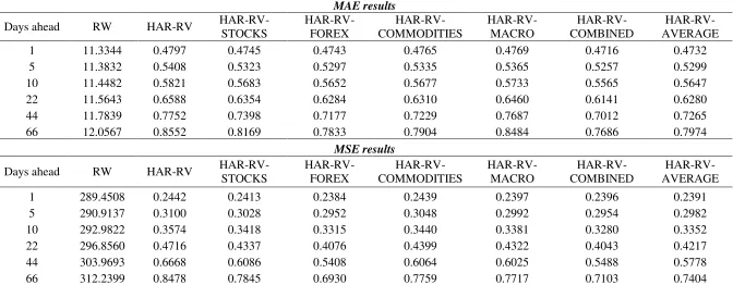
7.1. MAE and MSE
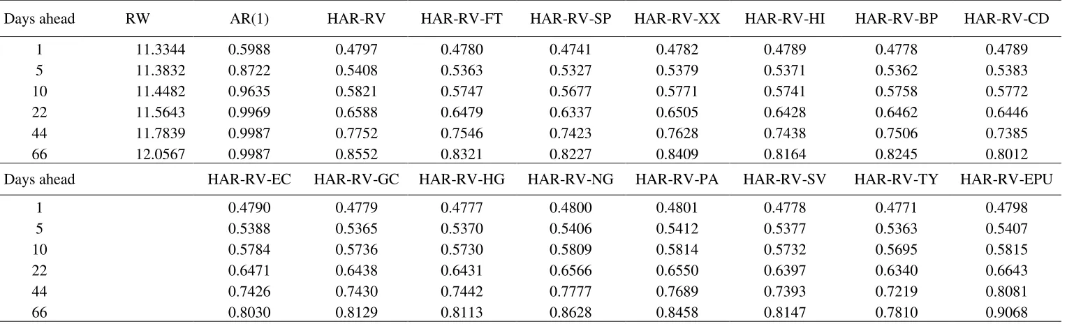
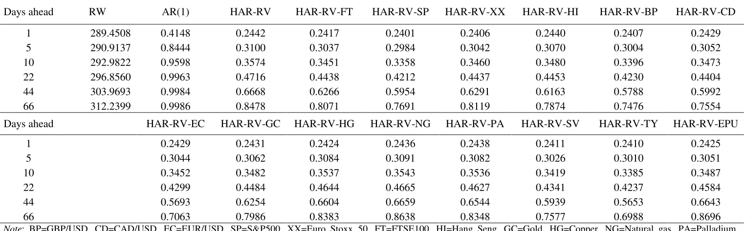
20 Tables 3a, 3b and 4. In the first column we report the value of the loss functions for the RW model, whereas in the remaining columns we report the loss functions’ ratios, relative to the RW model. A score below 1 denotes that the forecasts of the HAR-RV models outperform these of the RW.
[TABLE 3a HERE] [TABLE 3b HERE] [TABLE 4 HERE]
Primarily, it is evident in Tables 3a, 3b and 4 that all HAR-RV models are able to significantly outperform the RW forecasts. In more detail, focusing on Tables 3a and 3b, we show that almost all HAR-RV-X models with a single exogenous volatility are able to generate superior forecasts even when compared to the HAR-RV. This is particularly evident for the HAR-RV-X models with the foreign exchange volatilities and the US T-bill volatility and to a lesser extend for the commodities and stock markets. The only exceptions are the EPU and the Natural Gas volatility, which yield comparable results with the simple HAR-RV model..
More interesting findings, though, are reported in Table 4, which shows the forecasting performance of the RV-Asset Class models, as well as, the HAR-RV-COMBINED and HAR-RV-AVERAGE models. In particular, we find that the HAR-RV-COMBINED model is able to generate significantly improved forecasts not only relatively to the RW, but also to the simple HAR-RV model. This holds true for all forecasting horizons. Even more, the predictive gains from the HAR-RV-COMBINED model relatively to the RW and the simple HAR-RV are higher as the forecasting horizon increases. In greater detail, the HAR-RV-COMBINED is able to reduce the forecasting error, in terms of MAE, by more than 50% (compared to the RW) in short-run horizons and more than 23% in long-run horizons. Equivalently, the HAR-RV-COMBINED model reduces the forecasting error by more than 10% in the long-run horizons, compared to the single HAR-RV. A plausible explanation as to why the HAR-RV-COMBINED is the best performing model lies to the fact that oil price volatility is not influenced by a single asset class throughout the sample period, but rather it is impacted by different asset classes and, thus, different “information channels”. Interestingly enough, the HAR-RV-AVERAGE model does not manage to improve further the forecasting accuracy of the HAR-RV-COMBINED.
21 accurate forecasts. In this paper we provide evidence that the incorporation of different asset classes’ volatilities is capable of generating superior forecasts compared to the HAR-RV model, since they accommodate for the fact that oil volatility is impacted by different “information channels”.
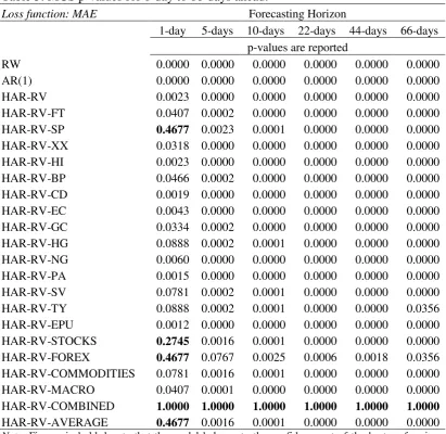
7.2. Model Confidence Set (MCS) procedure
Next, we discuss the results from the MCS procedure, reported in Table 5. Even though the results from Tables 3a, 3b and 4 suggest that the inclusion of the exogenous volatilities significantly improves the forecasting performance of the HAR-RV model, it is vital to assess whether the simple HAR-RV can be included among the best performing models.
[TABLE 5 HERE]
From Table 5 we can make the following observations. First and foremost, the two naïve models and the HAR-RV are never among the best performing models and the same holds for the HAR-RV-X models with the single asset volatility13. We also note that the highest probability is assigned to the HAR-RV-COMBINED model, which is the HAR-RV models that is augmented with the use of multiple exogenous volatility “information channels”. This holds across all horizons. Another interesting finding from Table 5 is the fact that only in the 1-day ahead forecasting horizon, the HAR-RV-STOCKS, HAR-RV-FOREX and HAR-RV-AVERAGE are also included in the set of the best performing models. Overall, the findings presented in Table 5 strengthen the conclusion that the predictive accuracy of the oil price realized volatility increases when we include the exogenous volatilities of multiple asset classes.
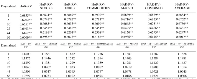
7.3. Direction-of-Change results
The DoC results are shown in Table 6, which reports the proportion of forecasted values that have correctly predicted the direction of volatility movement, as well as the DoC performance of each HAR-RV model against the RW.
[TABLE 6 HERE]
Table 6 shows that all HAR-RV models exhibit statistically significant directional accuracy of the oil volatility movements. Interestingly enough, even
13
22 though the simple HAR-RV model is not included among the best models (as suggested by the MCS test) its ability to predict the direction of change is comparable to that of all HAR-RV-X models. From Table 6 we further notice that all HAR-RV models are able to predict the direction of change at a much higher rate compared to the RW model in all forecasting horizons.
7.4. Summary of findings
Overall, evidence suggests that the use of the exogenous volatilities of different asset classes results in substantial improvement in the forecasting accuracy of Brent Crude oil volatility. More importantly though, we highlight that as we move towards longer-run forecasting horizons, where accurate forecasts are more difficult to make, the predictive gains from the HAR-RV-COMBINED are becoming more prevalent. On the other hand, focusing on the DoC, we maintain that all models are highly accurate in predicting the direction of oil volatility movements. Thus, the combination of the MCS and the DoC results reveals a very important finding which has not been previously discussed in this strand of the literature.
These findings reveal that the simple HAR-RV model would be adequate for the stakeholders interested in the future movement of oil price volatility. Nevertheless, stakeholders who put more emphasis on the accuracy of the forecasts should use the HAR-RV-X models and more specifically, the HAR-X-COMBINED model. Finally, the fact that the HAR-RV-COMBINED outperforms all other models provides support to our claim that different asset classes provide different information to oil price volatility and thus, their combination improves the forecasting accuracy.
8. Robustness and further tests
8.1 Distribution of forecast errors
The first robustness check is related to the distribution of the forecast errors. More specifically, the squared difference and the absolute difference between the oil realized volatility forecast (𝑅𝑉(𝐻𝐿),𝑂𝐼𝐿,𝑡+𝑠|𝑡(𝜏) ) and the realized volatility
23 higher forecasting accuracy, the actual deviation between the model’s predicted volatilities and the actual values may be lower than the reported ones from MSE and MAE. To illustrate this, we first present the distribution of the absolute and squared deviations between the forecasted values from HAR-RV-COMBINED and the actual oil realized volatility (see Figure 2).
[FIGURE 2 HERE]
As evident from Figure 2, the distribution of the deviations is highly skewed, which provides support to our claim that it is instructive to use the median deviations (i.e. the Median Absolute Error – MeAE or the Median Squared Error - MeSE), as they may assess the magnitude of the prediction error more accurately.
From Table 7 and Figure 3 we observe that as the forecasting horizon increases, the magnitude of the prediction errors differs greatly between the mean and the median deviation. For example, the MAE (MSE) for the 1-day ahead forecast is reported to be 5.3457 (69.3662), whereas the MeAE (MeSE) is estimated at 3.6661 (13.4401). Equivalently, for the 66-days ahead, even though the MAE (MSE) reports values of the magnitude of 9.2670 (221.7807), the MeAE (MeSE) are only 5.7089 (32.5920).
[TABLE 7 HERE] [FIGURE 3 HERE]
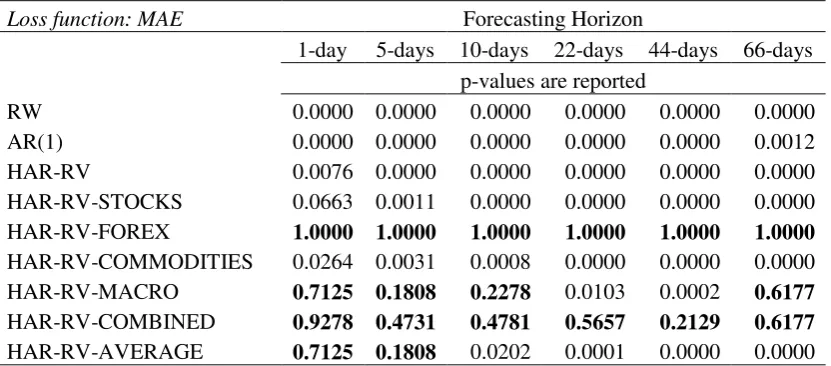
8.2 Predictive accuracy during crisis periods
As a further robustness check we assess the validity of our findings in extreme economic conditions, such as the GFC of 2007-08. We follow the same forecasting evaluation procedure and we evaluate our forecasts only for the period between August, 2007 and June, 2009. For brevity, we only present the results from the MCS procedure and we concentrate only on the ASSET CLASS, HAR-RV-COMBINED and HAR-RV-AVERAGE models (see, Table 8).
[TABLE 8 HERE]
24 Furthermore, we observe that in the short-run horizons, the HAR-RV-MACRO and HAR-RV-AVERAGE models are also among the models with the best predictive accuracy. Overall, the MCS results shown in Table 8 corroborate the findings from Table 5, and it also highlights the fact that during turbulent times, the Forex can also provide important predictive information at all horizons. Overall, we maintain that the evidence provided by the robustness check validates the proposed forecasting strategy plan, as it is effective even under extreme economic conditions.
8.3 Incremental value of the HAR-RV-X models
We shall remind the reader that the MCS test, shown in Section 7.2, provides convincing evidence that the HAR-RV-COMBINED model is always included in the set of the best performing models, whereas the simple HAR-RV model is never included in this set. It is, thus, important to show the incremental value of the incorporation of exogenous volatilities in the HAR-RV model, over time. To do so, we compare the HAR-RV-COMBINED with the HAR-RV model, given that the former is our best performing model, whereas the latter is the best model based on the existing literature.
The cumulative incremental value is estimated by deducting the MAE score of the HAR-RV model from the MAE score of the HAR-RV-COMBINED for the whole out-of-sample forecasting period. Thus, an upward movement of the line suggests that the HAR-RV-COMBINED is having a positive incremental value compared to the HAR-RV. The reverse holds true when the line is moving downwards. For brevity, Figure 4 shows the cumulative incremental value for the 1-day ahead forecasts, based on the MAE loss function.
[FIGURE 4 HERE]
Overall, we find that the incremental value of the use of exogenous asset volatilities is substantial over the forecasting period. More importantly though, we observe that during turbulent periods (such as the GFC of 2007-08 and the oil price collapse in 2014-15) the incremental value of the HAR-RV-COMBINED model is sizeable, as indicated by the steep upward movement of the line.
8.4 Forecast evaluation based on a trading strategy
day-25 trading strategy. Indicatively, for the 1-day ahead forecasts, we assume that a trader assumes a long position in an asset that resembles the performance of the oil realized volatility when the t1forecasted oil price volatility of model n is higher compared to the actual volatility at time
t
. By contrast, if the t1forecasted volatility of modeln is lower compared to the actual volatility at time
t
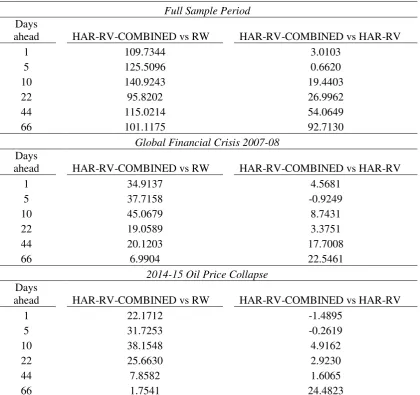
, then the trader assumes a short position. The trading game is constructed in a similar fashion for the remaining forecasting horizons. Volatility portfolio returns are then computed as the average daily returns over the investment horizon, which equals our out-of-sample forecasting period of 𝑇̌=2028 days.The results of the trading strategy are reported in Table 9. It is evident that the HAR-RV-COMBINED provides greater positive returns compared to both the RW and the HAR-RV models. As expected, the cumulative difference in returns is greater between the COMBINED and RW as opposed to the HAR-RV-COMBINED and HAR-RV. Nevertheless, the difference in returns is sizeable in both cases. This holds true even for the crisis periods, such as the GFC of 2007-08 and the oil collapse in 2014-15. Overall, these findings confirm superiority of the HAR-RV-COMBINED model.
[TABLE 9 HERE]
8.5 Forecast evaluation based on option straddles trading profitability metrics
Based on Andrada-Felix et al. (2016), Angelidis and Degiannakis (2008), Engle et al. (1993) and Xekalaki and Degiannakis (2005), we additionally employ an options straddle trading strategy as an additional economic criterion to evaluate the volatility forecasts of different models. In particular, we allow investors to go long (short) in a straddle when the forecasted volatility at time t+s is higher (lower) than the oil realized volatility at the present time t.
26 The expected price of a straddle on a $1 share of the Brent crude oil at the next trading day with 𝑠 days to maturity and $1 exercise price is computed as:
𝑆𝑡+1\𝑡= 2𝑁 (𝑅𝑉̅̅̅̅𝑟𝑓𝑡+𝑠|𝑡𝑡√𝑠 +𝑅𝑉
̅̅̅̅𝑡+𝑠|𝑡√𝑠
2 ) − 2𝑒−𝑟𝑓𝑡𝑠𝑁 (
𝑟𝑓𝑡√𝑠
𝑅𝑉
̅̅̅̅𝑡+𝑠|𝑡−
𝑅𝑉
̅̅̅̅𝑡+𝑠|𝑡√𝑠
2 ) +
𝑒−𝑟𝑓𝑡𝑠− 1,
(20)
whereN
. denotes the cumulative normal distribution function,𝑅𝑉
̅̅̅̅𝑡+𝑠|𝑡 = 1
𝑠−1∑ (
𝑅𝑉(𝐻𝐿),𝑂𝐼𝐿,𝑡+𝑖|𝑡(𝜏)
√252 ) 𝑠
𝑖=1 is the average volatility forecast during the life of
the option, and 𝑟𝑓𝑡is the risk-free interest rate. The daily profit from holding the straddle is: 𝜋𝑡+1= 𝑚𝑎𝑥(𝑒𝑦𝑡+1−𝑒𝑟𝑓𝑡+1, 𝑒𝑟𝑓𝑡+1 − 𝑒𝑦𝑡+1), for 𝑦𝑡 denoting the Brent
crude oil daily log-returns.
We assume the existence of three investors who trade their volatility forecasts. Each investor 𝑖 prices the straddles, 𝑆𝑡+1\𝑡(𝑖) , every trading day according to one of the three volatility forecasting models; i.e. RW, HAR-RV and HAR-RV-COMBINED. A trade between two investors, 𝑖 and 𝑗, is executed at the average of their forecasting prices, yielding to investor 𝑖 a profit of:
𝜋𝑡(𝑖,𝑗) = {𝜋𝑡+1− (𝑆𝑡+1\𝑡
(𝑖) + 𝑆
𝑡+1\𝑡(𝑗) )
(𝑆𝑡+1\𝑡(𝑖) + 𝑆𝑡+1\𝑡(𝑗) ) − 𝜋𝑡+1
if if
𝑆𝑡+1\𝑡(𝑖) > 𝑆𝑡+1\𝑡(𝑗)
𝑆𝑡+1\𝑡(𝑖) < 𝑆𝑡+1\𝑡(𝑗) . (21)
As an economic evaluation criterion, we define the cumulative returns computed as
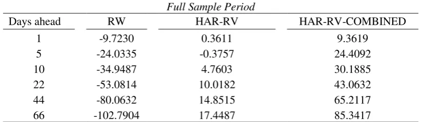
𝜋 = 12∑𝑇̌𝑡=1∑2𝑗=1𝜋𝑡(𝑖,𝑗). Table 10 presents the cumulative returns, for 𝑇̌ trading days,
of investors who pricing their straddles according the RW, HAR-RV and HAR-RV-COMBINED volatility forecasts. The results show that the HAR-RV-HAR-RV-COMBINED is once again superior compared to the other models14.
[TABLE 10 HERE]
8.6 HAR-RV-X models using time-varying correlations
Finally, we repeat the same forecasting strategy replacing the exogenous asset volatilities in the HAR-RV-X models with the time-varying correlations between the volatilities of the Brent crude oil and the 14 remaining assets. We do this in order to
14
For robustness purposes, the straddles trading game has been repeated for i) the exercise price being equal to the exponent of the risk free rate of return and ii) various levels of exercise prices; i.e. 𝑒−3𝑟𝑓𝑡.
27 assess whether we can enhance the predictive accuracy of oil price volatility using a different measure to extract information from the four aforementioned asset classes.
For the estimation of the time-varying correlations we use the multivariate DCC model of Engle (2002). We denote the vector that comprises the log-realized
volatility of the oil price and the other 14 assets as 𝒀𝑡 ≡
[
𝑙𝑜𝑔 (𝑅𝑉(𝐻𝐿),𝑂𝐼𝐿,𝑡(𝜏) )
𝑙𝑜𝑔 (𝑅𝑉(𝐻𝐿),𝑋(𝜏) (1),𝑡)
⋮
𝑙𝑜𝑔 (𝑅𝑉(𝐻𝐿),𝑋(𝜏) (14),𝑡)]
. The
DCC model is estimated in the form:
𝒀𝑡 = 𝑩0+ 𝜺𝑡,
𝜺𝑡 = 𝜢1/2𝜏 𝒛𝑡,
(22) where 𝑩0 is a vector of constants and 𝒛𝑡~𝑁(𝟎, 𝑰). The variance-covariance matrix is decomposed as:
𝑯𝑡 = 𝜮𝑡1/2𝑪𝑡𝜮1/2𝜏 . (23)
The 𝜮1/2𝑡 is a diagonal matrix with the conditional standard deviations along the diagonal defined as GARCH(1,1) processes, whereas the
𝑪𝑡 =
[
1 𝑐𝑜𝑟𝑂𝐼𝐿,𝑋(1),𝑡 ⋯ 𝑐𝑜𝑟𝑂𝐼𝐿,𝑋(14),𝑡 𝑐𝑜𝑟𝑂𝐼𝐿,𝑋(1),𝑡 1 ⋯ 𝑐𝑜𝑟𝑋(1),𝑋(14),𝑡
⋮ 𝑐𝑜𝑟𝑂𝐼𝐿,𝑋(14),𝑡
⋮
𝑐𝑜𝑟𝑋(1),𝑋(14),𝑡
⋱ ⋮
⋯ 1 ]
is the conditional correlations'
matrix15.
Then, we employ eqs. 8, 10, 12 to forecast the oil price realized volatility using the alternative HAR-RV-X models. More specifically, the HAR-RV-X model is modified in the following form:
𝑙𝑜𝑔 (𝑅𝑉(𝐻𝐿),𝑂𝐼𝐿,𝑡(𝜏) ) =
𝑤0(𝑡)+ 𝑤1(𝑡)𝑙𝑜𝑔 (𝑅𝑉(𝐻𝐿),𝑂𝐼𝐿,𝑡−1(𝜏) ) + 𝑤2(𝑡)(5−1∑ 𝑙𝑜𝑔 (𝑅𝑉
(𝐻𝐿),𝑂𝐼𝐿,𝑡−𝑘(𝜏) ) 5
𝑘=1 ) +
𝑤3(𝑡)(22−1∑ 𝑙𝑜𝑔 (𝑅𝑉
(𝐻𝐿),𝑂𝐼𝐿,𝑡−𝑘(𝜏) ) 22
𝑘=1 ) + 𝑤4(𝑡)𝑐𝑜𝑟𝑂𝐼𝐿,𝑋(𝑎),𝑡−1+
𝑤5(𝑡)(5−1∑ 𝑐𝑜𝑟
𝑂𝐼𝐿,𝑋(𝑎),𝑡−𝑘
5
𝑘=1 ) + 𝑤6(𝑡)(22−1∑22𝑘=1𝑐𝑜𝑟𝑂𝐼𝐿,𝑋(𝑎),𝑡−𝑘) + 𝜀𝑡,
(24)
where 𝑋(𝑎) denotes each of the alternative exogenous variables.
15
The matrix of conditional correlations is estimated as 𝑪𝑡= 𝑸𝑡∗−1/2𝑸𝑡𝑸𝑡∗−1/2, where 𝑸𝑡=
(1 − 𝑎 − 𝑏)𝑸̅ +α(𝒛𝑡−1𝒛′𝑡−1) + b𝑸𝑡−1, for 𝑸̅ being the unconditional covariance of the standardized
28 We further repeat the same forecasting strategy using the log-returns’ time
-varying correlations; i.e. the DCC model is estimated for 𝒀𝑡 ≡ [
𝑦𝑂𝐼𝐿,𝑡
𝑦𝑋(1),𝑡
⋮
𝑦𝑋(14),𝑡
], where 𝑦𝑋(𝑎),𝑡
denotes the log-returns of the 𝑋(𝑎) asset. Hence, the the conditional correlations' matrix 𝑪𝑡 contains the conditional correlations between oil log-returns and exogenous variables’ log-returns. For brevity, we only present the ratio of the MAE and MSE between the HAR-RV-X models based on the asset volatilities and the time-varying correlations. The results are shown in Table 11.
[TABLE 11 HERE]
All ratios are below one, which suggests that the HAR-RV-X models based on the asset volatilities are able to provide superior predictive accuracy compared to the alternative HAR-RV-X models, which are based on the time-varying correlations of either volatilities or returns. Indicatively, the 0.8395 MAE ratio, in the 66-days ahead horizon under the HAR-RV-COMBINED column, suggests that the time-varying return correlations provide about 16% lower predictive accuracy compared to the asset volatilities.
9. Conclusion
The aim of this paper is to contribute to the limited but growing literature on oil price realized volatility forecasting. To do so we use tick by tick data of the front-month futures contracts for 14 asset prices. The period of our study spans from August 1, 2003 to August 5, 2015, which provides us with a total of 3028 trading days. Our forecasting horizons range from 1-day to 66-days ahead, given that different stakeholders have different predictive needs.
The current consensus provides evidence that the HAR-RV model outperforms all other competing forecasting models (see, Haugom et al., 2014; Sévi, 2014; Prokopczuk et al., 2015). Our paper builds upon these previous contributions and extends them in multiple ways.
29 (HAR-RV-COMBINED) is the best performing models. Interestingly enough, the Direction of Change suggests that all HAR models are highly accurate in predicting the movements of oil price volatility. Thus, we maintain that HAR-RV-X models should be used by stakeholders who are interested in the accuracy of the forecasts, whereas those interested only in the movement of oil price volatility could be limited to HAR-RV. It is important to note that our findings are robust even when we concentrate only on turbulent economic periods, such as the Global Financial Crisis of 2007-08. Finally, the trading game confirms that the HAR-RV model which is augmented with the use of exogenous volatilities from multiple asset classes offers higher returns compared to both the RW and the simple HAR-RV.
More importantly, the fact that HAR-RV-COMBINED model is the best performing model provides strong support to our argument that there are different “information channels” through which different asset classes could impact oil price volatility and thus, their combination enhances the predictive accuracy of the simple HAR-RV model.
An interesting direction for further research would be the use of our forecasting strategy for the prediction of other assets’ volatilities. Finally, it would also be research-worthy to investigate whether the predictive added-value of the “information channels” featured in this paper would remain qualitatively comparable if we considered alternative measures of volatility, such as the bi-power variation, the median realized variance and the realized semi-variance.
Acknowledgements
The authors acknowledge the support of the European Union's Horizon 2020 research and innovation programme, which has funded them under the Marie Sklodowska-Curie grant agreement No 658494. We also thank Lutz Kilian, Simos Meintanis, Stephen Millard, Nikos Nomikos, Perry Sadorsky, Apostolos Serletis, Lorenzo Trapani and Benoît Sévi for their valuable comments on an earlier version of the paper. Finally, we would also like to thank the participants of the ISEFI 2016 conference, as well as, the participants of the research seminars at the Bank of Greece, Athens University of Economics and Business, Panteion University of Social and Political Sciences and University of Athens.