Numerical and experimental study of flow in a gas turbine chamber

Numerical and experimental study of flow in a gas turbine

chamber.

DAUD, Harbi Ahmed.

Available from Sheffield Hallam University Research Archive (SHURA) at:

http://shura.shu.ac.uk/19535/

This document is the author deposited version. You are advised to consult the publisher's version if you wish to cite from it.

Published version

DAUD, Harbi Ahmed. (2012). Numerical and experimental study of flow in a gas turbine chamber. Doctoral, Sheffield Hallam University (United Kingdom)..

Copyright and re-use policy

See http://shura.shu.ac.uk/information.html

Sheffield

1 0 2 0 7 0 936

1WD

7

ProQuest Number: 10694416

All rights reserved

INFORMATION TO ALL USERS

The quality of this reproduction is dependent upon the quality of the copy submitted.

In the unlikely event that the author did not send a com plete manuscript and there are missing pages, these will be noted. Also, if material had to be removed,

a note will indicate the deletion.

uest

ProQuest 10694416

Published by ProQuest LLC(2017). Copyright of the Dissertation is held by the Author.

All rights reserved.

This work is protected against unauthorized copying under Title 17, United States C ode Microform Edition © ProQuest LLC.

ProQuest LLC.

789 East Eisenhower Parkway P.O. Box 1346

Numerical and Experimental study of

Flow in a Gas Turbine Chamber

Harbi Ahmed Daud

A thesis submitted in partial fulfilment of the requirements of

Sheffield Hallam University

for the degree of Doctor of Philosophy

By the grace o f Allah the almighty, this thesis is dedicated to prophet Mohammed (peace and blessing be upon him), and to the loving memory o f my father Ahmed Daud

Abstract

This thesis examines the cooling performance and the flow on a gas turbine blade. Numerical and experimental methods are described and implemented to assess the influence of film cooling effectiveness. A modem gas turbine blade geometry has been used. The blade is considered as a solid body with the blade cross section from hub to shroud varying with a degree of skewness. Computational Fluid Dynamics (CFD) is employed to assess blade film cooling effectiveness via simulation of the effect of varying blowing ratios (BR=1, 1.5 and 2), varying coolant fluid temperature (Tc=153 K and Tc=287.5 K), various angles of injection (35°,45° and 60°), increasing the number of cooling holes (32 and 42) and increasing the cooling holes diameter (D= 0.5 mm and 1mm). A full three-dimensional finite-volume method has been utilized in this study via the FLUENT 6.3 code with a k-s (RNG) turbulence model.

Results of the CFD models were carefully validated by studying aerodynamic flow and heat transfer in turbine blade film cooling performance. A two-dimensional channel and NACA 0012 airfoil were selected to investigate turbulence effects. The solution accuracy is assessed by carrying out a sensitivity analysis of mesh type and quality effects with enhancement wall treatment and standard wall function effects also addressed for turbulent boundary layers. In this study, four different turbulence models were utilized (S-A, k~e, (RNG), and (SST) k~co). The computations were compared with available Direct Numerical Simulation (DNS) and experimental data. Good correlation was observed when using the RNG turbulence model in comparison with other turbulence models.

Film cooling effectiveness and heat transfer along a flat plate has been analyzed for four different plate materials, namely steel, carbon steel, copper and aluminum, with 30° angle of injection. The cooling holes arrangement was simulated for a hole diameter of

D=1 mm and different sections of the blade showing cooling effectiveness and heat

Acknowledgments

First, I would like to express my sincere gratitude and thanks to ALLAH for the guidance through this work and for all the blessings bestowed upon me. This study would not have been possible without the help of ALLAH.

I would also like to pay special thanks to my supervision team, primarily my director of study Dr. O. Anwar Beg for his continued support, patience and encouragement from 2008 to present, with all aspects of the work.

To my supervisor Dr Qinling Li I am grateful for her guidance and suggestions during this research. Dr Li always provided excellent advice in particular on the CFD simulations.

To my external research adviser, Dr Saud Ghani for his advice and efforts concerning the experimental work and for his excellent support and supervision of wind tunnel experiments in Qatar University in the summer of 2011.

I am truly and deeply indebted to Dr Beg, Dr Li and Dr Ghani and I wish to extend my sincere gratitude to them for giving me this opportunity to conduct research under their supervisions.

I would like to thanks the Government of Iraq, Ministry of higher Education for their generous financial support during my studies at Sheffield Hallam University.

I would like to thanks Sheffield Hallam University and in particular the Materials and Engineering Research Institute (MERI).

I would like also to thank Qatar University and in particular the Mechanical and Industrial Engineering Department for their hospitality and for providing the opportunity to carry out experimental work in gas turbine film cooling under the supervision of Dr. Saud Ghani. I also wish to express my special gratitude to Mr. Yehia ElSaid for his support in setting up the thermal wind tunnel in the power generation lab. Without their help the experimental tests would not had been carried out fruitfully.

I would also like to thank Wolverhampton University and especially Dr. Mark Stanford for his assistance with the fabrication of blade turbine specimens used laser sintering technology.

Preface

The present work in this thesis was performed by PhD student, Harbi A. Daud, between October 2008 and January 2012 in the Materials Engineering and Research Institute (MERI), Sheffield Hallam University.

Numerical simulation of gas turbine flow is an important engineering problem which involves heat transfer, turbulence and film cooling technology in complex geometries. An important objective in the present study is to highlight the significance of validation of CFD simulations achieved with the commercial package FLUENT, with experimental tests, in order to accurately predict aerodynamic flow and heat transfer characteristics for a gas turbine blade.

As a result of this research, a number of journal and conference papers were published and no part of it has been submitted for award at any other College or University.

PhD candidate contributions:

1. Poster presentation for MERI Student seminar day in Sheffield Hallam University,

25th May 2009.

2. Oral presentation (20 minutes) for MERI Student seminar day in Sheffield Hallam

University, 25th May 2010.

3. Refereed Journal article: Daud H. A., Li Q. , Beg O. A. and. AbdulGhani S. A. A.

(20011A)„ Numerical investigations of wall-bounded turbulence. Proc. IMechE Part C- J. Mechanical Engineering Science, 2011. 225, p. 1163-1174.

4. Refereed Conference article: Daud H. A., Li Q ., Beg O. A. and. AbdulGhani S. A.

A.(20011B), Numerical simulation of blowing ratio effects on film cooling on a

gas turbine blade, Computational Methods and Experimental Measurements XV

Conference. 2011: 31st May - 2nd June, New Forest, UK p. 279-292.

5. Refereed Conference article: Daud H. A., Li Q. , Beg O. A. and. AbdulGhani S. A.

A.(2011C), Numerical study of flat plate film cooling effectiveness with

different material properties and hole arrangements, 12th UK National Heat

Transfer Conference, 30/31st August - 1st September 2011, University of Leeds, UK.

6. Oral and poster presentation of engineering sciences conference 1st & 2nd October

(This achieved a 1st prize for Best Poster in Mechanical and Manufacture Engineering).

7. Daud H. A., Li Q., Beg O. A. and. AbdulGhani S. A. A., Numerical Investigation of Film Cooling Effectiveness and Heat Transfer along a Flat Plate, Int. J. o f

Applied Mathematics and Mechanics (IJAMM) 8(17) p.17-33 (2012).

8. Refereed Journal article: Harbi A. Daud, S A.A Abdul Ghani, O. Anwar Beg,

Qinling Li and Mark Stanford, Investigation of gas turbine film cooling using

thermal paint technology, Experiments in Fluids, January (2012). Submitted

Table of Contents Abstract

Acknowledgments Preface Declaration List of Figures

List of Tables Nomenclature Abbreviations

Ctuiptm (9ne JnUaductian 1

1.1 General introduction... 2

1.2 International historical perspective of patents... 3

1.2.1 British efforts... 3

1.2.2 French efforts... 4

1.2.3 German efforts... 4

1.2.4 USA efforts... 5

1.3 Gas turbine cooling method... 7

1.3.1 Convection cooling method... 7

1.3.2 Impingement cooling method... 7

1.3.3 Film cooling method... 8

1.3.4 Transpiration cooling method... 9

1.4 Technology of cooling blades in a gas turbine... 9

1.5 Aim of the research... 11

1.6 Objective of the research... 11

1.7 Motivation of the research... 12

Chapter Juia £it&uitwte {Review 15 2.1 Introduction... 16

2.2 Fluid flow analysis... 16

2.2.1 Wall bounded turbulence... 17

2.2.2 Aerodynamics of gas turbines... 19

2.3 Heat transfer and film cooling studies... 22

2.3.1 Flat and curved plates... 22

2.3.2 Gas turbine film cooling... 27

2.4 Methodology... 34

Chapter 5(vtez Jntmduction ta Compiitatwnal &tuid {Dynamic# ( C3{D) 37 <£ JVumeacal Equation# 3.1 Introduction... 38

3.2 Mathematical model of the fluid flow... 38

3.2.1 Navier-Stokes equation... 38

3.3 Solution procedure... 39

3.3.1 Finite volume method... 40

3.3.2 Special discretization... 41

3.4 Flow models 42 3.4.1 Reynolds average Navier -Stokes (RANS) equation... 43

3.4.2 k- s Turbulent flow equation... 44

3.4.3 Wall Treatment... 46

• Standard Wall Function approach (SWF)... 47

3.5 CFD simulation procedure in FLUENT... 48

3.6 FLUENT solver technologies... 51

3.6.1 FLUENT solution algorithms... 52

• Segregated solver... 52

• Coupled solver... 54

3.7... Summary... 55

Chapter 5owi ( demdgnamic C3V Validation) Channd flow <£ JVCICCI 56 0012 Madding. & Sleoulio 4.1 Introduction... 57

4.2 Benchmarking geometry, mesh and boundary condition 58 4.2.1 Turbulent channel flow... 58

4.2.2 NACA0012 airfoil flow... 59

4.3 Aerodynamic CFD validation results... 60

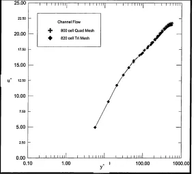
4.3.1 Fully developed channel flow... 60

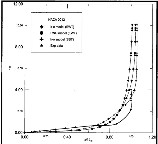
4.3.2 NACA0012 airfoil turbulent flow... 68

4.4 Summary... 72

Chapter 5’iua (Moat fjwuidfex. C51D Validation) 5tat tPEate Coaling. 74 Modeling. SMeaulto 5.1 Introduction... 75

5.2 Film cooling for a flat plate case (solid and shell) 75 5.2.1 Single film cooling hole... 75

• Geometry, mesh and boundary conditions 75 • Validation...of heat transfer CFD results... 76

5.2.2 Two rows of film cooling holes... 80

• Geometry,.mesh and boundary conditions... 80

• Validation of heat transfer CFD results... 82

5.2.3 Film cooling holes arrangement... 90

• Geometry, mesh and boundary conditions... 90

• Validation of heat transfer CFD results... 91

5.3 Summary... 101

Chapter Six SiladeQaa tJudtineC&S) Modeling <C Sleoulio 102 6.1 Introduction... 103

6.2 Essential independent turbine geometric parameters 103 6.3 Gas turbine blade and film cooling physical domain 107 6.4 Creating.the computational domain... 110

6.4.1 Blade meshing... 112

6.4.2 Mesh independent solution... 113

6.5 Boundary conditions... 115

6.6 Selecting solver, equation and solution convergence.... 117

6.7 Gas turbine results... 119

6.7.1 Effect of blowing ratio... 119

6.7.2 Effect of coolant temperature... 128

6.7.3 Effect of injection angle... 130

6.7.4 Effect of hole numbers... 132

6.8 Pressure coefficient and velocity vector for 3-D skewed

137 blade...

6.9 Summary... 140

Chapter Seven Sxp&umental Mvdduny, J'vepcwxtwn <£ Oledidts 143 7.1 Introduction... 144

7.2 Gas turbine blade geometry... 144

7.3 Gas turbine blade specimen manufacturing process 146

7.3.1 Laser sintering technology... 146

7.3.2 Process of direct metal laser sintering (DMLS) 147 7.3.3 Direct metal 20 description, application... 148

7.4 Experimental equipments... 149

7.4.1 K-type thermocouples... 150

• Thermocouple junction types... 151

• Grounded j unction... 151

• Ungrounded junction... 151

• Exposed junctions... 151

7.4.2 Pico USB TC-08 temperature data logger... 152

7.4.3 Thermal paint temperature technology (TPTT) 154 • Types of thermal paint... 155

• Thermal paint temperature calibration... 157

7.4.4 Air compressor... 158

7.4.5 Gas turbine unit... 158

7.4.6 Flow visualization and measurement system... 159

• Laser Doppler Anemometer (LDA)... 159

• Air flow meter... 160

7.5 Thermal wind tunnel design... 161

7.5.1 Speed region classification... 161

7.5.2 Tunnel geometry classification... 161

7.5.3 Thermal wind tunnel (TWT) CFD optimization 162

7.5.4 Uniformity of test section air velocity... 163

7.6 Preparation and Experimental test rig setup... 163

7.7 Experimental test procedure... 167

7.8 Accuracy of instrument and equipment... 170

7.9 Experimental Results Analysis... 171

7.9.1 Coolant fluid injected at 45° degree... 171

7.9.2 Coolant fluid injected at 60° degree... 178

7.9.3 Coolant fluid injected at 35° degree... 181

7.9.4 Thermal paint sensitivity for different angle of injection... 183

7.10 Experimental and numerical validation... 185

7.11 Summary... 186

CAaptek nine ConcCuaion and Steeanunendationa 188 8.1 Conclusions... 189

8.2 Future Work... 193

List of Figure

Figure (1-1) Components of gas turbine engine [Lu (2007)]... 2

Figure (1-2) Rolls Royce turbojet engine [Norman and Zimmerman (1948)]... 3

Figure (1-3) Rolls Royce AVON Turbojet Engine, [Rolls Royce online (2008)]... 4

Figure (1-4) Gas turbine thermodynamics [Brooks (2008)]... 5

Figure (1-5) Theoretical variation of specific fuel consumption and specific thrust for a real engine with compressor pressure ratio and TET [Sargison (2001)]... 6

Figure (1-6) Blade configurations for the convection cooling technique [Bathie (1995)]... 7

Figure (1-7) General impingement cooling technique [Boyce (2002)]... 8

Figure (1-8) Blade film-cooling [Bredberg (2002)]... 8

Figure (1-9) Transpiration cooling method [Bathie (1995)]... 9

Figure (2-1) Schematic of channel geometry... 17

Figure (2-2) Schematic representation of secondary flow and end-wall boundary layers [Kassim et ah (2007)]... 20

Figure (2-3) Schematic of the solid plane plate with the heater-foil, the coolant injection, cooling holes, the main gas flow, and some relevant physical quantities [Vogel and Graf (2003)]... 22

Figure (2-4) Research methodology and structure... 36

Figure (3-1) Cell center control volume for finite volume method A) structured mesh B) unstructured mesh... 41

Figure (3-2) Turbulent boundary layer universal velocity profile [Kravchenko et al. (1996)]... 47

Figure (3-3) FLUENT simulation structure [FLUENT (2006B]... 49

Figure (3-4) Two dimensional and three dimensional cell type [FLUENT (2006A)]... 50

Figure (3-5) Pressure based segregated algorithm [FLUENT(2006B)]... 53

Figure (3-6) Coupled solver method [FLUENT(2006B)]... 54

Figure (4-1) Fully developed turbulent channel flow for A) Triangular Mesh B) Quad Mesh [Daud etal. (2011 A)]... 59

Figure (4-2) NACA 0012 airfoil domain and Mesh [Daud et al (2011A)]... 60

Figure (4-3) Mean velocity profile: Mesh type effects for fully developed channel flow [Daud et al. (2011 A)]... 61

Figure (4-4) Mean velocity profile: Mesh type effects for fully developed channel flow [Daud et al. (2011 A)]... 61

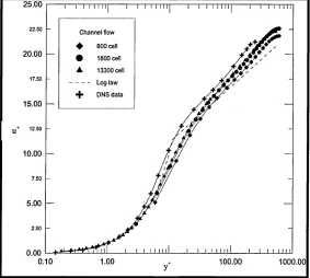
Figure (4-5) Mean velocity profile: Mesh refinement effects for different number of cells compared with DNS of Moser et al. (1999) at Rex = 590 [Daud et al. (2011 A)]... 63

Figure (4-6) Kinetic energy for different number of cells compared with DNS of Moser etal (1999) atRex= 590[Daud et al (2011A)]... 63

Figure (4-8) Mean velocity profiles: Mesh quality effects with and without boundary layer mesh (800, 820, 798, and 36 cells) [Daud et al

(2011 A)]... 65 Figure (4-9) Mean velocity profiles: Effects of Reynolds number (ReT= 590,

2320) [Daud et a l (2011 A)]... 67 Figure (4-10) Velocity gradients: Effects of Reynolds number (Rex= 590,

2320) [Daud et a l (2011 A)]... 68 Figure (4-11) Static pressure distribution for the Reynolds numbers Re=

4*105 compared with Sagrado (2007). [Daud et al (2011A)].. 69

Figure (4-12) Mean velocity profiles at X/Cx=0.55: different wall function effects (EWT and SWF). [Daud et a l (2011 A)]... 69 Figure (4-13) Mean velocity profiles at X/Cx=0.55 for k-s, RNG, and k- co

turbulent models. [Daud et al. (2011 A)]... 70 Figure (4-14) Kinetic energy (K+) at X/Cx=0.55 for k~s,_RNG and SSTk-oa

turbulent models. [Daud et a l (2011 A)]... 70 Figure (4-15) Numerical velocity at X/Cx=0.55 for k-e,„RNG and SST k-cd

turbulent models normalized with inlet velocity Uoc compared with Sagrado (2007). [Daud et al (2011A)]... 71 Figure (4-16) Numerical velocity at X/Cx=0.96 for k-e,,.RNG and SST k-co

turbulence models normalized with inlet velocity, Ua> compared with Sagrado (2007). [Daud et al (2011A)]... 72 Figure (5-1) Geometry and computational model [Liu et al 2008, Sinha et

al 1999]... 76 Figure (5-2) Static temperature contour of the single hole at BR = 0.5 (a) the

whole view, (b) zoom in [Daud et al (2012) impressed in Chanada]... 78 Figure (5-3) Local film cooling effectiveness for single hole at BR = 0.5;

comparison with the numerical/experimental results of Liu et

al (2008) and Sinha (1999)... 78

Figure (5-4) Geometry and arrangements of cooling holes along streamwise

direction Yuen and Martinz-Botas (2005)]... 80 Figure (5-5) Computational domain for mainstream, solid plate and coolant

holes and mesh generation... 81 Figure (5-6) Film cooling effectiveness trajectory along the plate through the

hole centerline at BR=0.5; A) Material thermal property effects;

B) Solid and shell plate effects [Daud et a l

(2012)]... 83 Figure (5-7) Static temperature contour through the holes centerline at BR =

0.5 [Daud et a l (2012)]... 84 Figure (5-8) The effectiveness cooling distribution contour at different

location for X/D=0, 1, 3 and 6 at BR = 0.5 [Daud et a l

(2012)]... 85 Figure (5-9) Effect of blowing ratio on the film cooling effectiveness

distribution (BR = 0.5 and 1) [Daud et al.

(2012)] 86

Figure (5-10) Streamwise velocity profiles at different location X/D=0, 1, 3

and 6 at BR= 0.5 and 1 [Daud et al.

(2012)]... 87 Figure (5-11) Mid of plate section velocity vector normalized by inlet

velocity at BR = 0.5 and 1 [Daud et a l

Material thermal property effects, B) Blowing ratio effects.

[Daud et al. (2012) impressed in Canada]... 89

Figure (5-13) Geometry and arrangements of cooling holes along the streamwise direction [Yuen and Martinz-Botas (2005)]... 90

Figure (5-14) The cooling effectiveness contour for the single row and double row of holes, P/D= 6 at BR = 0.5 with zooming section [Daud et al. (201 IB)]... 92

Figure (5-15) Spanwise distribution of local film cooling effectiveness at X/D=l, 3, 6 and 10 for the solid steel plate for single and double row at P/D= 6 with BR = 0.5[Daud et al. (201 IB)] 93 Figure (5-16) Local film cooling effectiveness along streamwise compared with experimental [Yuen and Martinz-Botas (2005)] for P/D=6 at BR = 0.5 and l[Daud et a l (201 IB)]... 94

Figure (5-17) The static temperature contour for coolant mainstream fluid, hot jet flow and steel plate at X/D=l for BR=0.5 and l[Daud et a l (201 IB)]... 95

Figure (5-18) Local film cooling effectiveness along streamwise compared with experimental Yuen and Martinz-Botas (2005) for P/D=3 at BR = 0.5 and 1 [Daud et a l (201 IB)]... 96

Figure (5-19) Film cooling effectiveness trajectory along the plate through the hole centerline for Solid and shell plate at BR=0.5. [Daud et a l (201 IB)]... 97

Figure (5-20) Film cooling effectiveness trajectory along the plate through the hole centerline; A) Material thermal property effects at BR=0.5; B) Effect of blowing increases from BR = 0.5 to 1. [Daud et a l (201 IB)]... 97

Figure (5-21) Local Nusselt number cooling distribution along the plate A) Material thermal property effects at BR=0.5; B) Effect of blowing increases from BR = 0.5 to 1. [Daud et al. (201 IB)]. 100 Figure (6-1) The five key points and five surfaces function [Pritchard (1985)]... 104

Figure (6-2) Leading edge and trailing edge tangency points [Pritchard (1985)]... 105

Figure (6-3) Types of gas turbine blade geometry generated off Pritchard’s program [Pritchard (1985)]... 107

Figure (6-4) Series of rotating turbine blades. [Coulthard (2005)]... 108

Figure (6-5) Actual blade model... 109

Figure (6-6) Computer Aided Measuring Machine (CMM)... 110

Figure (6-7) Assembly of gas turbine blade geometric model... 110

Figure (6-8) Blade geometric model... I ll Figure (6-9) Holes geometric model... I ll Figure (6-10) Flow diagram of exploring process starts from CMM to FLUENT data results... 112

Figure (6-11) Local mesh of blade model as a solid body with cooling holes system[Daud et al (2011C)]... 113

Figure (6-12) Multi block technique at meshing whole flow simulation box with blade model and holes film cooling... 113

Figure (6-13) Mesh refinement solution strategy for temperature, pressure and velocity along the blade surface as gradient variables... 115

Figure (6-15) Predicted counters temperatures of the blade model at different blowing ratio A) BR=1, B) BR=1.5, C) BR=2 [Daud et al.

(2011C)]... 120 Figure (6-16) Temperature and the Effectiveness cooling distributions

difference in hub, mid and shroud area on the blade model by injecting coolant air at BR=2 [Daud et al. (2011C)]... 122 Figure (6-17) Effects of blowing ratio (BR) on the blade effectiveness

cooling- A) hub, B) mid and C) shroud [Daud et al. (2011C)]... 124 Figure (6-18) Film cooling effectiveness couture at blowing ratio BR= 2 on

the blade model [Daud et al. (2011C)]... 125 Figure (6-19) Distributions of film cooling effectiveness at blowing ratio

BR=1 at angle of injection 35°: comparison between CFD results of Burdet et al (2007), the blade model calculation [Daudetal. (2011C)]... 125 Figure (6-20) Predicted profile of Nusselt number (Nu) at midspan for BR=1,

1.5, 2 [Daud et a l (2011C)]... 126 Figure (6-21) Nusselt number (Nu) counter on the blade model for BR=2

[Daud et al. (2011C)]... 127 Figure (6-22) Effects of coolant fluid temperature on the film cooling

effectiveness at BR=1, 1.5... 129 Figure (6-23) Effects of coolant fluid temperature on the temperature

distribution BR=1.5 at 35 angle of injection... 130 Figure (6-24) Effects angle of injection at mid area with different (BR) on

the blade effectiveness cooling... 131 Figure (6-25) Effects of injection angle on gas turbine temperature

distribution at blowing ratio BR= 1... 132 Figure (6-26) Cooling effectiveness trajectory at B R=1.5 for hub, mid and

shroud area effected by number of holes... 134 Figure (6-27) Effects of holes number on gas turbine temperature distribution

at blowing ratio BR=1.5 with angle of injection 45°... 135 Figure (6-28) Cooling effectiveness trajectory at B R=2 for hub, mid and

shroud area effected by holes diameter... 136 Figure (6-29) Effects of holes diameter on gas turbine temperature

distribution at blowing ratio BR=2 with angle of injection 45°... 137 Figure (6-30) Pressure coefficient distribution for gas turbine blade with 45°

angle of injection at BR°=2... 138 Figure (6-31) Velocity vector for gas turbine blade with 45° angle of injection

at BR°=2 for A) Hub B) Mid C) Shroud... 139

Figure (7-1) Gas turbine blade specimen model dimension and cooling holes

position with projection side views... 145 Figure (7-2) EOSINT M 280 direct metal laser sintering machine [BMT,

online]... 146 Figure (7-3) A schematic diagram of the EOS machine [Custompartnet,

online]... 147 Figure (7-4) Gas turbine specimen fabricated in EOSINT M 250 X tended

systems... 149

Figure (7-5) K-type thermocouples operation principle [Pico, online] 150

Figure (7-6) Thermocouple probe junction types, (A) grounded, (B)

ungrounded and (C) exposed [Eutechinst,

Figure (7-7) K-type stainless steel thermocouple probe at 0.5 mm diameter with miniature plug... 152 Figure (7-8) Pico TC-08 data logger device... 153 Figure (7-9) Calibration process for cooper pipe with furnace and KN 5

coupon calibration... 157 Figure (7-10) Air compressor device... 158 Figure (7-11) Panel board for gas turbine unit ... 159 Figure (7-12) Laser Doppler Anemometer (LDA) system principle [Dantec,

online]... 160 Figure (7-13) Rotameter airflow meter type... 160 Figure (7-14) Thermal wind turbine (TWT) designed in pro/Engineer

Wildfire (CAE) package... 162

Figure (7-15) Pressure and velocity contour for additional parts of TWT 162

Figure (7-16) Full Thermal wind Tunnel (TWT) manufactured design... 163 Figure (7-17) Preparation process steps to finalize TWT... 164

Figure (7-18) Thermocouples (K type) concealed in gas turbine blade 165

Figure (7-19) Illustrates gas turbine blade coated by thermal paint (KN5) and thermal paint on vibrator machine... 166 Figure (7-20) Setup process of thermal wind tunnel, fixed gas turbine

specimen in test section, inserting thermocouples, coolant air supplier and calibrates levels to be horizontal... 167 Figure (7-21) Schematic of film cooling test rig and data acquisition system... 167 Figure (7-22) Experimental measurements of mainstream velocity at the inlet

of test section utilizing by LDA... 169 Figure (7-23) Process of scaling thermal paint from blade specimen using

Chloroform solvent and 30% of Nitric acid... 169 Figure (7-24) Percentage error bar for inlet and outlet test section temperature

measurements point at thermocouple (1) against time... 171 Figure (7-25) Inlet and outlet test section temperature with five core blade

temperature against time... 172 Figure (7-26) Effects of V° on film cooling effectiveness at A) measurement

point (1) and B) measurement point (2)... 174 Figure (7-27) Average of film cooling effectiveness for the last 30th point of

measured temperature for each location at holes angle of injection 45° for A) V°=1000, V°=800 and V°=600 (cm3/min)... 176 Figure (7-28) Blade surface temperature distribution patterns coloured by

thermal paint with V°= 1000, 800, 600 (cm3/min)... 178 Figure (7-29) A) Transient temperature thermocouple measurements at

V°=1000 cm3/min, B) Temperature difference between pressure side and suction side... 179 Figure (7-30) A) Effect of varying BR on film cooling effectiveness against

time for holes angle of injection 60° B) Average film cooling effectiveness measurements along the blade at the mid region V°=1000 cm3/min... 181 Figure (7-31) A) Transient temperature thermocouple measurements at

V°=1000 cm3/min, B) Temperature difference between pressure side and suction side... 182 Figure (7-32) Average film cooling effectiveness measurements along the

Figure (7-33)

Figure (7-34)

Blade surface temperature distribution patterns coloured by thermal paint for holes injection at 45°, 35° and 60° at V°=

1000(cm /min)... 184

List of Table

Table 3-1 GAMBIT face meshing element options [FLUENT(2006A)]... 50

Table 3-2 GAMBIT face meshing type options [FLUENT(2006A)]... 50

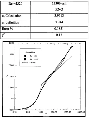
Table 4-1 The values of numerical and defined shear velocity at Rex=590... 67

Table 4-2 The values of numerical and defined shear velocity at Rex=2320... 67

Table 5-1 Comparison of CFD data, experimental data and previous

numerical data at X/D=3... 79 Table 5-2 Comparison of CFD data, experimental data Sinha (1999) and

previous numerical data Liu et al (2008) at X/D=6... 79 Table 5-3 Solid plate material properties... 81 Table 5-4 Solid plate material properties... 91 Table 5-5 Nnumber of cells for each numerical simulation (single hole, two

row of hole and holes arrangement) at solid and shell case with consuming time... 101 Table 6-1 Application of boundary conditions... 116

Table 6-2 Inlet hot gas and cooled air applied to FLUENT software 117

Table 6-3 The average film cooling effectiveness values at the mid area on

pressure side gas turbine blade... 141 Table 6-4 Computational time with number of cells for 3 D skewed gas

turbine blade simulations at different angle of injection 35°, 45° and 60° respectively... 142 Table 7-1 Material property of direct metal 20[EOS (2004)]... 148

Table 7-2 Common thermocouple temperature ranges [Omega,online] 151

Table 7-3 Lists the specification of the TC-08 data logger [Pico online] 153

Table 7-4 Single change paints sorts [TPTT]... 156 Table 7-5 Multi-change paints sorts [TPTT]... 156 Table 7-6 Temperature and colour density for each color transition. [TPTT]. 157 Table 7-7 Experimental test boundary conditions... 170 Table 7-8 Percentage error of measurement equipment... 170 Table 7-9 Average temperature values and difference... 173 Table 7-10 Film cooling effectiveness values for each V° at the last 30th

point... 176

Table 7-11 Average thermocouple temperature for all V°. and both sides 180

Table 7-12 Average thermocouple temperature difference for all V°. and both

Nomenclature

A Projected area of the cell

BR Blowing ratio, BR = pc *VC / px * Vx

CP Static pressure coefficient distribution, equation (4-7)

Cp, (Cp)s Specific heat the for the fluid flow, solid body

Cx the blade axial chord (mm)

Cy the blade width (mm)

Cz the blade spanwise (mm)

D Film hole diameter (mm)

Dh Hydraulic diameter (mm) in equation (6-2)

Gb general turbulence kinetic energy due to buoyancy

Gk general turbulence kinetic energy due to the mean velocity gradients

H channel width (m)

9 9

k turbulence kinetic energy (m Is )

K, K s thermal conductivity for fluid flow, solid body (W/m-K)

K+ dimensionless turbulent kinetic energy based on uT ,equation (4-2)

K-Locai local kinetic energy, KL0Cai= ■ +. /d y +

j J T C f c i

L length of the film hole or length of channel flow (mm)

L mixing length is presumed known in turbulent viscosity

/ length scale (m)

I£ mixing length for EWT based on turbulent rate of dissipation (m)

/ mixing length for EWT based on laminar viscosity (m)

rn Mass flow rate (kg/sec)

Nu Nusselt number

P Pressure (N/m )

Poi inlet total pressure. (N/m2)

Ps static pressure on the surface (N/m2)

Ps2 outlet static pressure (N/m2)

Pr> Prt laminar and turbulent Prandtl number

q* heat flux (W/m2)

Re free stream Reynolds number

(Rex) friction Reynolds numbers based on uT, Rex= (p*ux*H)/p

R.j Boussinesq relationship equation (3-10)

Sy stress tensor.(l/sec)

T temperature (K)

AT temperature difference

Tc injection film cooling temperature (K)

Too mainstream temperature(K)

Tu turbulent intensity, equation (6-1)

ut averaged velocity components (m/sec)

+

u dimensionless mean velocity based in the wall unit, u+ =u/uT

ur friction velocity, uT = Jtw / p (m/sec)

K mainstream velocity (m/sec)

Vc coolant velocity (m/sec)

X,Y,Z Spatial coordinates (mm)

+

y dimensionless distance from the wall to nearest grid cell(y+=p uTy/p) Pc ’ Poo Coolant fluid and mainstream density, (kg/m3)

d ( X T~r\ Reynolds stress (closure).

dP/dx Pressure gradient

d / dxj represents the variation of parameters in X, Y and Z

s Turbulent rate of dissipation

P,Pt dynamic viscosity,turbulence (or eddy) viscosity (kg/m.sec) s , Kronecker delta function (equal to one if i = j , else zero)

wall shear stress (kg/m. sec )

e velocity scale (m/sec)

Abbreviations

AoA Angle of Attack

B.C B oundary Condition

B.L Boundary Layer

CFD Computational Fluid Dynamics

CHT Conjugate Heat Transfer

CMM Computer Aided Measuring Machine

DES Detached Eddy Simulation

DNS Direct Numerical Simulation

EWT Enhancement Wall Treatment

FVM Finite-Volume Method

IGES Initial Graphics Exchange Specification

IR Infrared Thermography Method

LCT Liquid Crystal Technique

LDA Laser Doppler Anemometer

LDV Laser Doppler Velocimetry

LES Large-eddy Simulation

MRF Micro-Riblet Film

MTU G erm any’s leading aircraft engine manufacturer

MUSCL Monotone Upwind Scheme for Conservation Laws

PDE Partial Differential Equations

PIV Particle Image Velocimetry

PS Pressure side

PSP Pressure Sensitive Paint

RANS Reynolds Averaged Navier-Stokes

RNG Re-Normalization Group RNG Model

RP Rapid prototyping

RSM Reynolds Stress turbulence Model

S-A Spalart- Allmars Turbulence Models

SFC Specific Fuel Consumption

SIMPLE Semi-Implicit Method for Pressure Linked Equation

SS Suction side

SST Shear Stress Transport

ST Specific Thrust

SWF Standard Wall Function

TET Turbine Entry Temperature

TLV Two Layer Velocity Scale Model

TLVA Anisotropic Two Layer turbulence model and DNS Based Model

TLVA-Pr Anisotropic two layer turbulence model and DNS based Model of Pr in the boundary layer

TPTT Thermal Paint Temperature Technology

TWT Thermal Wind Tunnel

1.1 General introduction

A Gas Turbine (GT) is a device used for converting thermal energy into mechanical energy in the form of reaction of the runner, under high pressure and then discharging the gas in the desired direction [Norman and Zimmerman (1948)].

As shown in Figure (1-1), a typical gas turbine engine comprises of three main components, namely the compressor, combustor and turbine [Nasir (2008)].

turbine

exhaust

air intake combustion

chamber

Figure (1-1) Components of gas turbine engine [Lu (2007)]

Gas turbines has been developed for a number of applications; including, electrical power generation, aircraft propulsion, industrial gas turbine engines, naval vessels propulsion and trains.

increased number of explosion chamber [Oberg and Jones (1917)]. The objective has been to enhance the overall efficiency, reduce the consumption of fuel and increase thrust in the aircraft engine. So, a brief historical review will be made of gas turbine innovations and designs

1.2 International historical perspective of patents

1.2.1 British efforts

In England, gas turbines were constructed and tested to power airplanes by two research groups. The first group, led by Frank Whittle, concentrated on the turbojet using the centrifugal flow compressor. The second group, led by Griffith at Liverpool, worked on testing and constructing the axial flow compressor. Whittle's group achieved the first patent in 1930; however this project was not accepted by the Air Force Ministry and private companies since it was deemed to be a long term research project and adequate funding was not available. However, in summer 1939 the Air Force Ministry signed a contract for the power jet. In 1936, the Griffith group in England began work with the Royal Aircraft Establishment on constructing and testing axial flow compressors. Through a series of research efforts, the UK completed the first airplane flight powered by the gas turbine in 1941, [Bathie (1995)]. Figure (2-1) illustrates the first turbo jet engine.

Since that time, competition between many companies has continued. For example Rolls-Royce and Pratt and Whitney (USA) produced several gas turbines to increase performance. Figure (1-3) shows the Avon turbojet engine, developed by Rolls- Royce.

Figure (1-3) Rolls Royce AVON turbojet engine, [Rolls Royce, (2008)]

1.2.2 French efforts

Bresson idea was to drive pressurized air in a combustion chamber by using a fan. The air was mixed with the fuel gas and then combusted. Additional air was used to cool the combustion products before delivery to the turbine blades [Giampaolo (2006)].

1.2.3 German efforts

1.2.4 USA efforts

Historically, the National Advisory Committee for Aeronautics (NACA) used the work of S. Campini from 1930 onwards. They designed a ducted axial fan motorized by the reciprocating engine. The efficiency of turbines and the compressor was not well developed at this time. However, in 1939 Brown Boveri built the first commercial gas turbine power plant for generating power (4000 kW). In the United States in 1940, the 2500- hp turboprop engine was developed for the US Army and US Navy. Since this time, the USA has led developments in the design and building of many gas turbines, many of which are reported in the ASME Journal of Gas Turbines and Power Journal [Bathie (1995)].

However, these efforts are aims to increase the thrust, overall efficiency and reduce the fuel consumption, as much as possible, by increasing the turbine inlet temperature. (Combustor exit temperature) as illustrated in Figure (1-4).

SIMPLE CYCLE

EXHAUST

ELECTRIC

POWER

[ O y J

COMBUSTOR /

12 PRESSURE RATIO Xj

250T‘-0227)(12M) , T,»FPC)

GENERATOR TURBINE

COMPRESSOR

0.140 0.150 0.160 0.170 0.180

(.064) (.066) (.073) (.077) (.082)

SPECIFIC OUTPUTMW/lb/*ee (M W /kfl/S)

COMBINED CYCLE EXHAUST PRESSURE RATIO Xc .53 GENERATOR

'H O C

HRSG

AR _STEAM

TURBINE

- d *_GENERATOR

0.16

(0-35) (0.44)0.20 COMPRESSOR

HIGHER TEMPERATURE MEANS MORE POWER

SPECIFIC OUTPUT MW/ lb/m c (M W /kg/S) HIGHER TEMPERATURE SAVES FUEL

Figure (1-4) Gas turbine thermodynamics [Brooks (2008)].

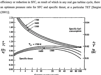
Specific Fuel Consumption (SFC) and furthermore Specific Thrust (ST) with Turbine Entry Temperature (TET) and compressor pressure ratio. The increase in the TET at a constant pressure ratio through a change in fuel/air ratio causes an increase in the specific work output, or specific thrust. However, this variation does not change the overall efficiency of the engine. Additionally, increasing the compressor pressure ratio (which has the effect of increasing TET at constant fuel/air ratio), causes an increase in efficiency or reduction in SFC, as result of which in any real gas turbine cycle, there is an optimum pressure ratio for SFC and specific thrust, at a particular TET [Sargison

(2001)].

2.20 1700 1600 1500 2.00 0.04 1.40 1.20 F

T . = 1700 K

1.00 0.02 1500 0.80 ₁₆₀₀ 0.60 0.01 Specific thrust 0.40 0.20 0.00

30 40 60 80 a00 Compressor pressure ratio

F kB kN-s

Figure (1-5) Theoretical variation of specific fuel consumption and specific thrust for a real engine with compressor pressure ratio and TET [Sargison (2001)]

Unfortunately, higher temperatures have negative effects on the integrity of high pressure turbine components and materials comprising the turbine blades [Kassim et al.

(2007)]. Designers of gas turbines have resolved the problem of blade surface degradation and rapid failure from high inlet temperatures by using blade cooling technology. In this dissertation, numerical and experimental methods are used to examine the flow in a high-pressure gas turbine chamber in order to investigate blade film cooling.

1.3 Gas turbine cooling method

In this method, the coolant (air) flows outward from the base of the turbine blade to the end through internal passages within the blade [Bathie (1995)]. Figure (1-6) illustrates several passageways for the convection cooling technique. The quantity of cooling air and the size of internal passages are the greatest limitation on the cooling effectiveness of the convection method. Therefore, high velocity and internal surface areas are essential for the coolant air. An additional major disadvantage of convection cooling is that no cooling air passes through the thin trailing edge of the blade [EL-Sayed (2008)].

tooting

Figure (1-6) Blade configurations for the convection cooling technique [Bathie (1995)].

1.3.2 Impingement Cooling Method

Figure (1-7) General impingement cooling technique [Boyce (2002)].

1.3.3 Film Cooling Method

As illustrated in Figure (1-8), the film cooling method is as an external cooling technique. It involves injection of a secondary fluid from the inside of the blade into the boundary layer of the primary hot gas through a number of holes [Peng (2007)].

Internal air system

PIN-FIN SYSTEM IM PING EM ENT TUBES

TURBULATOR RIBS

PLATFORM FILM COOLING HOLES

Cooling air

Figure (1-8) Blade film-cooling [Bredberg (2002)].

penetrate the incoming flow, counter-acting the purpose of film cooling, as turbine losses will occur. However, film cooling is a more effective method than standard convection, or impingement cooling, since it does provide a protective layer along the surface of the blade.

1.3.4 Transpiration Cooling Method

As shown in Figure (1-9), the coolant air is blown (injected) through a porous blade surface to achieve full blade film cooling. The transpiration cooling method is effective at very high turbine inlet temperature as the pores cover the entire blade with coolant air [Boyce (2002)].

Hot stream

Cooled air

Figure (1-9) Transpiration cooling method [Bathie (1995)].

1.4 Technology of cooling blades in a gas turbine

The phenomenon of jet-in crossflow (coolant fluid) which is a characteristics of film cooling, results in mixing in shear layer which reduces the surface temperature of the blade i.e. enhance the film cooling effectiveness [Bogard and Thole (2006)]. Hence, characterization of the gas flow and heat transfer through a modem turbine are important engineering considerations, as they which represent very complex flow fields and high turbulence levels. In the first stage of turbine blade design, it is crucial to reduce the over-heating effect on the blade surface. A disadvantage of this technique is a source of loss in the overall power output since coolant fluid has to be extracted from the compressor. Approximately 20-25% of compressed air bleeds to the cooling system [Ekkad et al. (2006)]. Despite this, the benefits in reduced SFC and increased specific power output which follow from an increase in permissible TET (combined with an increase in compressor pressure ratio) are still substantial when the additional losses introduced by the cooling system are taken into account [Sargison (2001)]. Therefore, optimum cooling technology can be influenced by the following parameters:

A). Selection of a method to protect gas turbine elements from thermal overheating by using an air efficient cooling system which may be either internal cooling (convection cooling system or impingement cooling system) or external cooling (film cooling system or transpiration cooling system)[EL-Sayed (2008)].

B). Selection of a suitable coolant fluid (water or air).

C). The degree of cooling air (characterized by mass flux ratio which is simulated by a Blowing Ratio (BR).

BR = pc *VC!pm *VX

Where

■j

pc is a coolant fluid density, (kg/m )

Vc is a coolant velocity (m/sec)

px is a mainstream density, (kg/m )

V{M is a mainstream velocity (m/sec)

D). The injection angle (lateral injection, stream-wise inclined and span-wise).

E). The discharge geometry (number of holes, diameter of the holes and row of holes).

research will be concerned with performance of gas turbine through study aerodynamic and heat transfer numerically and experimentally. Different parameters i.e. effects blowing ratio, cooling temperature, angle of injection, number of holes and holes diameter are mainly interest with the optimum performance of gas turbine blade.

1.5 Aim of the research

This research is mainly concerned with the performance of gas turbines. Numerical and experimental methods are used to examine the flow in a gas turbine chamber in order to investigate blade film cooling. Aerodynamic flow and heat transfer rates are computed using numerical and experimental methods. The optimization process examines film cooling blade design (blowing ratio, angle of injection). Moreover, channel flow, NACA 0012 airfoil and flat plate were used to investigate the performance of FLUENT code solver through explain the restrictions in fundamental turbulent flow simulations and mesh generation. The research will calculate pressure drop, Nusselt number and cooling effectiveness at three key locations and show effect of cross section area variation in gas turbine blade on film cooling performance, namely the hub, mid and shroud.

1.6 Objectives of the research

experimentally with a Thermal Wind Tunnel (TWT). Therefore, the main objectives of the present thesis are:

1. Validation of numerical calculations inside channel flow and above a NACA 0012 airfoil using FLUENT code with available numerical and experimental published data.

2. Verification of the amount of heat transfer and film cooling for a flat plate surface simulated as a solid and shell. The simultaneous calculation of conduction and convection is called Conjugate Heat Transfer (CHT). The conjugate approach involves time-consuming computation as the number of grid points increase as both fluid and solid domain have to be taken into consideration [Kane and Yavuzkurt (2009)]

3. Identification of useful parameters to satisfy high film cooling effectiveness on gas turbine blades with FLUENT simulation. This involves:

A) Generation of a Cartesian-coordinate based geometric model of a gas turbine blade geometry at the three main areas (hub, mid and shroud), using the pre­ processor (generating the meshing using GAMBIT tool). A size function tool will be used to control the model meshes by creating a regular size of mesh intervals for edges, elements, faces and volumes [FLUENT (2006A)].

B) Application of the FLUENT Computational Fluid Dynamics (CFD) software to simulate fluid flow and heat transfer in the turbine geometry.

4. Validation of numerical results using published data and previous related work 5. Conducting experiments on fabricated blade test sections and analyzing

experimental results to validate numerical results.

1.7 Motivation of the research

curved boundary, namely the NACA 0012 airfoil, in order to explore aspects relevant to gas turbine geometries which can then be validated with experimental data. Having established confidence in the computational code, we next examine the first case of gas turbine simulation, namely flat plate film cooling with different hole arrangements and consider blowing ratio and other effects, validating the new computations with experimental results from the literature. The next stage is then to simulate the film cooling performance in a realistic 3-D skewed gas turbine blade model, and to conduct experiments for this configuration. Consequently, the motivations of this research are:

Firstly, to assess restrictions of the FLUENT code solver in fundamental (and therefore more advanced) turbulent flow simulations. The aim is to investigate the relative accuracy of three different turbulence models (k-s,..RNG, SST k-co) in the numerical analysis. Furthermore, this thesis will explore the strong influence of mesh refinement and mesh type near the wall and outer layer turbulence structures on the flow characteristics for the two test cases of turbulent channel flow and turbulent NACA 0012 airfoil flow.

Secondly, numerical predictions of film cooling effectiveness, heat transfer, temperature distribution for a flat transpiring plate, will be investigated, by focusing on:

• The mainstream (hot gas) and coolant system (cooled fluid) with differences in temperature, pressure and chemical composition for the hot gas and cooled air. • Solid plate thermal properties which will be simulated by choosing the type of

manufacturing blade material for example, steel, carbon steel (SAE4140), aluminum, copper, and carbon steel shell plate into the FLUENT software property specification pre-processor.

Finally, this study is utilizing a complex geometry for a 3-D skewed solid blade to numerically investigate film cooling effectiveness, heat transfer, temperature distribution and the effect of coolant fluid property in the hub, mid and shroud area. In addition, experimental wind tunnel blade cooling tests are conducted. Therefore, this study will present the following aspects:

• Addressing solid body thermal properties which will be simulated by utilizing the type of blade material for example, carbon steel (SAE4140) in the FLUENT software property specification pre-processor.

2.1 Introduction

As mentioned in chapter one, the historical efforts in design and development have been aimed to increase thrust and thermal efficiency by increasing inlet temperature of gas turbines and employing efficient methods (e.g. cooling method) to protect gas turbine component by reducing blade surface degradation.

In order to accomplish the numerical and experimental study of flow in a gas turbine successfully this chapter will review gas turbine innovations, designs and recent research through a series of investigations. A discussion of the computations performed with the FLUENT code for wall-bounded turbulent flows in a two-dimensional channel

and boundary layer flow along a NACA airfoil are presented which are popular

benchmarks in computational fluid dynamics (CFD). Simulations of the amount of heat transfer along a flat plate using film cooling holes is a simplified model of relevance to the more geometrically complex case of jet-crossflow in 3-D skewed gas turbine blade model. Most of previous studies have concentrated on numerical and experimental analysis, namely, film cooling holes configurations and heat transfer from flat and curved plates. Fundamentally, heat transfer to turbine blades involves steady heat transfer based on mean-flow conditions, as well as unsteady heat transfer due to fluctuations in the mean flow [Nix (2003)]. For film cooling in gas turbine blades there is the additional complexity of flow around the blade (jet-cross-flow). Again, the objective of the cooling design is focused on computing the heat load to extend component life, to minimize coolant air and optimize the performance of gas turbine blades.

2.2 Fluid flow analysis

turbulence models (for example, k-epsilon, K-omega), thereby demonstrating the best models for implementation in terms of accuracy and compilation times.

2.2.1 Wall bounded turbulence

Channel flow was selected as one of the two fundamental flow regions studied to aid in numerical simulations discussed in later chapters. This flow region is common in many branches of mechanical engineering including power generation, propulsion, materials processing, rocket chamber flows. The characteristics of flow inside channels are strongly related to the wall effects and the Reynolds number. A number of excellent studies examined such flows both numerically and experimentally. Figure (2-1) illustrates a schematic of the channel geometry studied.

Figure (2-1) Schematic of channel geometry.

Iwamoto et al.{2005) presented a fully-developed turbulence channel flow study utilizing Direct Numerical Simulation (DNS) at Rex = 2320, using 16 billions node points and showing that mean velocity profile results compared with earlier studies for ReT = 650 and 150, respectively. However, this study indicated that at 100< y+< 600, the velocity profile in this region does not follow the logarithmic law, in addition to near wall turbulence depends on both fme-scale structure and large-scale structure (y+ is a non-dimensional distance similar to local Reynolds number, often used in CFD to describe the coarseness or fineness of a mesh for a particular flow). It is the ratio between the turbulent and laminar influences in a cell [Salim and Cheah (2009)]. This study showed that the trajectory of KLocai (local kinetic energy) gradually declines with increasing friction Reynolds number (ReT).

KLoca1"" (2-1)

Moser et al. (1999) conducted a DNS turbulent channel flow study, with Rex (friction

Reynolds number varied from 180, 390 to 590). The results suggested that the ReT= 590 flow simulation was at sufficiently large Reynolds number to be free of the most obvious low-Reynolds number effects. The authors obtained excellent correlation of results for the mean velocity profile up toy+~ 200 with the logarithmic law, for friction Reynolds number values of 590 and 390; however they identified deviation for Rex =

180 due to low Reynolds number effect.

Kim et al. (1987) performed a fully spectral DNS study for 3D incompressible turbulent

channel flow at low Reynolds number (Re) at the channel center at 3300 and the friction Reynolds number Rex=180, with grid 192*129*160 in the x, y, z directions. The first grid point away from the wall is y + = 0.05. Turbulence statistics were computed and compared with the experimental data. Special attention was given to the turbulence behavior near-wall.

Daud et al. (2011 A) investigated numerically the effects on turbulence for two important flow regions -fully developed channel flow and flow past a NACA 0012 airfoil, using commercial software - FLUENT 6.3. The solution accuracy was explored via a sensitivity study of mesh type and quality effects, employing different element types for example, quadrilateral and triangular. This work elucidated the effects of Enhancement Wall Treatment (EWT) and Standard Wall Function (SWF) on the turbulent boundary layer. Furthermore, four different turbulence models were utilized in this study, namely, S-A, k-g, RNG and SSTk-co. The numerical solutions were compared with available DNS results by Moser et al. (1999) and experimental data by Sagrado (2007). Good correlation was achieved. In addition, the statistical turbulence results related to the RNG turbulence model were shown to yield much closer correlation with DNS and experimental data. The effect of Reynolds number (Rex = 590 and Rex = 2320) were studied for the channel flow region and the near wall resolution examined in detail by controlling in the y+ value.

measurements were performed for the Reynolds number ranged from 1.03*104 to 5.14*104. However, the drag force on the MRF, which covered the airfoil, was about 6.6% lower than that on the smooth airfoil at Reynolds number Re=1.54*104. At high Reynolds number Re = 4.62* 104 ’ the drag force increased by 9.8% for MRF. The Particle Image Velocimetry (PIV) technique and ensemble averaged was utilized to measure the distributions of turbulence intensity and turbulent kinetic energy including the mean velocity through 500 instant velocity fields behind the airfoil, in addition to a smoke wire flow visualization technique. The results for the case of drag reduction

(Re=1.54*104) had a shorter vortex formation region and higher vertical velocity component, compared with smooth airfoil. Conversely, for the increased drag case (Re = 4.62* 104), the presence of MRF grooves on the airfoil were observed to increase the vertical velocity component and decrease the height of the large-scale streamwise vortices which interacted strongly. Thus, indicating an increase in the Reynolds shear stress and turbulent kinetic energy leading to higher drag force on airfoil.

Sagrado (2007) performed experiments in which pressure fluctuations and velocity field were measured in the tripped and untripped turbulent boundary layer on a NACA 0012 airfoil surface. In this study, attention was focused on the trailing edge zone. Different Reynolds numbers (Re) and angles of attack (a) were examined, specifically Re= (4, 2)*105 and a= 0°, 12.6°, 16° degrees respectively. In addition, the study included low and moderate Reynolds number studies for untripped boundary layers and high Reynolds numbers for the tripped boundary layer case, which can also play an important role in validation of Large Eddy Simulation (LES) and DNS models.

2.2.2 Aerodynamics of gas turbines

This section briefly reviews previous aerodynamic flow studies of the gas turbine blades. Actually, the flows in turbomachines have both steady and unsteady

(2-2) shows illustrates the secondary flow and end-wall boundary layers in gas turbine flows.

Endwall Inlet Boundary Layer

Tliick and Turbulent

Midspan

Three-Dimensional Separation Lines

Passage Vortex New Boundary Layer

Tliin and Higlily Skewed

Figure (2-2) Schematic representation of secondary flow and end-wall boundary layers [Kassim et al. (2007)]

Djouimaa et al. (2007) studied two-dimensional flow for the blade-to-blade transonic gas turbine, using an irregular structured grid and the FLUENT 6.0 software with a Reynolds Averaged Navier-Stokes (RANS) model. The characteristics of the flow were compared with experimental tests and included reflecting and non-reflecting boundary conditions. Different turbulence models (k-s, RNG k-8, Realizable k-s, SST k-co) were also examined to compute the pressure distribution around the blades, with the inlet Reynolds numbers (0.5-1.0)*106 and exit Mach numbers (1.0-1.3). The RNG model was employed in particular to show the effects of inlet turbulence intensities, exit Mach number and inlet Reynolds numbers.

moderately with increasing Reynolds number. The exit measurements also elucidated further the end-wall heat transfer distributions, the secondary flows in the passage and the losses.

Mei and Guha (2005) developed numerical simulations for turbine cascade and compressible transonic flow, using a self-adaptive, unstructured mesh. The Euler and Navier-Stokes equations were applied in the numerical program. Turbulence was simulated with an algebraic Baldwin-Lomax turbulence model, and the two-equation turbulent model (k-o) model) with high order accuracy through applied MUSCL approach. The Gauss-Seidel algorithm was used to solve the linear equations for each time iteration. Good correlation was obtained between the numerical and experimental results.

Michelassi et al. (1998) investigated boundary layer and wake flow in a transonic turbine rotor cascade, numerically and experimentally. Measurements included pressure and total pressure profiles for the blade in addition to isentropic Mach number. Computations were performed by FAST 3DC and FLOW3D solvers with different turbulence models (k-co and two layer model TLK) and three different transition models. The results provided a realistic description of the flow field allowing the calculation of pressure distribution and shock boundary layer interaction induced by small flow separation on the suction side which is generated due to transitions models. The experiments also indicated the presence of trailing edge vortices.

Chmotine et al. (1997) used the 2-dimensional Euler equations to model high pressure turbine flow in an aircraft engine. This study was based on the large-particle method, which is a numerical method for the stator and rotor blade; the unsteady effect was represented for the rotor blades moving along the fixed grid and the pressure and absolute total temperature were calculated on the rotor blade surface.

actual gas turbine geometries, and the Fluent computations are compared with available experimental data from Cambridge University.

2.3 Heat transfer and film cooling studies

2.3.1 Flat and curved plates

Figure (2-3) shows cooling region for a solid plane plate with the heater-foil, the coolant injection, cooling holes, the main gas flow, and relevant physical quantities. Many important studies of “film cooling” have been conducted.

M a i n f l o w

T tc(t)

t o = 0 t im e to = 0 t im e

Figure (2-3); Schematic of the solid plane plate with the heater-foil, the coolant injection, cooling holes, the main gas flow, and some relevant physical quantities [Vogel and Graf (2003)]

results by Yuen and Martinez-Botas (2005) and good correlation has been achieved. The effects of material thermal properties for the solid plate have been elucidated, in addition to variation concepts between the shell plate and the solid plate, on the film cooling effectiveness.

Nemdili et al. (2011) investigated the influence of film cooling holes imperfection on flat plate numerically with a symmetrical single perpendicular hole exhibiting jet flow. Numerical calculations were performed with the Reynolds Average Navier Stokes and an energy equation using the finite volume method to predict hydrodynamic flow and thermal effects. In addition, turbulence closure was achieved via the standard wall function k - s model. The simulation process was executed with the CFX 10 software package and the computational domain modeled as a structured mesh. Four imperfection hole cases were studied with 0%, 23.44%, 43.75% and 60.94% obstruction. Good agreement was obtained between numerical computations and the experimental results of Jovanovic et al. (2006). However, cooling effectiveness value was found to decrease quickly when the obstruction is higher than 50% and occurred close to holes exit implying that thermal protection for the blade was profoundly reduced.

Ghorab (2010) presented schemes of louver and hybrid film cooling performance over a flat plate experimentally using the Thermochromic Liquid Crystal Technique (TLC). The louver scheme (proposed in Canada) involves the film hole design allowing coolant fluid to pass through a bend and to encroach plate material (impingement effects) and then exit to the outer surface. This study aimed to evaluate the film cooling effectiveness and heat transfer at blowing ratios of 0.5, 1 and 1.5. In addition, a hybrid scheme was deployed to analyze the flow pattern at different blowing ratios. It was shown that the hybrid film hole allows the coolant fluid to be directed to the secondary flow in the horizontal direction and reduces the jet liftoff at different blowing ratios. Both louver and hybrid scheme provides high local film cooling and reduction in net heat flux compared with previous work. Moreover, enhancement in the film cooling of holes is obtained further along the spanwise direction.

techniques were also employed to obtain the measurements for two blowing ratios (1,2) with four swirling motions of the coolant. The results showed that the cooling effectiveness is strongly enhanced due to swirling effects due to the interaction between coolant film jets, mainstream and swirling motion (coolant fluid is deflected in the pitch direction in the case of circular film holes). Shaped film cooling was also improved. However, the optimum combination involved the shaped holes geometry and swirl number (speed of rotation). Overall, it was demonstrated that the film cooling effectiveness downstream was 50% higher than for the non- swirl case.

Tao et al. (2009) measured the coefficient of heat transfer for flat blade film cooling in

stationary and rotating conditions. The rotational speed was varied from 0 or 800 rpm and the blowing ratio varied from 0.4 to 2 with density ratio 1.02 and 1.53 utilized for air and carbon dioxide (CO2). Film cooling was simulated by a single hole with angle of

injection of 35 degrees angle along the streamwise direction with 4 mm diameter holes. The surface temperature of the flat blade was measured using the TLC technique. The results indicated that the heat transfer coefficient trajectory on the pressure side decreased compared with the stationary case and was enhanced only for x/D<1.0 for the suction side. Actually, in the rotating case the film trajectory on the suction side was deviated due to Coriolis and centrifugal force contrast with the pressure side. With injected air as the coolant fluid the heat transfer coefficient was also reduced for both surfaces. Finally, the density ratio was shown to have substantial effects on the heat transfer distributions along the streamwise direction for the rotating condition case.

Hung et al. (2009) studied 3-D cooling effectiveness and heat transfer over concave and convex plates using a TLC technique. The performance of film cooling was investigated with one row of injection holes (angle of injection 35°) for various blowing ratios (BR = 0.5, 1, 1.5 and 2). The concave model results showed that with increasing blowing ratio, the heat transfer coefficient and film cooling effectiveness increased. The convex model surface results demonstrated that the compound angle (0°, 45° and 90°) increases both heat transfer and film cooling effectiveness at moderate and high blowing ratios.

Liu et al. (2008) studied and improved the accuracy of spanwise cooling effectiveness

Prandtl number exerts a strong influence on the computation- a reduction in turbulent Prandtl number increases film cooling effectiveness. Under high blowing ratios, the cooling effectiveness of the entire spanwise region on the plate was enhanced due to a reduced turbulent Prandtl number. However, the results also showed that with small blowing ratio and low Prandtl number, the effectiveness falls in the center region whereas there is an improved cooling effectiveness of the lateral region off the centerline (some discrepancy still exists in the area relatively far from the centerline). Good agreement was obtained between the computed and experimental resul