Adaptive Offset Subspace Self Organizing Map: An Application to Handwritten Digit Recognition

An Application to Handwritten Digit

Recognition

Huicheng Zheng, P´adraig Cunningham, and Alexey Tsymbal

Dept of Computer Science Trinity College Dublin, Ireland

{zhengh, cnnnghmp, tsymbalo}@tcd.ie

Abstract. An Adaptive-Subspace Self-Organizing Map (ASSOM) can learn a set of ordered linear subspaces which correspond to invariant classes. However the basic ASSOM cannot properly learn linear manifolds that are shifted away from the origin of the input space. In this paper, we propose an improvement on ASSOM to amend this deficiency. The new network, named AOSSOM for Adaptive Offset Subspace Self-Organizing Map, minimizes a projection error function in a gradient-descent fash-ion. In each learning step, the winning module and its neighbors update their offset vectors and basis vectors of the target manifolds towards the negative gradient of the error function. We show by experiments that the AOSSOM can learn clusters aligned on linear manifolds shifted away from the origin and separate them accordingly. The proposed AOSSOM is applied to handwritten digit recognition and shows promising results.

1

Introduction

The Adaptive-Subspace Self-Organizing Map (ASSOM) [1] is basically a com-bination of the traditional SOM and the subspace method. The single weight vectors at map units in the SOM are replaced by sets of basis vectors that span some linear subspaces in the ASSOM. By setting filters to correspond to pat-tern subspaces, some transformation groups, such as translation, rotation and scaling, can be taken into account. The simulation results in [1] and [2] have demonstrated that the ASSOM can induce ordered filter banks to account for translation, rotation and scaling. The ASSOM is an alternative to the standard Principal Component Analysis (PCA) method of feature extraction. An earlier neural approach for the PCA problem can be found in [3]. The ASSOM can learn topologically ordered filters corresponding to feature subspaces thanks to spatial interactions between processing units of the network. It has been successfully ap-plied to speech processing [4], texture segmentation [5], image retrieval [6] and image classification [6] [7], etc. in the literature. A supervised variant of the ASSOM (SASSOM) was proposed by Ruiz del Solar in [5].

?

Although each module (a processing unit at the lattice locations in an AS-SOM) performs an incremental PCA-like operation, in the traditional realization of the ASSOM, the module only learns a subspace of pattern vectors whose cor-responding linear manifold must pass through the origin of the input space. Supposing we have a cluster of pattern vectors spreading on a linear manifold of the input space which does not pass through the origin, the ASSOM cannot learn this cluster properly. The learned network will thus lack discriminability.

In order to amend the above-mentioned deficiency, L´opez-Rubio et al. [8] proposed a Principal Components Analysis Self-Organizing Map (PCASOM), where the manifold learning is realized by using an incremental PCA. However computations related to the updating of covariance matrices and the correspond-ing eigenproblem make PCASOM computationally expensive. Liu [9] devised an Adaptive Manifold Self-Organizing Map (AMSOM) as an extension of the basic algorithm of the ASSOM, which attempts to learn linear manifolds. The AM-SOM was applied to face recognition and demonstrated superior performance to the standard PCA method as shown in [9]. An extension of AMSOM that uses a kernel method to account for nonlinear manifolds was proposed in [10].

In this paper, we propose to learn organized linear manifolds based on gra-dient descent. A previous gragra-dient-descent method for the ASSOM has been in-troduced in [11], where a new basis updating rule of the ordinary subspaces has been proposed. The experiments in [11] showed that a gradient-descent method achieved faster convergence and less average projection error than the conven-tional ASSOM learning method. The method that we propose in this paper updates the offset vector and the basis vectors of a linear manifold simulta-neously at each learning step. The resulting algorithm will be referred to as AOSSOM for Adaptive Offset Subspace Self-Organizing Map. The AOSSOM is a theoretically plausible method in the sense that there exists a predefined error function. It is more robust to local minima than the AMSOM, as will be justified by experiments in the paper.

The AOSSOM is applied to handwritten digit recognition in this paper. A major difficulty of handwritten digit recognition is the large variety of writ-ing styles dependwrit-ing on national and regional origins of people, their individual habits and the circumstances in which they write [12]. Transformations to the handwritten digit images such as translation, rotation and scaling are common in real writing. It is hard to devise a hand-crafted feature extractor to cope with all the varieties. On the other hand, hand-crafted feature extraction can be advantageously replaced by carefully designed learning machines that operate directly on pixel images [13]. Since ASSOM-type networks can learn transforma-tion groups with subspace competitransforma-tion, they can be used for handwritten digit recognition and learn filters invariant to a certain extent of variations.

2

ASSOM Learning

2.1 Orthogonal Subspace Projection

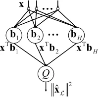
Each module in the ASSOM can be realized by a two-layer neural network [2], as shown in Fig. 1. Supposing a subspaceLis spanned by a set of basis vectors {b1,b2, . . . ,bH}, where H is the dimension ofL, the h-th neuron in the first layer take the orthogonal projectionxTbh ofx on bh, where 1≤h≤H. The basis vectors are supposed to be orthonormalized. The only quadratic neuron of the second layer sums up the squared outputs of the first-layer neurons. The output of the module is thenkxˆLk2, with ˆxLbeing the orthogonal projection of

xonL. It can be regarded as a measure of the matching betweenx andL. The input to an ASSOM network is typically an episode, i.e. a sequence of pattern vectors supposed to approximately span some linear subspace. Typi-cal examples of episodes used in the literature include sequences of temporally consecutive speech signals, transformations of image patchs. These vectors shall also be referred to as component vectors of the episode in this paper. By learn-ing the episode as a whole, the ASSOM is able to capture the transformation coded in the episode. For an input episode X = {x(s), s ∈ S}, where S is the index set of vectors in the episode, Kohonen proposed to use the energy

m(X,L) =P

s∈SkxˆL(s)k

2 _{as the measure of matching betweenXandL[2].}

1

b

b

b

Q

x

1 T

_b

x

2

ˆ

x

_b

x

x

b

Fig. 1.A module of the ASSOM realized as a neural network

2.2 ASSOM Learning Process

The learning process of ASSOM approximately minimizes the average projection error of input vectors in an iterative way. In each learning iteration, there are two basic stages: 1) Competition of the modules for an input episode; 2) Updating of the winner and its neighbors towards the input in a weighted fashion. A detailed account of the learning process at each iteration steptis as follows:

1. For the current input episodeX={x(s),s∈S}, locate the winning module

2. For each module i in the neighborhood of c, including c itself, update the subspaceLifor each component vectorx(s),s∈S, that is, update the basis vectorsb(_hi), according to the following rules:

(a) Rotateb(_hi)according to:

b(_hi)=

I+λ(t)h(i)

c (t)

x(s)xT(s) kxˆLi(s)kkx(s)k

b0_h(i) , (1)

whereb(_hi) is the new basis vector andb0_h(i)the old one.Iis the identity matrix, λ(t) a learning-rate factor that diminishes with t. h(ci)(t) is a neighborhood function defined on the ASSOM lattice.

(b) Dissipate the basis vectorsb(_hi), i.e. discard very small “noisy” compo-nents of the basis vectors, to force the basis vectors to learn the stronger and more fundamental features [2]. Orthonormalize these basis vectors afterwards.

A naive implementation of (1) requires a matrix multiplication which needs not only a large amount of memory, but also a computational load quadratic to the input dimension. In fact the formula (1) can be further simplified. It is not hard to get the following alternative formula:

b_h(i)=b_h0(i)+∆b(_hi) , (2)

where

∆b(_hi)=αc,h(i)(s, t)x(s) (3)

withα(c,hi)(s, t) being a scalar value defined by:

α(_c,hi)(s, t) =λ(t)h(i)

c (t)

xT(s)b0_h(i) kxˆLi(s)kkx(s)k

. (4)

This shows that the correction∆b(_hi) is in fact a scaling of the component vectorx(s), as illustrated in Fig. 2. After updating,b(_hi)represents betterx(s). Careful examination of (3) would reveal similarity of this formula with a recursive PCA suggested in [14]. The main difference is that here the gain of stochastic ap-proximation is modulated by a neighborhood function dependent on the module competition. Note that the computation of xT(s)b0_h(i) in (4) can be saved since it was computed when calculating the projectionkˆxLi(s)k(cf. Fig. 1). If we

cal-culate the scaling factorα(c,hi)(s, t) first, and then use it to scale the component vectorx(s), the basis vector updating speed can be dramatically improved.

2.3 A Deficiency of the ASSOM

) (i

h

b

( ' i

h

b

)

(

)

,

(

) (

, ) (

s

t

s

h c i

h

x

b

=

α

∆

)

(s

x

Fig. 2.An insightful view of the basis vector updating rule of ASSOM

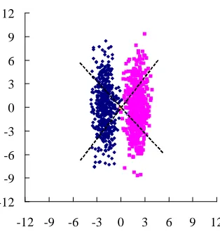
of this problem is the two clusters shown in Fig. 3. The basic ASSOM is unable to separate these two clusters. For a network of two modules with 1-D subspaces, each module learned one of the two basis vectors marked by the two dotted lines in the graph. This is also a difficult case for PCA since the first principal component will point to the vertical direction. However if we can also learn the offsets of the clusters, then theoretically the learning would be more accurate and consequently the two clusters can be separated properly. There has been some work in this direction in the literature. In the next section, we shall review some of this work.

-12 -9 -6 -3 0 3 6 9 12

-12 -9 -6 -3 0 3 6 9 12

3

Learning Linear Manifolds with the AOSSOM

The PCASOM and the AMSOM were proposed to improve the ASSOM so that the map can learn linear manifolds which do not necessarily pass through the origin. However the PCASOM is computationally expensive due to the covari-ance matrices to update and the eigenproblem to solve at each learning step. The AMSOM [9] is a direct extension of the ASSOM by appending a mean vectorm to each learned subspace. At each learning step,mis first updated according to the input vector by using an SOM training rule. Then the AMSOM shifts the manifold to the origin and updates the basis vectors in the same way as the AS-SOM does. Liu did not provide an objective error function in [9]. Minimization of the projection error by AMSOM is still to be theoretically justified. Contrary to the AMSOM, the AOSSOM proposed in this paper starts from an objective function, which is the average projection error. The algorithm is derived by min-imizing this error function in a gradient-descent manner. Convergence of the algorithm will at least guarantee a local minimum of the error function.

3.1 Projection Error Minimization by Gradient Descent

Each moduleiof an AOSSOM represents a linear manifoldAi described by an offset vectorr(i)_{and a set of basis vectorsb}(i)

h ,h= 1, . . . , H. It is not necessary for the offset vector to be the mean vector of the samples lying inAi. An error function is defined for the learning procedure:

E= Z

X

i∈I h(i)

c d(X,Ai)P(X)dX , (5)

where P(X) is the distribution of the random episode X ={x(s);s ∈S}. c is the index of the module which winsX.h(ci)is a neighborhood function as in the basic ASSOM.d(X,Ai) is a measure of the distance fromX toAi and defined as the projection error ofXonAi:

d(X,Ai) = X

s∈S

kx(s)−xˆAi(s)k

2 _{. (6)}

In the basic ASSOM, Ai is a linear subspace and the orthogonal projection of x(s) onAi is simply

ˆ

xAi(s) =

H X

h=1

(xT(s)b_h(i))b(_hi) . (7)

While in the more general case whereAiis a linear manifold defined by an offset vectorr(i)_{and the basis{b}(i)

1 , . . . ,b (i)

H}, the projection is defined by:

ˆ

xAi(s) =r

(i)₊

H X

h=1

x0ATi(s)b

(i)

h

where

x0Ai(s) =x(s)−r

(i) _{. (9)}

The projection residual ofx(s) on the linear manifoldAiis therefore defined by

˜

xAi(s) =x(s)−ˆxAi(s) . (10)

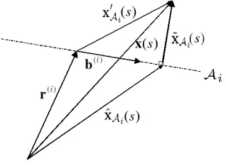
The relationship between parameters of the linear manifoldAi, x0Ai(s), ˆxAi(s)

and ˜xAi(s) is shown in Fig. 4 for the case whereAi is 1-dimensional.

Fig. 4. The relationship between parameters of the 1-D linear manifold Ai, x0Ai(s),

ˆ

xAi(s) and ˜xAi(s)

In (5), the indexcof the winning module depends on the input episodeXas well as on the status of all the modules in the network. The exact minimization of an objective function like (5) may be very complicated [2]. Instead, by using a stochastic approximation, we target the “sample” objective function at a certain learning step t based on the last input episode X and the last status of the network:

Es(t) =

X

i∈I

h(ci)(t)d(X,Ai) . (11)

The same strategy has been used to derive the basic ASSOM algorithm [2]. Taking gradients ofEs(t) with respect to the basis vectors, we have

∂Es

∂b(_hi)(t) =h

(i)

c (t)

∂d(X,Ai)

∂b(_hi) . (12)

This is all that we need for the basic ASSOM. Here for AOSSOM however we have the offset vector r(i) _{to update for each linear manifold A}

i. Thus we need an additional partial derivative forr(i)_:

∂Es

∂r(i)(t) =h (i)

c (t)

∂d(X,Ai)

∂r(i) . (13)

algebraic and calculus skills they are not hard to get. We suppose that the basis vectors are kept orthonormal in the gradient-descent process. Here are the results, for the offset vectorr(i)_,

∂Es

∂r(i)(t) =−2h (i)

c (t) X

s∈S ˜

xAi(s) , (14)

and for the basis vectors,

∂Es

∂b(_hi)(t) =−2h

(i)

c (t) X

s∈S

x0ATi(s)b

(i)

h

˜

xAi(s) . (15)

Taking a step length 1₂λb(t) in the opposite direction to the gradients for the basis vectors, whereλb(t) is a learning-rate factor for the basis vectors, the correction made to the basis vectors should be:

∆b(_hi)=hc(i)(t)λb(t) X

s∈S

x0ATi(s)b

(i)

h

˜

xAi(s) , (16)

and updating of the offset vectorr(i)_{would be:}

∆r(i)=hc(i)(t)λr(t) X

s∈S ˜

xAi(s) , (17)

whereλr(t) is the learning-rate factor for the offset vectorr(i)_.

Since ˜xAi(s)⊥b

(i)

h ,∀s, h, it is easy to show that

∆b(_hi)

1 ⊥b

(i)

h₂, ∀h1, h2 (18)

and ∆r(i)⊥b(_hi), ∀h . (19)

That is, updating of the linear manifoldAi is perpendicular to any current basis vector ofAi. This is also the steepest direction to updateAi towards the input. We remark that in the traditional ASSOM and in the AMSOM, the updating of the basis vectors has a redundant direction corresponding to the projection of the input vector on the (affine) subspace (cf. (3)). This might not be desirable since it would introduce instability to the basis vectors. Let us suppose that an input vectorx(s) lies perfectly in the (affine) subspace of the modulei. With the ASSOM and the AMSOM, the basis vectors are still updated as long asx(s) has a non-zero projection on the (affine) subspace. While with the AOSSOM, since the projection residual ˜xAi(s) is zero, the basis vectors remained unchanged,

which is a more desirable behavior.

3.2 AOSSOM Learning Process

1. For an input episode x(s),s∈S, locate the winning module indexed by

c= arg min i∈I

X

s∈S

k˜xAi(s)k

2 _{. (20)}

2. For each module i in the neighborhood of c, including c itself, update the linear manifoldAi, i.e. update the offset vector r(i) and basis vectors b(

i)

h for each component vectorx(s),s∈S. To updater(i), we use:

r(i)=r0(i)+∆r(i) , (21)

where∆r(i) is defined by (17). To updateb(_hi), we use

b_h(i)=b_h0(i)+∆b(_hi) , (22)

where∆b(_hi) is defined by (16). The basis vectorsb(_hi) are orthonormalized at the end of this step.

4

Cluster Separating Experiments

In this section, we demonstrate the capacity of the AOSSOM to learn and sepa-rate clusters which lie in linear manifolds away from the origin. For easier reading of this section, we first present some common parameters of the ASSOM, the AMSOM and the AOSSOM used in the following experiments. For each of the networks, the learning takes T = 10,000 steps. The neighborhood function is fixed to be Gaussian:

h(i)

c (t) = exp

−kuc−uik

2

2σ2_(t)

, (23)

where uc and ui are respectively the coordinates of the winning module c and the module i in the network lattice. σ(t) is related to the Full Width at Half Maximum (FWHM)w(t) byσ(t) =w(t)/2.3548. For all the networks through-out this section except the “AMSOM 1” in the third experiment,w(t) has the common form:

w(t) =w0

T

T+ 99t , (24)

wherew0should be set as such that the whole lattice can be properly covered at

the beginning of the learning procedure. The learning-rate parameters areλ(t) =

λ0T+99T tfor the ASSOM,λm(t) =λb(t) =λ0 T

T+99tfor the AMSOM, andλr(t) = λb(t) = λ_0T T

+99t for the AOSSOM.λm(t) is the learning-rate function for the mean vectors of the AMSOM. The initial learning rate λ0 shall be properly

4.1 First Experiment

In the first experiment, the goal is to learn the two Gaussian clusters in Fig. 3. The basic ASSOM is unable to learn the two clusters properly. Even with PCA, the first principal component would be directed to a vertical orientation, which does not give the best description of the two clusters and cannot separate them properly.

The settings of the first experiment are as follows. Each cluster in Fig. 3 is generated with a 2-D Gaussian distribution which shows an evident orientation, so that the cluster can be approximated by a 1-D linear manifold, which is a line, in the 2-D input space. 500 samples are generated for each cluster. We first show that the AOSSOM is able to learn the corresponding linear manifolds. Two modules are implemented in the AOSSOM network with each containing an offset vector and a basis vector. The initial learning rateλ0= 1. The learning results

are shown in Fig. 5. In the figure, the solid lines with arrows show the offset vectors learned by the AOSSOM. The dotted lines mark the 1-D linear manifolds learned by the AOSSOM. We can appreciate how well AOSSOM learned the two clusters and separated them by different offset vectors. Both modules found the linear manifolds which describe best the clusters in the sense of MSE (mean squared error).

-12 -9 -6 -3 0 3 6 9 12

-12 -9 -6 -3 0 3 6 9 12

Fig. 5.Result of learning two 1-D linear manifolds with the AOSSOM

After learning, each module was labeled with the cluster that it won for the most of the times. In testing, each input sample was assigned the label of the winning module. The experiments were repeated ten times for each network. In each repeat, 500 training samples and 500 test samples were randomly generated for each cluster and the networks were initialized randomly with different ran-dom seeds. The resulting classification accuracies are summarized in Table. 1. In the table, TR represents the training sets and TT the test sets. We can see that ASSOM works very poorly on such a distribution, it is practically a random predictor. Both AOSSOM and AMSOM can separate the two clusters with very high accuracies across different runs with various initializations of the networks.

Table 1. Classification accuracies for ten runs of the ASSOM, the AMSOM and the AOSSOM to separate the two Gaussian clusters in Fig. 5

n _{ASSOM AMSOM AOSSOM}

TR TT TR TT TR TT

1 50._{3% 52}._{3% 99}._{6% 99}._{9% 99}._{7% 99}._9% 2 51._{5% 51}._{3% 99}._{7% 99}._{8% 99}._{8% 99}._9% 3 51._{8% 50}._{9% 99}._{7% 99}._{9% 99}._{9% 99}._8% 4 52._{4% 50}._{3% 99}._{8% 99}._{9% 99}._{9% 99}._7% 5 51._{7% 50}._{9% 99}._{8% 99}._{8% 100% 99}._7% 6 51._{5% 51}._{4% 99}._{7% 99}._{9% 99}._{8% 99}._8% 7 51._{5% 51}._{4% 99}._{8% 99}._{8% 99}._{8% 99}._7% 8 50._{4% 50}._{1% 99}._{8% 100% 99}._{9% 100%} 9 53% 49._{8% 99}._{9% 99}._{8% 99}._{7% 100%} 10 50._{7% 52}._{2% 99}._{9% 99}._{8% 99}._{8% 99}._9%

4.2 Second Experiment

In the second experiment, the goal is to learn the three Gaussian clusters in Fig. 6. Each cluster is generated with a 2-D Gaussian distribution with one of the shown orientations, so that it can be approximated by a 1-D linear manifold. We intentionally introduced overlapping between different clusters to add to the difficulty of learning. 500 samples were generated for each cluster. We first show the capacity of the AOSSOM to learn the three linear manifolds. Three modules are implemented in the AOSSOM network with each containing an offset vector and a basis vector. As shown in Fig. 6, the AOSSOM learned the three clusters correctly despite the overlapping between clusters.

The basic ASSOM, the AMSOM and the AOSSOM are compared in terms of their ability to separate the three clusters. The experimental settings are the same as the previous experiment with two clusters except that here we use three modules in each network. λ0 = 1 was used for the ASSOM and the

-15 -12 -9 -6 -3 0 3 6 9 12 15

-15 -12 -9 -6 -3 0 3 6 9 12 15

Fig. 6. Result of learning three 1-D linear manifolds with the AOSSOM. The offset vector of the middle cluster is not plotted since it is too close to a zero vector

phenomena of the AMSOM whenλ0= 1. Even though the learning rate should

conventionally be in [0,1], as suggested by Liu [9], a larger starting learning rate seemed to have worked better for the AMSOM in this experiment. We will discuss this problem in the third experiment. For now we just choose the good parameters. The experiment was repeated ten times for each of the networks. 500 training samples and 500 test samples were randomly generated for each cluster at each run. The resulting classification accuracies are summarized in Table. 2. Due to overlapping between clusters, no classifiers can give perfect separation. The performance of the ASSOM is very poor for such a distribution. Both the AOSSOM and the AMSOM can separate these clusters with reasonably high accuracies across different runs with various initializations of the networks.

We may conclude that the AOSSOM is able to properly learn and separate clusters of these kinds, which are best described by distributions along linear manifolds shifted away from the origin. Such distributions cannot be adequately identified by linear subspaces used in the basic ASSOM.

4.3 Third Experiment

In the previous experiment we observed unstable phenomena of the AMSOM when λ0 = 1. A larger starting learning rate λ0 = 1.5 seemed to have worked

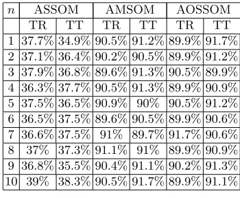
Table 2. Classification accuracies for ten runs of the ASSOM, the AMSOM and the AOSSOM to separate the three Gaussian clusters in Fig. 6

n _{ASSOM AMSOM AOSSOM}

TR TT TR TT TR TT

1 37._{7% 34}._{9% 90}._{5% 91}._{2% 89}._{9% 91}._7% 2 37._{1% 36}._{4% 90}._{2% 90}._{5% 89}._{9% 91}._2% 3 37._{9% 36}._{8% 89}._{6% 91}._{3% 90}._{5% 89}._9% 4 36._{3% 37}._{7% 90}._{5% 91}._{3% 89}._{9% 90}._9% 5 37._{5% 36}._{5% 90}._{9% 90% 90}._{5% 91}._2% 6 36._{5% 37}._{5% 89}._{6% 90}._{5% 89}._{9% 90}._6% 7 36._{6% 37}._{5% 91% 89}._{7% 91}._{7% 90}._6% 8 37% 37._{3% 91}._{1% 91% 89}._{9% 90}._9% 9 36._{8% 35}._{5% 90}._{4% 91}._{1% 90}._{2% 91}._3% 10 39% 38._{3% 90}._{5% 91}._{7% 89}._{9% 91}._1%

We randomly generated 10 different data sets. Each data set was composed of 4 clusters with 2-D Gaussian distributions. 500 training samples and 500 test samples were generated for each cluster. The mean vector of each cluster is random, with components in [−4,4] and a Euclidean norm not less than 2. Except the above settings, the clusters are allowed to have any amount of overlapping. So in general, they cannot be perfectly separated. Each AMSOM network as well as each AOSSOM network contains 4 modules. There is one basis vector in each module to simulate a 1-D linear manifold.

For the AMSOM, we experimented two configurations. In the first configura-tion, we used the exponential neighborhood-decreasing scheme suggested in [9]:

w(t) =w0exp(−

t

F) , (25)

where F is the learning step when w(F) = 0.368w0. In our experiments, we set

F = 5000. Changes toF did not show improved performance in our experiments.

w0 was set to 4 so that the full lattice could be covered at the beginning. The

initial learning rateλ0= 1. We did not observe improvement of the performance

with differentλ0in this experiment. The results we got on the first configuration

of the AMSOM are shown in Table 3 in the column “AMSOM 1”. In the table,D

is the serial number of the data sets generated. Different data sets have different four-cluster distributions. For a fair comparison, in the second configuration of the AMSOM, we chose the same neighborhood-decreasing function as that of the AOSSOM, which is shown in (24). The initial learning-rate was set to λ0 = 1.

Other values ofλ0 did not show improved performance in our experiments. The

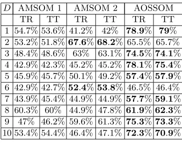
Table 3. Classification accuracies of the AMSOM and the AOSSOM for separating four Gaussian clusters. The boldface font emphasizes the best results at each run

D _{AMSOM 1 AMSOM 2 AOSSOM}

TR TT TR TT TR TT

1 54._{7% 53}._{6% 41}._{2% 42%} 78.9% 79% 2 53._{2% 51}._8%67.6%68.2% 65._{5% 65}._7% 3 48._{4% 48}._{6% 63% 63}._1% 74.5%74.1% 4 42._{9% 42}._{3% 45}._{2% 45}._2% 78.1%75.4% 5 45._{9% 45}._{7% 50}._{1% 49}._2% 57.4%57.9% 6 42._{9% 42}._7%52._4%53._{8% 46}._{5% 46}._4% 7 43._{9% 45}._{4% 44}._{9% 44}._{9% 57}._7%59._1% 8 60._{3% 60% 44}._{9% 47}._{8% 61}._9%62._3% 9 47% 46._{2% 59}._{6% 61}._{3% 75}._3%73._3% 10 53._{4% 54}._{4% 46}._{4% 47}._{1% 72}._3%70._9%

work the best, it still achieved a fairly good performance which is only at a little distance from the best.

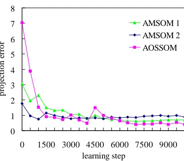
To see what happened when the AMSOM was trapped in a local minimum, we recorded the average projection errors on the test data set 1 in Table 3 with the AMSOM and the AOSSOM, which are shown in Fig. 7. As we can see from the figure, the “AMSOM 1” and the “AMSOM 2” converged to higher error levels than the AOSSOM. Higher error levels correspond to worse local minima. The “AMSOM 1” and the “AMSOM 2” seem to have stablized on the “bad” local minima and could not get out of them. In the process of convergence the AOSSOM also encountered a “bad” local minimum at aroundt= 4,000, where the error was 0.47. However it was able to get out of that “bad” local minimum and finally stablized at a better minimum, which was 0.40. In fact, even the “bad” local minimum 0.47 of the AOSSOM is already smaller than the converged local minima of the “AMSOM 1” and the “AMSOM 2”. The reason that the AOSSOM worked better than the AMSOM in most of the cases could be that the AOSSOM learning algorithm was derived from the gradient descent of the projection error function. Updating of the linear manifolds in a direction other than the negative gradient direction is more likely to be stuck in undesirable local minima.

5

Application of the AOSSOM to Handwritten Digit

Recognition

5.1 Related Work and Database

0 1 2 3 4 5 6 7 8

0 1500 3000 4500 6000 7500 9000 learning step

p

ro

je

ct

io

n

e

rr

o

r

AMSOM 1 AMSOM 2 AOSSOM

Fig. 7.Average projection errors of the first data set in Table 3 with the “AMSOM 1”, the “AMSOM 2” and the AOSSOM

basic ASSOM, they introduced nonlinearity to the hidden-layer neurons of the autoencoders. Their experiments showed impressive performance on a database of the U.S. National Institute of Standards and Technology (NIST), which con-sists of 20,000 numerals. In this section, we apply the AOSSOM, an alternative improvement of the basic ASSOM, to handwritten digit recognition.

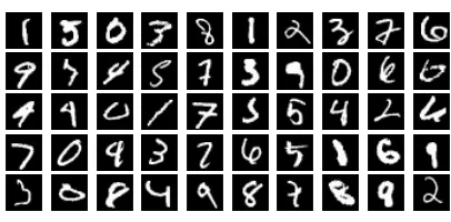
The handwritten digit image database used in this paper is a modified NIST (MNIST) database by mixing NIST’s datasets. The database is made publicly available by LeCunet al. [13]. Images in this database were size normalized and centered in a 28×28 pixel field. The resulting images contain gray levels as a result of the interpolation technique used by the normalization algorithm. The foreground is coded with high gray levels and the background with low gray levels. The database contains a training set of 60,000 digits and a test set of 10,000 digits. Some examples from this database are shown in Fig. 8. A large variety of writing styles are covered by the database as shown by these examples.

5.2 Learning Handwritten Digits with the AOSSOM

As an application of the AOSSOM, our handwritten digit recognition system is designed as follows. An AOSSOM network is trained for each class of examples. An input digit image is classified by examining which network gives the best reconstruction. Similar ideas were proposed in [15] and [7]. In [15], PCA and factor analysis (FA) were proposed as local models of handwritten digit image manifolds. In [7], ASSOM networks realized by non-linear autoencoders were implemented for the local modeling.

Fig. 8.Some examples from the MNIST handwritten digit image database

before entering the networks. The learning steps of each AOSSOM network is set to T = 30,000. The learning-rate factor has the formλr(t) =λb(t) = λ_0T T

+99t whereλ0was set to 1. The neighborhood function is Gaussian with the FWHM

w(t) = w0T+99T t where the initial value w0 depends on the network size. The trained AOSSOM networks of 5×5 modules with two basis vectors are shown in Fig. 9. Each module in thek-th networkMk, k= 0, . . . ,9, learned a linear manifold for the images of the digitk. Each manifold contains an offset vectorr and two basis vectorsb1andb2. These vectors are visualized by normalizing the

grayscales into [0,255]. For a mean-subtracted and normalized test input digit imagex, each networkMk gives a reconstruction vector ˆxMk. The class label of

xis determined by the network which gives the minimum reconstruction error:

k∗= arg min

k kx−xˆMkk . (26)

Now it comes to the question of how to build the reconstruction ˆxMk for

each network. The idea is to combine the set of reconstruction vectors ˆxAkifrom

the|Ik|modules in the networkMk, whereIk is the set of modules inMk and Aki the linear manifold learned by thei-th module inMk. The combination is a weighted average:

ˆ xMk=

P

i∈IkakixˆAki

P i∈Ikaki

. (27)

This weighted average was also used in [7]. There is no clear evidence that the choice of the weighting function is critical [16]. One choice is the Gaussian function which has infinite extent [7]:

aki= exp

−kx−xˆAkik

2

2σ2

ki

, (28)

x=

↓

M0 M1 M2 M3 M4

r

b1

b2

↓ ↓ ↓ ↓ ↓

ˆ

xMk

M5 M6 M7 M8 M9

r

b1

b2

↓ ↓ ↓ ↓ ↓

ˆ

xMk

Fig. 9.AOSSOM networks trained for the MNIST database. For a mean-subtracted and normalized test input digit imagex, each network builds a reconstruction vector ˆ

5.3 Experimental Results

We have experimented on different sizes of AOSSOM networks with different numbers of basis vectors in each module. The results are summarized in Table 4. The network lattices are squares with the dimension W varying from 3 to 8. Thus the number of modules in each network isW2_{. As we can see, in general, a}

larger network size leads to a better recognition accuracy. But this also increases the training and testing time. A higher manifold dimension can achieve a better performance, this is more evident when the network size is smaller. In general, this classification system exhibits a promising recognition performance on the handwritten digit images.

Table 4.Handwritten digit recognition accuracies of the AOSSOM network with dif-ferent lattice sizesW _{and linear manifold dimensions}H

W H_{= 1} H _{= 2} H_{= 3}

TR TT TR TT TR TT

3 94._{6% 94}._{7% 95}._{6% 95}._{6% 96}._{3% 96}._2% 4 95._{7% 95}._{7% 96}._{4% 96}._{3% 96}._{9% 96}._5% 5 96._{3% 96}._{2% 96}._{9% 96}._{7% 97}._{2% 96}._8% 6 96._{7% 96}._{3% 97}._{1% 96}._{8% 97}._{7% 97}._1% 7 97._{1% 96}._{6% 97}._{4% 96}._{9% 97}._{6% 96}._9% 8 97._{5% 97% 97}._{8% 97}._{1% 98% 97}._3%

Some of the correctly recognized digits are shown in Fig. 10. In the figure, the first column shows the input digit images. The other columns show the images reconstructed by the individual networks. The images are equalized to 255 gray levels. In the first column, numbers to the left of the arrows are the ture labels and numbers to the right are the labels assigned by the system. Numbers in the other columns are reconstruction errors of the individual networks. For each shown input digit image, the network corresponding to the correct digit label gives the best reconstruction, as confirmed by the output reconstruction errors. The other networks often output ambiguous reconstruction vectors, e.g. the output of the 4-th network for the input digit 2 and that of the 8-th network for the input digit 6. The written style of the input digit 9 is similar to 4, and this is confirmed by the output of the 4-th network, whose reconstruction error is close to that of the 9-th network.

Figure 11 shows some incorrectly classfied digits. Some of the input examples are really ambiguous, e.g. 4 → 9 and 9→ 1. We have observed in the experi-ments that the most probable errors come from 2→ 7, 4→ 9 and 6→0. By examining the output reconstruction errors, we can find that even though the recognition failed, the error of the true-class network could be very close to the minimum error. For example, in the false classification 9→1, the shown error of the network M1 is practically the same as that of M9. In fact, the errors

0→0 0.41 1.02 0.76 0.81 0.92 0.72 0.78 0.92 0.78 0.91

2→2 0.92 0.88 0.62 0.85 0.91 0.92 0.85 0.92 0.88 0.94

4→4 0.91 0.96 0.86 0.84 0.51 0.81 0.84 0.73 0.79 0.71

6→6 0.83 0.99 0.90 0.94 0.90 0.90 0.64 0.98 0.90 0.95

8→8 0.79 0.89 0.65 0.76 0.78 0.76 0.78 0.81 0.60 0.76

9→9 0.83 0.77 0.78 0.68 0.52 0.73 0.85 0.66 0.61 0.48

Fig. 10.Some digits correctly recognized by the AOSSOM networks

is effectively 0.4637 and that from M9 is 0.4639. The difference is practically

negligible here. Better accuracies could be achieved by rejecting some input in-stances when the smallest reconstruction error and the second smallest are very close.

6

Conclusions and Perspectives

In this paper, the AOSSOM, an improvement of the basic ASSOM, was pro-posed. It is able to learn a set of ordered linear manifolds. The AOSSOM works by minimizing a projection error function in a gradient-descent manner. We demonstrated by experiments that the AOSSOM is able to learn linear manifolds of clusters shifted away from the origin and separate the clusters accordingly. The basic ASSOM cannot identify clusters of such kinds adequately. The AOS-SOM is more robust to local minima than the AMAOS-SOM as revealed by the cluster separating experiments. The reason could be that the updating of the manifolds follows the negative gradient direction. Other directions, such as the one used in the AMSOM, could be more prone to local minima. The proposed network was then applied to handwritten digit recognition and showed promising results.

0→6 0.77 1.04 0.83 0.90 0.88 0.89 0.74 0.88 0.95 0.87

2→7 0.94 0.72 0.62 0.74 0.78 0.86 0.98 0.56 0.70 0.73

4→9 0.92 0.82 0.84 0.77 0.56 0.76 0.92 0.66 0.76 0.51

6→0 0.72 1.08 0.91 0.88 0.94 0.85 0.78 0.86 0.92 0.95

7→9 0.76 0.98 0.75 0.84 0.82 0.86 0.90 0.62 0.80 0.61

9→1 0.87 0.46 0.79 0.65 0.56 0.69 0.83 0.62 0.62 0.46

Fig. 11.Some digits incorrectly recognized by the AOSSOM networks

References

1. Kohonen, T.: The Adaptive-Subspace SOM (ASSOM) and its use for the imple-mentation of invariant feature detection. In Fogelman-Souli´e, F., Gallinari, P., eds.: Proc. ICANN’95, Int. Conf. on Artificial Neural Networks. Volume 1., Paris (1995) 3–10

2. Kohonen, T., Kaski, S., Lappalainen, H.: Self-organized formation of various invariant-feature filters in the Adaptive-Subspace SOM. Neural Computation9(6) (1997) 1321–1344

3. Oja, E.: Principal components, minor components, and linear neural networks. Neural Networks5(6) (1992) 927–935

4. Hase, H., Matsuyama, H., Tokutaka, H., Kishida, S.: Speech signal processing using Adaptive Subspace SOM (ASSOM). Technical Report NC95-140, The Inst. of Elec-tronics, Information and Communication Engineers, Tottori University, Koyama, Japan (1996)

5. Ruiz-del-Solar, J.: TEXSOM: Texture segmentation using Self-Organizing Maps. Neurocomputing21(1-3) (1998) 7–18

6. de Ridder, D., Lemmers, O., Duin, R.P.W., Kittler, J.: The Adaptive Subspace Map for image description and image database retrieval. In: SSPR/SPR. (2000) 94–103

7. Zhang, B., Fu, M., Yan, H., Jabri, M.: Handwritten digit recognition by Adaptive-Subspace Self-Organizing Map (ASSOM). IEEE Trans. Neural Networks 10(4) (1999) 939–945

8. L´opez-Rubio, E., Mu˜noz-P´erez, J., G´omez-Ruiz, J.A.: A Principal Components Analysis Self-Organizing Map. Neural Networks17(2) (2004) 261–270

10. Kawano, H., Horio, K., Yamakawa, T.: Adaptive Affine Subspace Self-organizing Map with kernel method. In Pal, N.R., Kasabov, N., Mudi, R.K., Pal, S., Parui, S.K., eds.: Proc. 11th Int. Conf. on Neural Information Processing. Volume 3316 of Lecture Notes in Computer Science., Calcutta, India, Springer (2004) 387–392 11. L´opez-Rubio, E., Mu˜noz-P´erez, J., G´omez-Ruiz, J.A., Dom´ınguez-Merino, E.: New

learning rules for the ASSOM network. Neural Comput & Applic 12(2) (2003) 109–118

12. Suen, C.Y., Nadal, C., Legault, R., Mai, T.A., Lam, L.: Computer recognition of unconstrained handwritten numerals. Proc. IEEE 80(7) (1992) 1162–1180 13. Lecun, Y., Bottou, L., Bengio, Y., Haffner, P.: Gradient-based learning applied to

document recognition. Proc. IEEE86(11) (1998) 2278–2324

14. Oja, E.: Subspace Methods of Pattern Recognition. Research Studies Press, Letch-worth, UK (1983)

15. Hinton, G.E., Dayan, P., Revow, M.: Modeling the manifolds of images of hand-written digits. IEEE Trans. Neural Networks8(1) (1997) 65–74