warwick.ac.uk/lib-publications
Original citation:
Sawlekar, Rucha, Montefusco, Francesco, Kulkarni, Vishwesh V. and Bates, Declan G.. (2016)
Implementing nonlinear feedback controllers using DNA strand displacement reactions. IEEE
Transactions on NanoBioscience .
Permanent WRAP URL:
http://wrap.warwick.ac.uk/79400
Copyright and reuse:
The Warwick Research Archive Portal (WRAP) makes this work by researchers of the
University of Warwick available open access under the following conditions. Copyright ©
and all moral rights to the version of the paper presented here belong to the individual
author(s) and/or other copyright owners. To the extent reasonable and practicable the
material made available in WRAP has been checked for eligibility before being made
available.
Copies of full items can be used for personal research or study, educational, or not-for profit
purposes without prior permission or charge. Provided that the authors, title and full
bibliographic details are credited, a hyperlink and/or URL is given for the original metadata
page and the content is not changed in any way.
Publisher’s statement:
© 2016 IEEE. Personal use of this material is permitted. Permission from IEEE must be
obtained for all other uses, in any current or future media, including reprinting
/republishing this material for advertising or promotional purposes, creating new collective
works, for resale or redistribution to servers or lists, or reuse of any copyrighted component
of this work in other works.
A note on versions:
The version presented here may differ from the published version or, version of record, if
you wish to cite this item you are advised to consult the publisher’s version. Please see the
‘permanent WRAP url’ above for details on accessing the published version and note that
access may require a subscription.
Implementing Nonlinear Feedback Controllers using
DNA Strand Displacement Reactions
Rucha Sawlekar
1, Francesco Montefusco
2, Vishwesh V. Kulkarni
1and Declan G. Bates
1Abstract—We show how an important class of nonlinear feedback controllers can be designed using idealized abstract chemical reactions and implemented via DNA strand displace-ment (DSD) reactions. Exploiting chemical reaction networks
(CRNs) as a programming language for the design of complex circuits and networks, we show how a set of unimolecular and bimolecular reactions can be used to realize input-output dynam-ics that produce a nonlinearquasi sliding mode(QSM) feedback controller. The kinetics of the required chemical reactions can then be implemented as enzyme-free, enthalpy/entropy driven DNA reactions using a toehold mediated strand displacement mechanism via Watson-Crick base pairing and branch migration. We demonstrate that the closed loop response of the nonlinear QSM controller outperforms a traditional linear controller by facilitating much faster tracking response dynamics without introducing overshoots in the transient response. The resulting controller is highly modular and is less affected by retroactivity effects than standard linear designs.
Index Terms—Sliding mode control, DNA strand displacement, chemical reaction networks, saturation nonlinearity, retroactivity.
I. INTRODUCTION
S
EVERAL of the proposed industrial and biomedical appli-cations of synthetic biology require the ability to precisely and robustly control the behaviour of synthetic circuits or devices at a biomolecular level [1], [2]. A fundamental aim of synthetic biology is thus to achieve the capability to design and implement robust embedded biomolecular feedback control circuits [3]. One appropriate modelling and design framework for tackling this problem is provided by chemical reactionnetworks (CRNs), which represent a convenient and concise
approach to modelling chemical and biological processes, as well as an effective tool for the analysis of their behaviour from both deterministic [4], [5] and stochastic [6], [7] view-points. Previous work on the implementation of feedback controllers using DNA within this framework has focussed on the design of linear time-invariant systems only, e.g. the
proportional+integrator (PI) controllers described in [8], [9], [10]. This approach fails to exploit the inherent potential of biomolecular circuits to implement nonlinear dynamical systems [11], [12], [13], and also requires the use of additional circuitry to overcome the wind-up effects associated with the integrator action.
1Rucha Sawlekar, Vishwesh Kulkarni and Declan Bates are with
the Warwick Centre for Integrative Synthetic Biology (WISB), School of Engineering, University of Warwick, Coventry, CV4 7AL, United Kingdom e-mail: [email protected], [email protected], [email protected].
2Francesco Montefusco is with the Department of Information Engineering,
University of Padova, Padova 35131 e-mail: [email protected].
In this paper, we extend the approach of [8], [9], [10] to allow the implementation of nonlinear feedback controllers. We focus on a well-known type of nonlinear controller called
a sliding mode controller(SMC), whose strong performance
and robustness characteristics have been widely recognised in more traditional control engineering applications [14], [15]. From sliding mode control theory, a perfect SMC can be represented by a relay nonlinearity (see [14], [16], [17]). To avoid a number of theoretical and practical issues with the implementation of such discontinuous switches, in engineering practice SMC’s are usually implemented as quasi sliding mode (QSM) controllers, i.e. continuous/smooth approxima-tions of the discontinuous SMC. Here, we show how a set of irreversible chemical reactions can provide a biomolecular implementation of a nonlinear QSM controller. We show how the kinetics of the required chemical reactions can then be implemented as enzyme-free, entropy/enthalpy driven DNA reactions [18], using strand displacement as an elementary computational mechanism.
We implement this controller on a prototype embedded closed loop feedback system that consists of three individual modules, a subtractor, a controller and a biomolecular process to be controlled, each realized by mass action kinetics at a molecular level and interconnected using a modular approach as shown in Fig. 1. In contrast to previous implementations of DNA-based feedback controllers, the biomolecular process to be controlled here is both dynamic and nonlinear. Note also that the subtractor module must be represented as a dynamical system, unlike in standard feedback control systems which assume the availability of an ideal subtractor. Analysis of the closed loop performance of the QSM controller reveals significant performance advantages compared to a linear PI controller, particularly when retroactivity effects (see [19], [20], and [21]) are taken into account.
OR
KP
KI +
QSM
Controller PI Controller
Subtractor Process
Reference Input U
Feedback Signal Y
Output Y Error X1
Controller Output A
KP
[image:3.612.100.518.54.147.2]KI +
Fig. 1: A prototype embedded biomolecular closed loop feedback control system
II. RECENTWORK
Our notation follows that used in [8] and [9]: for exam-ple, we represent a bidirectional, i.e. reversible, bimolecular chemical reaction as:
X1+X2 k1
−* )− k2
X3+X4,
where, Xi are chemical species with X1 and X2 being the
reactants and X3 andX4 being the products. Here,k1denotes
the forward reaction rate and k2 denotes the backward
reac-tion rate. A unimolecular reacreac-tion features only one reactant whereas a multimolecular reaction features two or more re-actants. Degradation of a chemical species X at ratek into a waste product or an inert form is denoted as X−→k /0.
A. DNA strand displacement mechanism
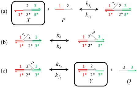
We now present a brief overview of the DNA Strand Displacement (DSD) mechanism (see [23] and [24]) through which the types of idealized chemical reactions used in this paper may be implemented. Consider the reversible bimolec-ular reaction:
X+P−)−k−*b− kub
Y+Q, (1)
where, X, P, Y and Q are DNA strands while kb and kub
are the binding and unbinding rates, respectively. A DSD
Fig. 2: Examples of DNA strand displacement reactions illus-trated using the software package Visual DSD [25] : the DNA strands are bonded by Watson-Crick base pairing, denoted by∗ and the basic steps involved are (a) binding of toehold1to1*, (b) branch migration wherein the strand1-2partially displaces strand2-3, and (c) complete separation of strand 2-3[26].
implementation of this reaction is shown in Fig. 2. It begins with an invader strandPbinding to the complementary target strandX at the toehold1*through Watson-Crick base pairing [27]. Through an intermediate process ofbranch migration,P
displaces the evader strand2-3fromX, thereby producing the partially double stranded productY that can further react with other DNA complexes using the toehold3*.
If DNA strands belong to entirely different domains, as is often the case, they do not interact with each other directly and therefore DSD reactions must be mediated by so-called auxiliary DNA species, which must be present in sufficiently large amounts [26]. We assume that complementary strands react only with each other, although this constraint can be relaxed, as demonstrated in [10]. For the DSD reactions to be fast and thereby reduce mismatches during branch migrations, the toehold domains should be short: for example, of the order of 6–10 nt, wherentdenotes nucleotides, and the displacement domains should preferably be 20 nt [28]. The reaction rate constants, and consequently the kinetics of the system, are a function of the toehold binding strength and can thus be altered by varying the binding strength and the strand composition [26]. Elementary DNA reactions are approximated into CRNs by excluding auxiliary species as described in [11] (see Ap-pendix). Corresponding reaction rates are also approximated in terms of initial concentration of auxiliary DNA species (Cmax),
and forward binding reaction rates (qi andqmax).
B. Representing linear systems using idealized chemical reac-tions
Linear time-invariant (LTI) systems can be realized using three types of operations: integration, summation, and multi-plication by a constant. Here we summarise previous results on how such systems can be realized using idealized chemical reactions.
Whereas signals in systems theory can take both positive and negative values, biomolecular concentrations can only take non-negative values. To resolve this difficulty, we follow the approach in [8] and [9], and represent a signal x as the difference in concentrations of two DNA strands. Here, x+
[image:3.612.62.286.521.665.2]0 20,000 40,000 0
5 10 15 20
Simulated trajectories
Time (sec) x+
x−
0 20,000 40,000
−10 −5 0 5 10
[image:4.612.56.299.52.188.2]x
Fig. 3: The square wave signal (right) is generated by two instantaneous additions of chemical species att=0, 20,000s using the relationx(t) =x+(t)−x−(t). DNA strandx+is added at timet=0 withx−being absent (left) resulting in a positive value of the signalxfort∈[0,20,000)s. Later, DNA strandx−
is added at timet=20,000s resulting in the signalxbecoming negative for t∈[20,000,40,000)s.
In [8], results on how to represent elementary system theoretic operations such as gain, summation and integration using idealized abstract chemical reactions were obtained and it is shown that only three types of elementary chemical reactions, namely, catalysis, annihilation and degradation are needed for such representations. In [9], this set of elementary chemical reactions was further reduced to only two. We now summarise the main results and refer the interested reader to [8] and [9] for the complete background theory.
Strictly speaking, each of the below equations with super-script ± and ∓ should be written down after decomposing them into their ‘+’ and ‘−’ individual components - for example,x±i −→k x±o should be written as the set of the following
two reactions: x+i −→k x+o andx−i −→k x−o. However, for brevity, following [8], we will represent such a set of reactions compactly as x±i −→k x±o.
Lemma 1:[Scalar gain K]
Let xo=Kxi wherexi is the input, xois the output and K is
the gain. This operation is implemented using the following
set of abstract chemical reactions:x±i −→γK x±i +x±o,x±o −→γ /0 and
x+o +x−o −→η /0, whereγ andη are the kinetic rates associated with degradation and annihilation respectively.
Lemma 2:[Summation]
Consider the summation operation xo=xi+xd, where xi and xdare the inputs andxois the output. This operation is
imple-mented using the following set of abstract chemical reactions:
x±i −→γ x±i +x±o,x±d −→γ x±d +x±o,x±o −→γ /0 andx+o +x−o −→η /0. The subtraction operation xo=xi−xd is implemented using the
following set of abstract chemical reactions: x±i −→γ x±i +x±o,
x±d −→γ x±d+xo∓,xo±−→γ /0 andx+o+x−o −→η /0.
Lemma 3:[Integration]
Consider the integrator xo=K R
xidt where, xi is the input, xo is the output, and K is the DC gain. This operation is
implemented using the following set of abstract chemical reactions: x±i −→K x±i +xo± andxo++x−o −→η /0.
Using generalised mass-action kinetics, it follows that the
gain operator realized in this manner is described using the ODE, dxo
dt =γ(Kxi−xo). Likewise, the ODEs for the
summa-tion and integrator operasumma-tions are given by dxo
dt =γ(xi+xd−xo)
and dxo
dt =Kxi, respectively.
III. MAINRESULTS
We now present our main results on how the closed loop system modules shown in Fig. 1 can be synthesized individu-ally using DNA strand displacement reactions.
A. Quasi sliding mode controller
Taking inspiration from the ultrasensitive input-output behaviour exhibited by mitogen-activated protein kinases
(MAPK) signaling cascades, [29], [30], [31], we now present a set of idealized chemical reactions that can be used to gen-erate switch-like input-output responses. When implemented as elementary DNA reactions, for example by using the software package Visual DSD [25], these reactions can be used to construct a nonlinear QSM feedback controller. Consider the following set of idealized CRNs, where the signal X1
is the input of the system and the signal A is the output,
X1=X1+−X1−andA=A+−A−, respectively, and the strands
X1+,X1− andA+,A− have a free toehold each:
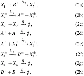
X1±+B±−k−b1→X2±, (2a)
X2±−k−c1→A±+X1±, (2b)
X2++X2−−→η φ, (2c)
A++A−−→η φ, (2d)
A±+X3±−k−b2→X4±, (2e)
X4±−k−c2→B±+X3±, (2f)
X4++X4−−→η φ, (2g)
B++B−−→η φ. (2h)
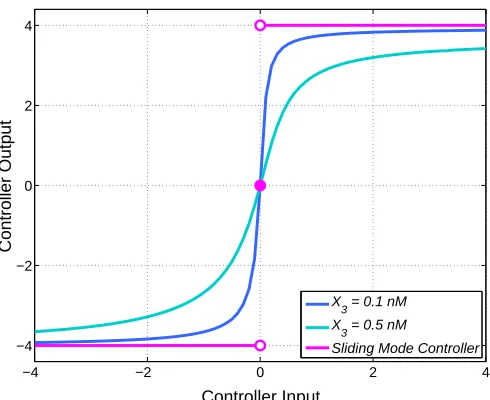
The above CRNs realize an ultrasensitive switch-like input-output response, as illustrated in Fig. 4. By tuning the con-centration of the DNA strandsX3±, the input-output response of the set of CRNs can be made to closely approximate the ideal switch implemented by a SMC, i.e. the set of CRNs (2) implements a QSM controller. Here, kb1 and kb2 denote the binding reaction rates whereaskc1 andkc2 denote the catalytic reaction rates.
[image:4.612.400.564.355.504.2]The CRNs (2) are approximations of elementary DNA reac-tions which can be realized using Visual DSD software, [25], as illustrated in Figs. 5, 6 and 9. The DSD implementation of the catalysis reactions given by (2b) and (2f) is shown in Fig. 5. Accordingly, the reactions (2b), (2f) initiate with the
single strand DNA(ssDNA) X2±(or X4±) displacing auxiliary species G±i irreversibly at the rate qi, producing the
interme-diate complex O±i and waste. Complex O±i on reacting with auxiliary species Ti±, releases two single stranded products,
−4 −2 0 2 4 −4
−2 0 2 4
Controller Input
Controller Output
X
3 = 0.1 nM
X
3 = 0.5 nM
[image:5.612.52.297.64.264.2]Sliding Mode Controller
Fig. 4: Input-output characteristics of an ideal sliding mode controller and quasi sliding mode controller for different values of the tuning parameter X3.
the reaction begins with single strand X1± (or A±) reacting reversibly with the auxiliary species L±i to produce activated intermediate complexes Hi± andB±i . Due to the presence of
X1± (or X3±) in the solution with an active toehold, it reacts with complexHi±to release intermediate complexO±i . IfX1±
is absent then B±i can reversibly displace Hi±, releasing X1±
back into the solution. ComplexO±i displacesTi±. Hence, the bimolecular reactions given by (2a) and (2e) are irreversible and produce ssDNA products X2± andX4±, respectively. The full set of elementary DNA reactions required to realize the QSM controller are given in the appendix.
Now, using mass action kinetics, the set of reactions given by (2) may be represented by the following set of ODEs:
dA
dt =kc1X2−kb2AX3, (3a)
dX2
dt =kb1X1B−kc1X2, (3b)
dB
dt =−kb1X1B+kc2X4, (3c)
dX4
dt =kb2AX3−kc2X4. (3d)
where, X1 is the input and A is the output of the QSM
controller. From equations (3a) to (3d) we can see that A+
B+X2+X4=constant
.
=Sqsm. Thus the signal B is variable
and depends on the dynamic signals A,X2,X4. Since,X1 also
varies over time this means that the term kb1X1B in (3b) is nonlinear. It can be checked that:
dX2+
dt = kb1X
+
1B
+−k c1X
+
2 −ηX
+
2X
−
2, (4)
dX2−
dt = kb1X
−
1B
−−k
c1X
−
2 −ηX2+X
−
2. (5)
Hence,
dX2
dt =
dX2+
dt −
dX2− dt
= (kb1X
+
1B
+−k c1X
+
2 −ηX
+
2X
−
2)
−(kb1X
−
1B
−−
kc1X
−
2 −ηX
+
2X
−
2 )
= kb1{(X
+
1B
+)−(X−
1B
−)} −k
c1(X
+
2 −X
−
2)
= kb1{(X1B)+−(X1B)−)} −kc1X2,
where,X1+B+= (X1B)+andX1−B−= (X1B)−. Hence,
dX2
dt = kb1X1B−kc1X2.
Now, from sliding mode control theory, a perfect SMC can be represented by a relay nonlinearity (see [14], [16], [17]). As shown in Fig. 4, this can be obtained as the limiting case of a controller implemented using the equations (3a) - (3d). For example, asX3→0, the outputAof the controller can be
described by the following relay-type saturation nonlinearity (see Fig. 4):
A(t) =kSMC ·sgn(X1(t)), (6)
where sgn(·) denotes the signum function and X1(t) is the
input to the controller (the error signal generated by the sub-tractor). Such a controller has a discontinuity on the straight line X1=0 which is traditionally referred to as the sliding
manifold σ de f= X1=0, where σ is the sliding variable. The control signalA, defined by (6), is therefore designed to force the system to move toward the sliding manifold σ =0 (the
reaching phaseof SMC) and then maintain this condition (i.e.
σ=0) for all future time (the sliding phaseof SMC). In practice, however, implementations of perfect sliding mode controllers cause the system’s closed loop response to exhibit a zigzag motion of small amplitude and high frequency, due to imperfections in switching devices and delays [14], [16], [17]. This effect, known as chattering, is typically avoided by using continuous/smooth approximations of the discontinuous SMC, resulting in a so-calledquasi sliding mode
(QSM) controller.
The controller implemented using equations (3a) - (3d) is an example of such a function, since it approximates the nonlinearity sgn(X1). Since with a QSM controller there is
no ideal sliding mode in the closed loop system, the sliding variable (error) cannot be driven exactly to zero in a finite time, [14]. However, if our QSM controller is made more ultrasensitive (for example, by decreasingX3), the input-output
behaviour of our QSM controller approaches the limiting case of an ideal SMC, as illustrated in Fig. 4, and the error signal can be made as small as desired.
B. Nonlinear process to be controlled
bimolec-DNA Implementation CRNs
X1±+G±i −→qi φ+O±i (7)
O±i +T±i −−→qmax X±2 +X±3 (8) X±1 −k1→X±2 +X±3 (9)
where, qi=
k1
[image:6.612.54.563.49.190.2]Cmax
Fig. 5: Catalysis reactionX1±→X2±+X3±. The DNA implementation with reaction index icorresponding to the unimolecular CRN using signal species X1±,X2±andX3±highlighted in black boxes. Domain 1∗qmay not be entirely complement of domain
1 but its toehold domain reaction rate is tuned toqi. In (16), speciesGireacts withX to displaceOiand in (17),OireleasesX
andY, on reacting with speciesTi [11]. The question mark appearing on the DNA strands such asX1andφ, indicates species identifier; as adapted from [8].
DNA Implementation CRNs
X±1+L±i −−)qi−−*
qmax H
±
i +B±i (10)
X±2+H±i −−→qmax O±i +φ (11)
O±i +T±i −−→qmax X±3 (12) X±1 +X±2 −k2→X±3 (13)
where, k2=qi
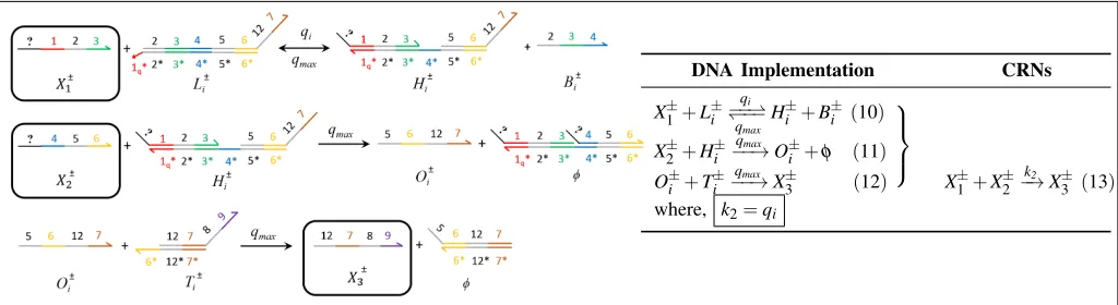
Fig. 6: Bimolecular CRN X1±+X2±−→k2 X3±: DNA implementation of bimolecular CRN (13) with reaction index i and black boxes highlighting the formal species, X1±, X2±, X3± that appear in the approximated CRN. In (10) X1± displaces auxiliary species L±i reversibly producing intermediate complexHi±which reacts with X2±as given in (11) producingO±i . In (12), X3±
is produced when O±i irreversibly displaces Ti±; as adapted from [11].
ular reactions, given as follows, whose dynamics are to be controlled:
A±+X5±−→kr1 X6±, (14a)
X6±−→kr2 Y±+X5±, (14b)
Y±−→kr3 φ, (14c)
Y++Y−−→η φ. (14d)
Here, the process input is the ssDNA A± and the process output is the ssDNA Y±. kr1 is a binding reaction rate, kr2 is the catalytic reaction rate, and kr3 is the degradation rate. These reaction rates and their values are as listed in Table II.
This process was chosen because application of standard Michaelis-Mentens kinetics to these reactions results in a set
of ODEs with nonlinear response dynamics, given by:
dX5
dt =−kr1AX5+kr2X6, (15a)
dX6
dt =kr1AX5−kr2X6, (15b)
dY
dt =kr2X6−kr3Y. (15c)
From (15), we can conclude that XTotal =. X5+X6 is
con-served through the lifetime of the process and have therefore set it to a constant value, as noted in Table II. In the context of our feedback system shown in Fig. 1, the process input signal is the controller outputAand the process output signal
[image:6.612.52.564.269.409.2]DNA Implementation CRNs
X±+G±i −qi→φ+O±i (16)
O±i +T±i −−→qmax X±+Y± (17) X±−k3→X±+Y± (18)
where, qi=
k3
[image:7.612.48.562.49.190.2]Cmax
Fig. 7: Catalysis reactionX±→X±+Y±. The unimolecular catalysis CRN (18) is approximated from the DNA implementation with reaction index i. The signal species areX± andY±. In (16), species Gi±reacts withX± to produceO±i and in (17),O±i
releases X± andY±, on reacting with speciesTi±; as adapted from [8]. The strand displacement mechanism resembles that in Fig. 5 but, the nucleotide composition of product species vary depending on the composition of auxiliary species involved [11].
DNA Implementation CRNs
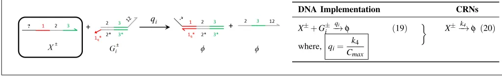
X±+G±i −→qi φ (19) X±−k4→φ (20)
where, qi=
k4
Cmax
Fig. 8: Degradation reaction X±−k→4 φ: DNA implementation of formal species X± degradation on reacting with auxiliary species Gi. In (19), X± performs strand displacement onGi producing inert waste. (20) represents the CRN derived from the
formal DNA strand displacement reaction (19); as adapted from [8].
represents the first attempt to design a feedback controller for a biomolecular process which is both dynamic and nonlinear.
C. Subtractor
Following [8] and [10], we implement the subtractionU−Y
of two signals U and Y. The subtraction operation can be achieved using the following set of reactions:
U±−k→s U±+X1±, (21a)
Y±−k→s Y±+X1∓, (21b)
X1±−k→s φ, (21c)
X1++X1−−→η φ. (21d)
Here, signalsU andY are the inputs andX1 is the output
of the subtractor. In other words, the value of signalX1being
produced is equivalent to that of the difference between the two input signals, U and Y. In addition, both the catalysis reaction rates in (21a)-(21b) are set to be equal to the degradation rate. Note that this subtractor module is itself a dynamical system and produces the desired result, i.e., subtraction of the two input signals, as its steady-steady output. Applying mass action kinetics to (21) gives:
dX1
dt =ks(U−Y−X1). (22)
By choosing a higher value of ks, the response of the
subtractor can be speeded up so that the required steady-state valueU−Y is computed more rapidly. More details of the subtraction operator can be found in [8] and [10]. In the context of our feedback system shown in Fig. 1, the inputs to the subtractor comprise the reference input signalU and the plant outputY while its outputX1 is fed as the input to the
controller.
D. PI controller
For the purposes of evaluating the performance of our nonlinear QSM controller, we also implement a linear PI controller [33], [34]. Following the approach of [8] and [10], we obtain the following representation for the PI controller — our CRNs are slightly different from the ones given in [8] and [10] because they have been optimized for the feedback system illustrated in Fig. 1. The PI controller is made up of an integrator implemented via the reactions:
X1±−→kI X1±+X2±, (23a)
[image:7.612.49.561.270.350.2]DNA Implementation CRNs
X++Li
qmax
−−* )−−
qmax Hi+Bi (24)
X−+LSi
qmax
−−* )−−
qmax HSi+BSi (25)
X−+Hi
qmax
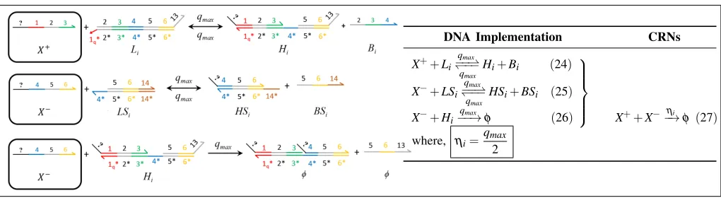
−−→φ (26) X++X−−η→i φ (27)
where, ηi=
qmax
2
Fig. 9: Annihilation reactionX++X−−→ηi φ: The DSD diagram shows degradation of auxiliary speciesX+andX−by means of moleculesLiandLSi. The reaction dynamics are separated into fast and slow time scales such that,X+andX−are sequestered
into intermediate species through reaction with Li andLSi at a fast reaction rate, while X− degrades into waste by reacting
withHi at a slower rate. The initial concentrations ofX+andX−must be scaled by a factor of 2 (let,ξ = 2, hence,X0+ = 1ξ nM andX0−= 0.5ξ nM) to attenuate for the sequestering effect of the fast dynamics; as adapted from [8].
and a proportional gain, implemented as:
X1±−k→p X1±+A±, (28a)
X2±−→kc X2±+A±, (28b)
A±−k→d φ, (28c)
A++A−−→η φ. (28d)
Here, the signal X1 is the input and A is the output.
Furthermore,kpandkcdenote the catalytic reaction rates while kd denotes the degradation rate. The values of these rates are
given in Table III. Using mass action kinetics, the following ODE representation is obtained for the PI controller:
dX2
dt = kIX1, (29)
dA
dt = kpX1+kcX2−kdA. (30)
E. DNA implementations
The linear components of the feedback control system, i.e. the subtractor and PI controller [8], are built using a combination of catalysis–Fig. 7, degradation–Fig. 8 and annihilation–Fig. 9 reactions. The nonlinear components, i.e. the QSM controller and the process to be controlled are constructed based on catalysis–Fig. 5 and bimolecular–Fig. 6 reactions.
Note that the catalysis reactions (9) and (18) in Figs. 5 and 7, respectively, produce different output species depending on the domain composition of the reactant auxiliary species. Species G±i and Ti±, which are partially double stranded DNAs, and single strands of O±i , can be observed to have different domain compositions in Fig. 5 and Fig. 7. As a result, in (9) two different products,X2±andX3±, are obtained whereas, in (18) the single species X±is reproduced.
The domain 1∗q in Figs. 5–9 denotes the subsequence of domain 1 that may be the same length as 1 but contains
some mismatched bases over the displacement domain. The reaction rate of 1∗q is however tuned to rateqi [11] and other
corresponding reaction rates are set by following the notation from [8] and [11]. Initial concentrations of the auxiliary species G±i
0, T
±
i0, L
±
i0, B
±
i0, LS
±
i0, BS
±
i0 are set toCmax=1000 nM. In Fig. 6, which gives the DNA implementation of the bimolecular CRN, the concentrations of Ti±, L±i , B±i remain constant throughout the process [11]. All the other initial concentrations for the remaining species are set to zero.
The rest of this manuscript investigates the closed loop performance properties of the QSM controller, when compared with a linear time-invariant controller synthesized according to the methodologies proposed in [8] and [10]. We re-emphasize that the distinguishing feature of our nonlinear controller (and process to be controlled) is the use of bimolecular reactions; the linear time-invariant systems synthesized in [8] and [10] use unimolecular reactions only.
IV. SIMULATION RESULTS
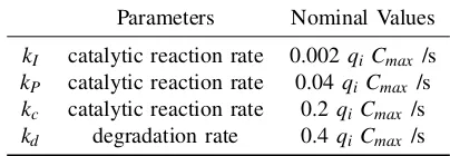
In the following simulations, all reaction rates and total substrate values have been set to the nominal values given in Table I to III. The second order reaction rates are tuned within the practical experimental limits (a maximum value of 107 /M/s) and catalysis, degradation, annihilation rates have been chosen in terms of DNA implementation reaction rates,
qi and initial concentration of auxiliary species,Cmax.
Parameters Nominal Values
Sqsm total substrate 4 nM X3 tuning parameter 0.1 nM
kb1 forward binding rate 10
7 /M/s
kb2 forward binding rate 10
7 /M/s
kc1 catalytic reaction rate 100 qi Cmax /s
[image:8.612.52.562.49.189.2]kc2 catalytic reaction rate 50 qiCmax /s
0 25,000 50,000 75,000 100,000 −4
−2 0 2 4
B
0 1000 2000 3000 4000
2 4
Time (sec)
Concentration (nM)
A
Reference Input (U)X3 = 0.1 nM X
3 = 0.5 nM
Fig. 10: Closed loop tracking response obtained using the QSM controller. Here, the reference inputU is a square wave of magnitude 4 nM. The transient response can be made faster by reducing the controller tuning parameterX3. The subfigure
”B” is a zoomed-in version of the subfigure ”A” to better illustrate the transient response in the region of interest.
Initial values of the signals A, B, X2, X4 are set to zero,
i.e. A0=B0 =X20 =X40 =0 nM. For the PI controller, the nominal values of reaction rates and kinetic constants are shown in Table III and the initial concentrations of the non-auxiliary species in equations (23)-(28) are set to zero, i.e. X20 =A0=0 nM. For the subtractor, ks is set to its nominal value of 3000·qi·Cmax/s where DNA implementation
reaction ratesqi=800 /M/s (i=1,2, ...,21),qmax=107 /M/s
and initial concentration of auxiliary species,Cmax=1000 nM.
The reaction rate of annihilation, η, is set to 10·qiCmax /s.
0 2000 4000 6000 8000 10,000
3.5 4 4.5
Time (sec)
Output (Y)
[image:9.612.53.296.61.253.2]Reference Input (U) Sliding Mode Controller QSM Controller
Fig. 11: Closed loop responses with quasi and ideal sliding mode controllers: the undesirable phenomenon of chattering, i.e., high frequency oscillations, is observed in the closed loop response if the ideal SMC controller is used, but is avoided by the QSM controller.
0 25,000 50,000 75,000 100,000
−6 −4 −2 0 2 4
Time (sec)
Concentration (nM)
Reference Input (U) k
P = 0.04*qi*Cmax
[image:9.612.315.559.64.260.2]kP = 0.14*qi*Cmax
Fig. 12: Closed loop tracking response obtained using a PI controller. The transient response can be made faster by in-creasing the value of the controller tuning parameterkPalbeit
at the cost of introducing progressively larger overshoots.
A square-wave input was chosen for the reference signal
U to be tracked by the process output, in line with standard practice in control theory, since such signals generally result in the most challenging possible tracking problem for the control system (the output must track signals that are changing infinitely fast, in both directions). The magnitude of the square wave was chosen to be sufficiently large that it excites the nonlinear dynamics of the process to be controlled. Fig. 10 shows the closed loop tracking response for the system shown in Fig. 1 when the QSM controller is used. The outputY tracks the inputU with a settling time of 2500s if X3 is set to 0.1
nM . As shown in Fig. 11, the QSM controller also avoids the problem of chattering that is encountered when its limiting case, i.e., the ideal SMC, is used. Fig. 12 shows the closed loop tracking response for the system shown in Fig. 1 when
Parameters Nominal Values
kr1 forward binding rate 500×10
3 /M/s
kr2 catalytic reaction rate 2×10
3 q
iCmax /s kr3 degradation rate 10×10
−3 q
[image:9.612.57.277.520.670.2]iCmax /s XTotal total amount ofX5+X6 3 nM
TABLE II: Process to be controlled — parameter values
Parameters Nominal Values
kI catalytic reaction rate 0.002qiCmax /s kP catalytic reaction rate 0.04qi Cmax /s kc catalytic reaction rate 0.2qiCmax /s kd degradation rate 0.4qiCmax /s
[image:9.612.335.537.648.718.2]0 25,000 50,000 75,000 100,000 −4
−2 0 2 4
A
Concentration (nM)
0 1000 2000 3000 4000
2 4
Time (sec)
B
Reference Input (U) X
3 = 0.1 nM
[image:10.612.52.300.58.253.2]X3 = 0.5 nM
Fig. 13: Closed loop tracking response obtained by using the QSM controller after accounting for retroactivity effects.
the PI controller is used. The closed loop response dynamics that can be achieved with the PI controller are approximately an order of magnitude slower than those achieved using the QSM controller.
The closed loop responses shown in Figs. 10 and 12 assume perfect modularity of the different elements of the feedback system shown in Fig. 1, i.e. interconnection of elements does not change their dynamic response. Although this assumption is routinely made in the vast majority of systems traditionally encountered in engineering disciplines, it has recently been es-tablished that it does not hold for many biomolecular feedback systems, [19], since it often happens that different modules share the same molecular species. The concept of retroactivity has been introduced to quantify the manner in which the interconnection of two modules changes their dynamics with respect to their behaviour when isolated, [20], [21]. For the system under consideration here, it should be noted that the interconnection of modules containing only unimolecular reactions produces no retroactivity effects. For example, in the context of Fig. 1, the interconnection of the subtractor and the PI controller will feature no retroactivity. However, if the system is an interconnection of two modules, one of which comprises unimolecular reactions while the other features bimolecular reactions (e.g. the subtractor and QSM controller) then it will feature a unidirectional retroactivity, since the ODE representation of the subtractor must consider the chemical reactions describing the downstream QSM controller. For the QSM, retroactivity affects the ODEs of two state variables as follows:
dX1
dt = ks(U−Y−X1) −kb1X1B+kc1X2
| {z }
retroactivity
, (31)
dA
dt = kc1X2−kb2AX3 −kr1AX5
| {z }
retroactivity
. (32)
The additional term (−kb1X1B+kc1X2) in equation (31)
0 25,000 50,000 75,000 100,000
−4 −2 0 2 4
Time (sec)
Concentration (nM)
Reference Input (U) k
P = 0.04*qi*Cmax
k
P = 0.14*qi*Cmax
Fig. 14: Closed loop tracking response obtained using the PI controller after accounting for retroactivity effects.
quantifies the retroactivity imposed by the downstream QSM controller on the upstream subtractor through the shared signalX1, while the additional term (kr1AX5) in equation (32) quantifies the retroactivity effects between the QSM controller and the process to be controlled through the shared signalA. As shown in Fig. 13, the nonlinear QSM controller is highly robust to retroactivity effects, with the major change to the closed loop response being a small reduction in overshoot. In the case of the PI controller, retroactivity affects the ODE of only one state variable, due to the interconnection of the controller and process to be controlled, as follows:
dA
dt = kpX1+kcX2−kdA −kr1AX5
| {z }
retroactivity
. (33)
As shown in Fig. 14, for the PI controller the presence of retroactivity results in significant changes in the closed loop response, which is now extremely sluggish - for akpvalue of
0.04 qi Cmax the controller is not able to track the reference
signal even after 50,000 seconds. Understanding the precise structural reasons for the strong robustness to retroactivity effects displayed by the QSM controller is the subject of current research by the authors.
V. CONCLUSIONS AND FUTURE WORK
[image:10.612.312.558.61.259.2]chemical reactions into enzyme-free, entropy/enthalpy driven DNA reactions. Simulation results indicate that, compared to a traditional PI controller, the implemented quasi sliding mode controller results are dramatically faster and more accurate in tracking of reference signals, even in the presence of retroactivity. The proposed design approach is highly modular, fully exploits the inherently nonlinear nature of biomolecular reaction kinetics, and makes for the first time a direct link between the biological concept of ultrasensitivity and the engineering theory of sliding mode control.
Several avenues for further research are opened up by this study. For successful implementation of complex feedback control circuits it will be essential to understand the trade-offs between system performance and complexity (particularly in terms of the number of chemical reactions to be imple-mented experimentally), as well as the effect of experimental uncertainties on closed loop performance (e.g. robustness to variations in reaction rates, etc). It would thus be interesting to investigate whether there are alternative sets of CRNs that could implement a QSM controller using fewer chemical reactions. Sliding mode controllers are only one of many potential nonlinear control schemes that could potentially be implemented using DNA-based chemistry, and much work remains to be done to forge closer links between nonlin-ear control theory, chemical reaction network theory, and the experimental realities of nucleic acid implementations of complex dynamical systems. The treatment in this paper has focussed on deterministic CRNs, but there has been much recent work on CRNs within a stochastic systems framework that could also be applied in the context of the design of biomolecular controllers. Lastly, while the assumption of well-mixed conditions in in vitro systems seems valid, the imple-mentation of DNA-based circuits in vivo will require careful consideration of spatial factors, motivating the extension of the underlying design framework to include partial differential equation-based models.
VI. ACKNOWLEDGMENTS
We gratefully acknowledge financial support from EPSRC and BBSRC via research grant BB/M017982/1 and from the School of Engineering of the University of Warwick.
REFERENCES
[1] J. Stapleton, K. Endo, Y. Fujita, K. Hayashi, M. Takinoue, H. Saito, and T. Inoue, “Feedback Control of Protein Expression in Mammalian Cells
by Tunable Synthetic Translational Inhibition”,ACS Synthetic Biology,
vol. 1, no. 3, pp. 83–88, 2012.
[2] O. Andries, T. Kitada, K. Bodner, N. Sanders, and R. Weiss, “Synthetic Biology Devices and Circuits for RNA–based ‘Smart Vaccines’: A
Propositional Review”,Expert Review of Vaccines, vol. 14, no. 2 , pp.
313–331, 2015.
[3] B. Andrews and P. Iglesias, “Control Engineering and Systems Biology” inMathematical Methods for Robust and Nonlinear Control, pp. 267–288. Springer London, 2007.
[4] M. Feinberg, Lectures on Chemical Reaction Networks, Notes of
Lec-tures Given at the Mathematics Research Center of the University of Wisconsin, [Online]. Available: http://www.che.eng.ohio-state.edu/ FEIN-BERG/LecturesOnReactionNetworks, 1979.
[5] M. Bilotta, C. Cosentino, D. G. Bates and F. Amato, “Retroactivity Analysis of a Chemical Reaction Network Module for the Subtraction
of Molecular Fluxes”,in Proceedings of the 37th IEEE Engineering in
Medicine and Biology Conference, Milano, 2015.
[6] C. Briat, A. Gupta and M. Khammash, “Antithetic Integral Feedback Ensures Robust Perfect Adaptation in Noisy Biomolecular Networks”, Cell Systems, vol. 2, no. 1, pp. 15–26, 2016.
[7] C. Briat, A. Gupta and M. Khammash, “Antithetic integral feedback: A New Motif for Robust Perfect Adaptation in Noisy Biomolecular Networks”, bioRxiv, doi: http://dx.doi.org/10.1101/024919, 2015. [8] K. Oishi and E. Klavins, “Biomolecular Implementation of Linear I/O
Systems”,IET Systems Biology, vol. 5, no. 4, pp. 252–260, 2011.
[9] M. Pedersen and B. Yordanov, “Programming Languages for Circuit
Design”,Computational Methods in Synthetic Biology, pp. 81–104, 2014.
[10] B. Yordanov, J. Kim, R. Petersen, A. Shudy, V. Kulkarni and A. Phillips,
“Computational Design of Nucleic Acid Feedback Control Circuits”,ACS
Synthetic Biology, vol. 3, no. 8, pp. 600–616, 2014.
[11] D. Soloveichik, G. Seelig and E. Winfree, “DNA as a Universal Substrate
for Chemical Kinetics”,Proceedings of the National Academy of Sciences,
USA, vol. 107, no. 12, pp. 5393–5398, 2010.
[12] Y. -J. Chen, N. Dalchau, N. Srinivas, A. Phillips, L. Cardelli, D. Solove-ichik and G. Seelig, “Programmable Chemical Controllers made from
DNA”,Nature Nanotechnology, vol. 8, pp. 755762, 2013.
[13] N. Srinivas, T. Ouldridge, P. ˘Sulc, J. Schaeffer, B. Yurke, A. Louis,
J. Doye and E. Winfree, “On the Biophysics and Kinetics of
Toehold-mediated DNA Strand Displacement”,Nucleic Acids Research, vol. 41,
pp. 10641–10658, 2013.
[14] Y. Shtessel, C. Edwards, L. Fridman, A. Levant, “Introduction: Intuitive
Theory of Sliding Mode Control” inSliding Mode Control and
Observa-tion, pp. 1–42. Springer New York, 2014.
[15] C. Edwards and S. Spurgeon, “Sliding Mode Control” inSliding Mode
Control: Theory and Applications, CRC Press, 1998.
[16] V. Utkin, “Scope of the Theory of Sliding Modes” inSliding Modes in
Control and Optimization, pp. 1–11. Springer Berlin Heidelberg, 1992.
[17] H. Khalil, “Nonlinear Design Tools” inNonlinear Systems, pp. 551–625.
New Jersey Prentice Hall, 2002.
[18] B. Rauzan, E. McMichael, R. Cave, L. Sevcik, K. Ostrosky, E. Whitman, R. Stegemann, A. Sinclair, M. Serra, A. Deckert, “Kinetics and
Thermo-dynamics of DNA, RNA, and Hybrid Duplex Formation”,Biochemistry,
vol. 52, no. 5, pp. 765–772, 2013.
[19] D. Del Vecchio, A. Ninfa and E. Sontag, “Modular Cell Biology:
Retroactivity and Insulation”,Molecular Systems Biology, vol. 4, no. 1,
2008.
[20] D. Del Vecchio and S. Jayanthi, “Retroactivity Attenuation in Tran-scriptional Networks: Design and Analysis of an Insulation Device”, Proceedings of IEEE Conference on Decision and Control, pp. 774–780, Cancun, Mexico, 2008.
[21] S. Jayanthi, K. S. Nilgiriwala and D. Del Vecchio, “Retroactivity
Controls the Temporal Dynamics of Gene Transcription”ACS synthetic
biology, vol. 2, no. 8, pp. 431–441, 2013.
[22] R. Sawlekar, F. Montefusco, V. Kulkarni, and D. G. Bates, “Biomolec-ular Implementation of a Quasi Sliding Mode Feedback Controller
based on DNA Strand Displacement Reactions”, Proceedings of IEEE
Engineering in Medicine and Biology Conference, pp. 949–952. Milan, Italy, 2015.
[23] D. Zhang, “Towards Domain-Based Sequence Design for DNA Strand
Displacement Reactions”, inDNA Computing and Molecular
Program-ming, pp. 162–175. Springer Berlin Heidelberg, 2011.
[24] C. Thachuk, “Logically and Physically Reversible Natural Computing:
A Tutorial” in Reversible Computation, pp. 247–262. Springer Berlin
Heidelberg, 2013.
[25] M. R. Lakin, S. Youssef, F. Polo, S. Emmott and A. Phillips, “Visual DSD: A Design and Analysis Tool for DNA Strand Displacement
Systems”,Bioinformatics, vol. 27, no. 22, pp. 3211–3213, 2011.
[26] D. Zhang and E. Winfree, “Control of DNA Strand Displacement
Kinetics using Toehold Exchange”,Journal of the American Chemical
Society, vol. 131, no. 47, pp. 17303–17314, 2009.
[27] J. Watson and F. Crick, “Molecular Structure of Nucleic Acids”,Nature,
vol. 171, no. 4356, pp. 737–738, 1953.
[28] R. Machinek, T. Ouldridge, N. Haley, J. Bath and A. Turberfield, “Programmable Energy Landscapes for Kinetic Control of DNA Strand
Displacement”,Nature Communications, vol. 5, 2014.
[29] A. Goldbeter and D. Koshland, Jr, “An Amplified Sensitivity arising
from Covalent modification in Biological Systems”,Proceedings of the
National Academy of Sciences, USA, vol. 78, no. 11, pp. 6840–6844, 1981.
[30] Q. Zhang, S. Bhattacharya and M. Andersen, “Ultrasensitive Response
Motifs: Basic Amplifiers in Molecular Signalling Networks”,Open
[31] C. Y. Huang, and J. E. Ferrell, Jr., “Ultrasensitivity in the
Mitogen-Activated Protein Kinase Cascade”,Proceedings of the National Academy
of Sciences, USA, vol. 93, no. 19, pp. 10078–10083, 1996.
[32] C. Gomez-Uribe, G. C. Verghese and L. A. Mirny, “Operating Regimes
of Signaling Cycles: Statics, Dynamics, and Noise Filtering”, PLoS
Computational Biology, vol. 3, no. 12, pp. e246, 2007.
[33] K. J. Astrom and T. Hagglund, “PID Control-Theory, Design and
Tuning” inAdvanced PID Control, ISA - The Instrumentation, Systems,
and Automation Society, Research Triangle ParN, NC, 2005.
[34] G. Franklin, J. D. Powell and A. Emami-Naeini, “A First Analysis of
Feedback” inFeedback Control of Dynamic Systems, Prentice–Hall, 2009.
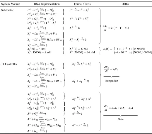
VII. APPENDIX
System Module DNA Implementation Formal CRNs ODEs
(a) QSM Controller X1±+L±1 −−)q−−1*
qmax
H1±+B±1
B±+H1±−−→qmax O±1 +φ X1±+B±
kb1 −−→X2± O±1+T1±−−→qmax X2±
X2±+G±2 −q→2 φ+O±2 X2±
kc1
−−→A±+X1± O±2+T2±−−→qmax A±+X1±
X2++L3 qmax
−−* )−− qmax
H3+B3
X2−+LS3 qmax
−−* )−− qmax
HS3+BS3 X2++X
− 2
η
−→φ
X2−+H3 qmax
−−→φ dA
dt =kc1X2−kb2AX3
A++L4 qmax
−−* )−− qmax
H4+B4
A−+LS4 qmax
−−* )−− qmax
HS4+BS4 A++A−
η
−→φ
A−+H4 qmax
−−→φ dX2
dt =kb1X1B−kc1X2
A±+L±5 −−)q−−5* qmax
H5±+B±5
X3±+H5±−−→qmax O±5+φ A±+X3±−k−b2→X4±
O±5+T5±−−→qmax X4± dX4
dt =kb2AX3−kc2X4
X4±+G±6 −→q6 φ+O±6 X4±−k−c2→B±+X3± O±6+T6±−−→qmax B±+X3±
X4++LS7 qmax
−−* )−− qmax
H7+B7
dB
dt =−kb1X1B+kc2X4
X4−+LS7 qmax
−−* )−− qmax
HS7+BS7 X4++X
− 4
η
−→φ
X4−+H7 qmax
−−→φ
B++L8 qmax
−−* )−− qmax
H8+B8
B−+LS8 qmax
−−* )−− qmax
HS8+BS8 B++B−
η
−→φ
B−+H8 qmax
−−→φ
(b) Process A±+L±9 −−)q−−9*
qmax
H9±+B±9
to be controlled X5±+H9±−−→qmax O±9+φ A±+X5±
kr1 −→X6±
O±9+T9±−−→qmax X6± dX5
dt =−kr1AX5+kr2X6
X6±+G±10−q−10→φ+O±10
X6±−→kr2 Y±+X5±
O±10+T10±−−→qmax Y±+X5± dX6
dt =kr1AX5−kr2X6
Y±+G±11−q−11→φ Y±
kr3
−→φ
Y++L12 qmax
−−* )−− qmax
H12+B12
dY
dt =kr2X6−kr3Y
Y−+LS12 qmax
−−* )−− qmax
HS12+BS12 Y++Y−
η
−→φ
Y−+H12 qmax
[image:13.612.73.534.63.685.2]−−→φ
System Module DNA Implementation Formal CRNs ODEs
(c) Subtractor U±+G±13−q−13→φ+O13± U±−→ks U±+X1±
O±13+T13±−−→qmax U±+X1±
Y±+G±14−q−14→φ+O±14 Y±−→ks Y±+X1∓ O±14+T14±−−→qmax Y±+X1∓
X1±+G±15−q−→15 φ X1±−→ks φ dX1
dt =ks(U−Y−X1) X1++L16
qmax
−−* )−− qmax
H16+B16
X1−+LS16 qmax
−−* )−− qmax
HS16+BS16 X1++X
− 1
η
−→φ
X1−+H16 qmax
−−→φ
X1+(0) =4 nM
X1+(0) =8 nM
X1(t) = 4×10⁻⁹ t∈[0,50000)
X1−(50000) =8 nM X1−(50000) =16 nM −4×10⁻⁹ t∈[50000,100000)
(d) PI Controller X1±+G±17−−→q17 φ+O±17 X1±−k→I X1±+X2±
O±17+T17±−−→qmax X1±+X2± dX2
dt =kIX1 X2++L18
qmax
−−* )−− qmax
H18+B18
| {z }
X2−+LS18 qmax
−−* )−− qmax
HS18+BS18 X2++X
− 2
η
−→φ Integration
X2−+H18 qmax
−−→φ
X1±+G±19−q−19→φ+O±19
O±19+T19±−−→qmax X1±+A± X1±−→kP X1±+A± X2±+G±20−q−20→φ+O±20
O±20+T20±−−→qmax X2±+A± X2±−k→c X2±+A± dA
dt =kpX1+kcX2−kdA
A±+G±21−q−21→φ A±−k→d φ
| {z }
A++L22 qmax
−−* )−− qmax
H22+B22
Gain
A−+LS22 qmax
−−* )−− qmax
HS22+BS22 A++A−
η
−→φ
A−+H22 qmax
−−→φ
[image:14.612.65.584.146.603.2]