Active Filter Control Method Based on Direct Power
Control for Compensating Reactive Powers due to
Unbalanced Voltages and Nonlinear Loads
E. Abirii *, M.R. Salehiii and A. Abrishamifariii
i* Corresponding Author, E. Abiri is with the Department of Electrical Engineering, Shiraz University of Technology (SUTECH), Shiraz, Iran (e-mil: [email protected])
ii M. R. Salehi is with the Department of Electrical Engineering, Shiraz University of Technology (SUTECH), Shiraz, Iran (e-mil: [email protected])
iii A. Abrishamifar is with the Department of Electrical Engineering, Iran University of Science and Technology (IUST), Tehran, Iran, (email: [email protected])
ABSTRACT
Active filters have proven to be more effective than passive techniques to improve power quality and to solve harmonic and power factor problems due to nonlinear loads. This paper proposes a control scheme based on the instantaneous active and reactive power. The inverter of this active filter is a three-phase, two-level converter. Space vector technique is used as modulators and pattern generators for the Pulse Width Modulated converter. Virtual Flux and a Phase Locked Loop based on a Double Synchronous Reference Frame cause this control system be resistant to the majority of line voltage disturbances. Good dynamic response, independent control of active and reactive powers and also unity power factor of converter are advantages of the proposed method. The operation of the proposed control strategy is verified in MATLAB simulation environment.
KEYWORDS
active filter, DPC, power quality, harmonics .
1. INTRODUCTION
Power quality issues are rising in importance, particularly for highly integrated plants that are sensitive to distortions or voltage dips. In most countries, there exist regulations which place limits on the distortion and unbalance that a customer can inject to a distribution system. These regulations may require the installation of filters on customer premises.
Conventional active filters are implemented using two cascaded loops, a current control loop and a dc capacitor voltage regulation loop. A three-phase, two-level converter is usually used to implement active filter. Conventional carrier or space vector techniques are also used as modulators and pattern generators for the Pulse Width Modulated (PWM) converter [1],[2].
Active filter, based on PWM voltage sources converters, is becoming a viable solution to improve power quality in distribution systems. A number of new techniques have recently been proposed to control PWM converters [3]-[5].
One method called direct power control (DPC), is based on instantaneous direct active and reactive power control [2],[3]. This method can be used for active filter control [6],[7]. In DPC, there are no internal current control loops and no PWM modulator block, because the converter switching states are appropriately selected by a switching table related to the instantaneous errors between the commanded and estimated values of active and reactive power. This method uses the estimated Virtual Flux (VF) vector instead of the line voltage vector in the control loop [7].
Amirkabir / Electrical & Electronics Engineering / Vol . 41 / No.2 / Fall 2009
2
VF and DSRF-PLL cause this control system be resistant to majority of line voltage disturbances. This assures proper operation of the system for abnormal and failure grid conditions.
The operation of proposed control strategy is verified in SIMULINK/MATLAB simulation environment.
2. CONTROL SHEME OF ACTIVE FILTER
Figure 1 shows three phase voltage source converter (SVM) that is connected to a grid. The converter active and reactive powers are[8]:
) 1 ( = + + + + +
a b c
a b c
dc a a b b c c
d i d i d i
p L( i i i )
dt dt dt
U ( S i S i S i )
) 2 ( )]} i i ( S ) i i ( S ) i i ( S [ U ) i dt di i dt di ( L { q b a c a c b c b a dc a c c a − + − + − − − = 3 3 1
In these equations, Sa, Sb and Sc are switching states,
dc
U is the converter DC voltage,
i
a ,i
b andi
c are ACsupply phase current and
L
is supply phase inductor. The first term in (1) and (2) is the inductor power and the second term is the converter power.C abc
[ i ] L
dc C Udc a
S Sb Sc
a
S Sb Sc
C abc [U ] abc S] U [
Figure 1: A converter connected to a grid.
From an economical point of view, simplicity, greater reliability and separation of power stage and control, AC line voltage sensors are replaced by flux estimator.
) 3 (
∫
= u dt
Ψ
If uab, ubc and uca are the AC line to line voltages and
Ca
i
andi
Cb are the converter currents, then uS and iCcan be written[2]:
) 4 ( ⎥ ⎦ ⎤ ⎢ ⎣ ⎡ ⎥ ⎦ ⎤ ⎢ ⎣ ⎡ = ⎥ ⎦ ⎤ ⎢ ⎣ ⎡ = bc ab S S S u u u u u 2 3 0 2 1 1 3 2 β α ) 5 ( ⎥ ⎦ ⎤ ⎢ ⎣ ⎡ ⎥ ⎦ ⎤ ⎢ ⎣ ⎡ = ⎥ ⎦ ⎤ ⎢ ⎣ ⎡ = Cb Ca C C C i i i i i 3 2 3 0 2 3 3 2 β α
In these equations, uSα and uSβ are the line voltage
and
i
Cα andi
Cβ are the converter current in α −β coordinates.According to the current direction, the line voltage uS
can be expressed as the sum of the inductor voltage (uI) and the converter voltage (uC).
) 6 (
S C I
u =u +u
Also, the converter voltage equations in α −β
coordinates are[2]: ) 7 ( )) S S ( S ( Udc
uC = a − b+ c
2 1 3 2 α ) 8 ( ) S S ( Udc
uC = b− c
2 1 β
The utility voltages can be written [1]:
) 9 ( C S C d i
u u L
dt
= +
By considering (3) and (9), the estimated virtual flux will be: ) 10 (
{
}
( )= = +∫
∫
S S est C Creal u dt
u dt Li
α α α ψ ) 11 (
{
−}
= = +∫
∫
S ( est )
S
C C
imaginary u dt
u dt Li
β
β β
ψ
Also instantaneous active and reactive powers are: ) 12 ( } i . u Im{ q , } i . u Re{ p C * S C * S = =
where * denotes the conjugate line current vector. According (3), the line voltage uS can be expressed by line flux
S ψ as[1]: (13)
(
)
S t j S t j S t j S t j S S S j e dt d e j e dt d e dt d dt d u Ψ ω Ψ Ψ ω Ψ Ψ Ψ ω ω ω ω + = + = = =where Ψ S denotes the space vector and
ψ
S its amplitude.Current, VF and voltage vectors in α −β coordinates have shown in Fig.2. For power estimation in α −β
coordinates, S
ψ must be expressed by ΨSα andΨSβ.
) 14 (
(
)
Ψ Ψ = ++ Ψ + Ψ
S S S S S d d u j dt dt j j α β α β ω ) 15 (
(
)
(
)
* * S S CS S S
C C
d d
u i j j j
dt dt
i ji
α β α β
α β
ω
Ψ Ψ
⎧ ⎫
=⎨ + + Ψ + Ψ ⎬
⎩ ⎭
) 16 ( )
i i
(
i dt d i dt d p
C S C S
C S C
S
α β β α
β β α
α
ψ ψ
ω
ψ ψ
−
+ ⎥⎦ ⎤ ⎢⎣ ⎡ + ⎥⎦ ⎤ ⎢⎣ ⎡ =
) 17 ( )
i i
(
i dt d i dt d q
C S C S
C S C
S
β β α α
α β β
α
ψ ψ
ω
ψ ψ
+
+ ⎥⎦ ⎤ ⎢⎣ ⎡ + ⎥⎦ ⎤ ⎢⎣ ⎡ − =
For sinusoidal and balanced line voltage the derivatives of the flux amplitudes (
β
ψ
⎡ ⎤
⎢ ⎥
⎣ ⎦
s d
dt
and
α ψ
⎡ ⎤
⎢ ⎥
⎣ ⎦
s d
dt
)
are zero. The instantaneous active and reactive powers can be computed as [1]:
) 18 (
) i i
(
p=ω ψSα Cβ −ψSβ Cα
) 19 ( )
i i
(
q=
ω
ψ
Sα Cα +ψ
Sβ CβFigure 2: Current, VF and voltage vectors in α −β coordinates.
3. ACTIVE FILTER CONTROL BLOCK
Active filter control block supplying a three phase nonlinear load is shown in Fig.3.
According to (5), by the measured DC link voltage dc
U , the converter current
i
Ca andi
Cband the switching states Sa, Sb and Sc, at first the converter current iscomputed, then, considering (7), (8), (10) and (11), the virtual flux is estimated in VF block.
The active and reactive powers are estimated by (18) and (19). These equations are applied in the power estimation block. The output of this block are pC and
C
q .
In an unbalanced three phase power system, or in a distorted three phase system caused by nonlinear loads, both real and imaginary power are no longer constant, and are expressed by the following:
) 20 (
q ~ q q p ~ p
p= + = +
Where p and q are the average powers and p~ , q~
are the power ripple caused by negative sequence components and harmonics. pL and qL powers are estimated by load currents (iLα and iLβ) and VF (ΨSαand
β
ΨS ). The calculated active and reactive powers are delivered to the high pass filter (HPF) to obtain the alternative value.
As shown in Fig.3, the commanded reactive power Cref
q ( set to zero for unity-power-factor operation ) and
reference active power pCrefvalues (obtained by the
outer proportional–integral (PI) dc voltage controller) are compared to the inverter estimated powers.
4
A. DSRF-PLL
If the voltage line is of distortion, harmonic and unbalance, the sector number is selected erroneously. To detect the virtual flux angle in SVM correctly it is used of PLL named DSRF-PLL[9]. Further improvements regarding DPC operation can be achieved by using careful sector detection with a PLL (Phase-Locked Loop) generator instead of a zero crossing voltage detector to guarantee a very stable and also disturbance free sector detection, even under operation with distorted and unbalanced line voltages. In this case, a DSRF-PLL based on VF is employed.
When the utility voltage is unbalanced, the virtual flux can be written as the following: the VF estimated can be expressed on the α β− stationary reference frame as:
) 21 ( + − + − ⎡ ⎤ = + = ⎢ ⎥ ⎣ ⎦ ⎡ ⎤ + ⎢ ⎥ − ⎣ ⎦ ( ) cos( ) sin( ) cos( ) sin( ) ψ αβ ψ ψ ψ γ
ψ ψ ψ ψ γ
γ ψ γ ) 22 ( ) ( tg α β
ψ ψψ
γ = −1
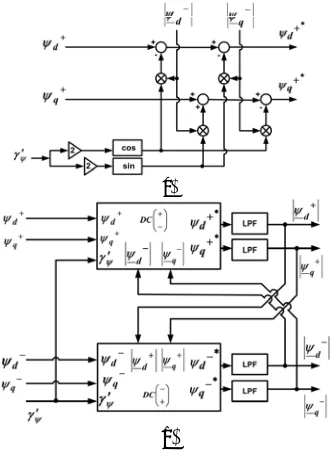
This VF vector is expressed on the double reference frame as shown in Fig.4. In this figure, γψ′ is dq+ angle
in the positive direction and −γψ′ is dq− angle in the
negative direction. In this double reference frame, the d+
and the d− axes are synchronized with ψ+ and ψ−, respectively. Also, dq+ rotates in the positive direction and its angular position is γψ′, and dq− rotates in the
negative direction and its angular position is −γψ′. The expressions of ψ on these reference frames are:
) 23 ( + + + + ⎡ ⎤ ⎡ ⎤ =⎢ ⎥ ⎣= ⎦ = ⎢ ⎥ ⎣ ⎦ ′ ′ ⎡ ⎤ ⎢− ′ ′ ⎥ ⎣ ⎦ d dq
( dq ) ( )
q
( )
T
cos( ) sin( ) sin( ) cos( )
αβ ψ ψ αβ ψ ψ ψ ψ ψ ψ γ γ ψ γ γ ) 24 (
[ ]
) ( ) ( dq q d ) dq ( ) cos( ) sin( ) sin( ) cos( T αβ ψ ψ ψ ψ αβ ψ γ γ γ γ ψ ψ ψ ψ ⎥ ⎦ ⎤ ⎢ ⎣ ⎡ ′ ′ ′ − ′ = = ⎥ ⎥ ⎦ ⎤ ⎢ ⎢ ⎣ ⎡ = −− − −Figure 4: Representation of the flux vectors and reference axes.
Using a PLL structure and regulating appropriately its control parameters, it is possible to obtain γψ′ ≈γψ. Therefore, in small signal it can be taken: The selection of these PLL control parameters are based on a small signal analysis in which are assumed sin(γψ −γψ′)≈γψ −γψ′ , cos(γψ −γψ′) 1≈ and (−γψ −γψ′)≈ −2γψ. So, the flux
components of (23) and (24) can be approximated by:
) 25 ( ) sin( ) ( ) cos( d ψ ψ ψ ψ γ γ γ ψ γ ψ ψ ψ ′ ′ − − ′ + ≈ − − + + 2 2 ) 26 ( ) sin( ) ( ) cos( d ψ ψ ψ ψ γ γ γ ψ γ ψ ψ ψ ′ ′ − − ′ + ≈ + + − − 2 2 ) 27 ( ) cos( ) ( ) sin( ) ( q ψ ψ ψ ψ ψ ψ γ γ γ ψ γ ψ γ γ ψ ψ ′ ′ − − ′ − ′ − ≈ − − + + 2 2 ) 28 ( ) cos( ) ( ) sin( ) ( q ψ ψ ψ ψ ψ ψ γ γ γ ψ γ ψ γ γ ψ ψ ′ ′ − + ′ + ′ − − ≈ + + − − 2 2
As it is clear in (25) to (28), this equations contain the amplitude of ψ+ and ψ− , respectively, and oscillations with 2ω frequency. To obtain the amplitude of ψ+ and
ψ−
and omitting the oscillations with 2ω frequency, it can be used of LPF. But the LPF dynamic response is low. To meet this defect, a decoupling network (DNi) is suggested. DN will be explained in the next section.
I) Decoupling signals in the DSRF
In (25) and (26), the amplitude of the signal oscillation in the d+−q+ axes pertains to the mean value
of the signal in the d−−q− axes, and the reverse. To cancel the oscillations in the d+−q+ axes signals, the decoupling cell (DCii) shown in Fig. 5(a) is suggested. In order to cancel the oscillations in the d−−q− axes signals, the same configuration of the DC can be employed but swapping (-) and (+) superscripts in the variables. Logically, for an accurate operation of both DC’s it is essential to design some method to determine the value of
d ψ + , q ψ + , d ψ − and q ψ − .
response will also be higher, which can increase unstable behavior of the detection system. This is the reason why the value of k should not be too high in order to be able to reduce oscillations in the response and make the detection system more stable. This restriction in the maximum value of k is even more significant when the utility voltages not only present an imbalance at the fundamental frequency but also high order harmonics. It seems logical to establish k =1/ 2, since the dynamic response is fast enough and oscillations do not appear in the amplitude estimation of ψ+.
(a)
(b)
Figure 5: (a) Decoupling cell for canceling the effect of ψ− on the d+–q+ frame signals; (b) Decoupling network of d+–q+ and d−–q− reference frames.
The block diagram of the DSRF-PLL is shown in Fig.6. The tuning parameter for LPF is k =1/ 2 and for PI controller the proportional and integral coefficients are
2 22
p
k = . and ki =246 7. ,respectively.
Figure 6: Block diagram of the DSRF-PLL.
The active and reactive powers are modified using DSRF-PLL and used for careful sector detection.
) 29 ( )
i i
(
pC ωψSα Cβ ψSβ Cα +′ +′
− =
) 30 ( )
i i
(
qC ωψSα Cα ψSβ Cβ +′ +′
+ =
B. Switching Table
Two hysteresis comparators have been used to control both active and reactive powers. dpand dq are the
quantized output of these controllers which have zero or one magnitude. Virtual-flux angle (γψ′ ), dpand dqare the
inputs and Sa, Sb and Sc are the outputs of switching table. γψ′ has low sensitivity to voltage distortion. To reach more accuracy and DPC correct behavior, the number of sectors or hysteresis levels must be increased. As can be seen from Fig.7 the number of sectors are increased into 12 .
Table 1 shows 12 sectors switching table. This table is the best response of DPC and is valid for converter. It is based on the variation of active and reactive powers in SVM sectors.
Figure 7: Twelve sector.
TABLE1
SWITCHINGTABLEFORCONVERTER
1 1
0 0
dp
1 0
1 0
dq sector
010 001
110 100
1
011 101
110 100
2
011 101
010 110
3
001 100
010 110
4
001 100
011 010
5
101 110
011 010
6
101 110
001 011
7
100 010
001 011
8
100 010
101 001
9
110 011
101 001
10
110 011
100 101
11
010 001
100 101
12
4. SIMULATION RESULTS
6
proposed control system is applied under different line voltage conditions and harmonic sources.
The parameters of active filter system are presented in Table 2.
TABLE 2
SIMULATION PARAMETERS
Parameters Value Converter output DC voltage (KV) 20
Utility line voltage (KV) 10
Utility frequency (HZ) 50
Sampling frequency (kHZ) 50
Average switching frequency
(kHZ) 5
Load
R (Ω) 100
Line inductance (mH) 3
DC link capacitor (uF) 470
A. Nonlinear Load
Under nonlinear load condition, a diode rectifier with capacitor load (470µF) is connected in parallel with active filter and distribution system. Active filter makes sinusoidal current and decreases harmonic in the utility current.
Fig.8 shows input line voltage, input current of the nonlinear load, PCC line voltage and utility current when active filter is connected in parallel with a nonlinear load. As can be seen from Fig.8, the proposed active filter can cause a PCC line voltage and utility current wave forms to be sinusoidal. Therefore the harmonics due to nonlinear load have been eliminated by using active filter.
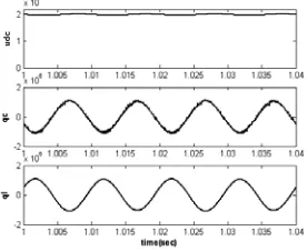
Input DC voltage to the converter and also injected current from converter into the grid are shown in Fig.9.
The compensated reactive power, nonlinear load reactive power and their differences are also shown in Fig.10. As can be seen from this figure, the difference between these powers is little. Therefore the active filter has removed the reactive power generated by nonlinear load.
Fig.11 shows the harmonics of utility current. Total harmonic distortion (THD) is equal to 4.24%. Without active filters THD is 26.8%.
Figure 8: From Up to Down: Nonlinear load voltage and current, PCC voltage and utility current.
Figure 9: From Up to Down: DC voltage of converter and injected current from converter in to the grid.
Figure 10: From Up to Down: Compensated reactive power, nonlinear load reactive power and their differences.
Figure 11: harmonics of utility current.
Fig.12 shows the positive-sequence virtual flux in
α
−β
coordinates (DSRF-PLL outputs) while active filter DSRF-PLL is connected to gridFigure 12: The positive-sequence virtual flux inα −β coordinates (DSRF-PLL outputs).
B. Unbalanced Source
) 31 (
) t sin( u . u
) t sin( u . u
) t sin( u u
m c
m b
m a
3 2 85
0
3 2 25
1
π ω
π ω ω
+ ×
=
− ×
= × =
In the above equations, um is the utility voltage
amplitude.
Fig.13 shows phase voltage and output current of unbalance source, also PCC voltage and the utility current when active filter is connected to grid. As shown in Fig.13 the unbalance system has no impact on utility current and utility sinusoidal current is achieved.
Figure 13: From Up to Down: Unbalanced source voltage and current and utility current.
Fig.14 shows DC voltage and reactive power of the compensator, also reactive power of unbalanced voltage source. This figure shows complete elimination of reactive power produced by unbalanced source in the presence of active filter.
Figure 14: From Up to Down: DC voltage and reactive power of the compensator and reactive power of unbalanced voltage source.
C. Distorted Source
For harmonic source simulation, a voltage source with fifth and seventh harmonic by different amplitude are applied to the each line of distribution system.
sin( ) 0.2*[ sin(5 ) sin(7 )]
2 2
sin( ) 0.2* sin(5 )
3 3
2
0.2* sin(7 )
3
2 2
sin( ) 0.2* sin(5 )
3 3
2
0.2* sin(7 )
3
= + +
= − + + +
−
= + + − +
+
a m m m
b m m
m
c m m
m
u u t u t u t
u u t u t
u t
u u t u t
u t
ω ω ω
π π
ω ω
π ω
π π
ω ω
π ω
(32) The amplitudes of 5th and 7th harmonics are assumed 20% of the fundamental voltage amplitude. Fig.15 shows the distorted source phase voltage, output current of the source, PCC voltage and the utility current while active filter is connected to grid.
As can be seen from Fig.15, the active filter causes a utility current wave form to be sinusoidal.
Fig.16 shows the harmonics of utility current. Total harmonic distortion (THD) is equal to 1.52%. The amplitudes of 5th and 7th harmonics are decreased to 0.2% and 0.8% of the fundamental voltage amplitude, respectively.
Figure 15: From Up to Down: Distorted load voltage and current, PCC voltage and utility current.
Figure16: harmonics of utility current.
5. CONCLUSION
This paper proposes a new method for an active filter. The proposed active filter makes a utility bus voltage sinusoidal at the presence of any unbalance, harmonic or flicker in the source voltage, or unbalance or harmonic in the load current.
VF and DSRF-PLL cause this control system be resistant to the majority of line voltage disturbances.
Good dynamic response, independent control of active and reactive powers and also unity power factor of the utility are advantages of this method.
8
6. REFERENCES
[1] Rahmati A.; Abrishamifar A.; Abiri E.; “Space vector modulation direct power control in an inverter connected to grid and wind turbine”, In Persian, fourteenth electrical conference, Iran, May 2006.
[2] Malinowski M.; “Sensorless control strategies for three-phase PWM rectifiers”, Ph.D. dissertation, Inst. Control Ind. Electron., Warsaw Univ. Technol., Warsaw, Poland, 2001.
[3] Noguchi T.; Tomiki H.; Kondo S.; Takahashi I.; “Direct power control of PWM converter without power-source voltage sensors”, IEEE Trans. Ind. Applicat., vol.34, pp.473-479, May/June 1998. [4] Peng F., Z.; Ott G., W.; Adams D., J.; “Harmonic and reactive
power compensation based on the generalized instantaneous reactive theory for three-phase four-wire systems”, IEEE Trans. Power Elec., vol.13, pp.1174-1181, Nov.1998.
[5] Kwon B., H.; Lim J., H.; “A line-voltage-sensorless synchronous rectifier”, IEEE Trans. Ind. Applicant, vol.14, pp.966-972, sept.1999.
[6] Chen S.; Joos G.; “Direct power control of active filters for voltage flicker mitigation”, Ind. Appl. Conference, Thirty-sixth IAS Annual Meeting, pp.2683-2690, September/October 2001.
[7] Cichowias M.; Malinoaski M.; Kazmierkowski M., P.; Sobczuk D., L.; Rodrigues P.; Pou J.; “Active filtering function of three-phase PWM Boost rectifier under different line voltage conditions”, IEEE Trans. On Ind. Elec., vol.52, no.2, pp.410-419, April 2005. [8] Ohnishi T.; “Three-phase PWM converter/inverter by means of
instantaneous active and reactive power control”, IECON’91, pp.819-824, 1991.
[9] Rodriguez P.; Bergas J.; Pou J.; Candela I.; Burgos R.; Boroyevich D.; “Double synchronous reference frame PLL for power converters control”, IEEE 36th. conf. on power electronic specialists, pp.1415-1421, 2005.
iDecoupling Network