ORIGINAL ARTICLE
Sound Source Localisation for a High-Speed
Train and Its Transfer Path to Interior Noise
Jie Zhang
*, Xinbiao Xiao, Xiaozhen Sheng and Zhihui Li
Abstract
Noise is one of the key issues in the operation of high-speed railways, with sound source localisation and its transfer path as the two major aspects. This study investigates both the exterior and interior sound source distribution of a high-speed train and presents a method for performing the contribution analysis of airborne sound with regard to the interior noise. First, both exterior and interior sound source locations of the high-speed train are identified through in-situ measurements. Second, the sound source contribution for different regions of the train and the relationships between the exterior and interior noises are analysed. Third, a method for conducting the contribution analysis of airborne sound with regard to the interior noise of the high-speed train is described. Lastly, a case study on the side-wall area is carried out, and the contribution of airborne sound to the interior noise of this area is obtained. The results show that, when the high-speed train runs at 310 km/h, dominant exterior sound sources are located in the bogie and pantograph regions, while main interior sound sources are located at the sidewall and roof. The interior noise, the bogie area noise and the sound source at the middle of the coach exhibit very similar rates of increase with increasing train speed. For the selected sidewall area, structure-borne sound dominates in most of the 1/3 octave bands.
Keywords: High-speed train, Interior noise, Sound transfer path, Noise source identification, Exterior noise, Airborne sound
© The Author(s) 2019. This article is distributed under the terms of the Creative Commons Attribution 4.0 International License (http://creat iveco mmons .org/licen ses/by/4.0/), which permits unrestricted use, distribution, and reproduction in any medium, provided you give appropriate credit to the original author(s) and the source, provide a link to the Creative Commons license, and indicate if changes were made.
1 Introduction
In recent years, China’s high-speed railway has developed rapidly. A series of new high-speed lines and high-speed trains have been built. Therefore, new challenges have emerged, necessitating further research. Noise is one of the key issues for operating high-speed railways [1–5], with sound source localisation and its transfer path as the two main aspects.
The major noise sources for a high-speed train are wheel/rail rolling noise and pantograph aerodynamic noise [6, 7]. Remington [8] and Thompson [9] conducted comprehensive research on mechanism of generation and ways to predict the wheel/rail noise. Wu et al. [10] stud-ied the rolling noise generated by wheel/track parametric excitation. They found that the use of the moving irregu-larity model without considering wheel/track parametric excitation may lead to underestimation of the noise level
at high speeds. Sheng et al. [11] extended the Fourier-transform-based method to obtain revised equations that are appropriate for predicting sound radiation from slab high-speed railway tracks. Zhang et al. [12] investigated the effects of ballast on sound radiation from the rail-way track, with the conclusion that ballast vibration can increase the sound radiation by 1–4.5 dB for frequencies between 20 Hz and 300 Hz at the full scale, whereas at higher frequencies the effect is negligible. Nagakura [13] performed wind tunnel tests using a 1/5 scale Shinkansen train model and analysed the distribution of aerodynamic noise sources. Latorre Iglesias et al. [14] proposed a semi-empirical component-based model to predict the aerody-namic noise from train pantographs.
Eliminating noise sources is the most direct and effec-tive method of noise control. Therefore, it is important to study the sources and the associated mechanisms of noise generation. Furthermore, studying sound source localisation and its transfer path is also important, because these two aspects directly influence noise control measures. Mellet et al. [15] investigated the contribution
Open Access
*Correspondence: [email protected]
of the aerodynamic/rolling noise for high-speed trains. They concluded that whether or not the rolling noise is the most important source, it depends on not only the train speed but also the wheel/rail surface conditions. Zea et al. [16] introduced a wavenumber-domain filter-ing technique, referred to as wave signature extraction, to separate the rail contribution to the total pass-by noise. The advantage of the method is that, in principle, no prior knowledge of the structural properties of the track is needed. Ström [17] used the operational transfer path analysis technique to compare transmission of the out-side noise to the interior noise by different paths within a high-speed train bogie. It is found that the three impor-tant paths in the frequency range analysed are the air-borne transfer path, traction rod and yaw dampers. Fan et al. [18] used the sound intensity and partial coherence methods to identify the most significant sources of the interior noise. They found that the major source of the interior noise is the structural-borne sound radiated by floor vibration. Zhang et al. [19] presented a detailed sta-tistical energy analysis and contribution analysis for the interior noise of a high-speed train. They found that for the studied coach the key factors determining the inte-rior noise are the sidewall vibration, bogie area noise, and floor acoustic transmission loss.
In summary, it is obvious that there are many researches on sound sources and noise transfer paths. However, for high-speed trains, there is still a lack of joint analysis of interior sources and exterior sources, espe-cially the quantitative analysis of the transfer contribution from the exterior to the interior, which is precisely the key to control the interior noise. This study investigates both exterior and interior sound source distributions of a high-speed train and presents a method for contribution analysis of airborne sound to the interior noise. In Sec-tion 2, both exterior and interior sound source locations of a high-speed train are identified through in-situ meas-urements. The sound source contributions of different regions and relationships between the exterior and inte-rior noises are analysed. In Section 3, a method for the contribution analysis of airborne sound to the interior noise of the high-speed train is described. In Section 4, a case study for the sidewall area is then carried out, and the contribution of airborne sound to the interior noise of that area is obtained. Finally, the conclusions are pro-vided in Section 5.
2 Exterior and Interior Sound Source Localisations The measured high-speed train consists of eight coaches. The first, the third, the sixth and the last coaches are trailer car, while the other coaches are motor car. The length, the width and the height (from rail head and not include the pantograph) of the train are, respectively,
209 m, 3.36 m and 4.05 m. There is slab track on the via-duct using UIC 60 rail and WJ-8A fastening. The sidewall height is about 0.68 m relative to the bridge deck.
2.1 Distribution of Exterior Sound Sources
Figure 1 shows a test photograph of the measurement of the exterior noise source of a high-speed train running at 310 km/h, conducted using a 78-channel wheel micro-phone array (B&K WA-0890-F). The diameter of the array is 4 m, and the array centre was 7.5 m away from the centreline of the track and 2 m above the rail surface.
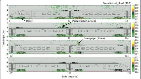
The software B&K NSI array acoustics post-processing was used for the exterior noise source identification anal-ysis. The focus points are all set to be in the plane of the sidewall which is 5.8 m from the microphone array. The method is called rail vehicle moving source beamform-ing (BZ-5939) [20–22]. Figure 2 illustrates the distribu-tion of the exterior noise sources of the train running at 310 km/h.
It can be seen from Figure 2 that the main exterior noise sources of the high-speed train running at 310 km/h are located at the bogie area and pantograph area. The noise generated from the bogie area includes the wheel/rail rolling noise, gear noise, and bogie aerodynamic noise. It can be seen that the sound intensity levels of differ-ent bogies are quite differdiffer-ent. The noise levels decrease from the first to the last bogie. Because the rolling noise and gear noise are approximately equal for each bogie, the main cause of the bogie noise difference is the bogie aerodynamic noise [23, 24]. The aerodynamic noise plays an important role, especially in the first five bogies, when the train is running at a high speed such as 310 km/h.
The side surface of the high-speed train is divided into eight areas, as shown in Figure 3, which are the bogie area, pantograph area, head area, rear area, inter-coach
Figure 1 Measurement photograph of the exterior noise source
Figure 2 Exterior noise source distribution of the high-speed train running at 310 km/h (frequency range: 500–5000 Hz)
area, top area of the coach, middle area of the coach, and bottom area of the coach. The sound power is then obtained by integrating the sound intensity over each area, with each contribution calculated by using
where I(s) is the sound intensity at a discrete point, ∆S is the area of each zone, and S is the total area of all zones.
Figure 4 shows the contributions of different areas to the total sound power. As shown in Figure 4, when the high-speed train runs at 310 km/h, the contributions of the bogie area, bottom area of the coach, and middle area of the coach are relatively high, reaching 33.5%, 21.8%, and 24.1%, respectively. The contributions of the head and inter-coach areas are almost equal, 2.5% and 2.9%, respectively. The rear area shows the lowest contribution, which is only 0.1%. Although the source with one of the highest levels located at pantograph area, as indicated in Figure 2, its contribution is not very large. Because the high sound level only occupies small area, resulting in a low contribution.
The vertical distribution of the sound sources of the high-speed train expresses the intensity of the sound sources in the vertical direction and can be expressed through the single event sound level (SEL), given as
where L is the length of the train, I(l) is the sound inten-sity in the horizontal direction of the carbody, and Iref is the reference sound intensity, equal to 1 pW/m2. The area of the exterior noise source distribution of the high-speed train (as indicated in Figure 3) was 208 m in length
(1) Cs=
�SI(s)ds
SI(s)ds ,
(2)
SEL=10×log10 LI(l)dl
Iref
,
and 6 m in height. The grid step was selected as 0.1 m. Hence, Eq. (2) is the sound intensity integration in the horizontal direction of the beamforming acoustic map.
Figure 5 shows the vertical distribution of the exte-rior noise sources of the high-speed train running at 310 km/h. From Figure 5, when the high-speed train is running at 310 km/h, the maximum sound intensity level in the vertical distribution is 126.3 dBA, corresponding to a height of 0.2 m above the railhead. The minimum sound intensity level of 115.0 dBA corresponds to a height of 1.4 m. Their height difference is 1.2 m, while their sound intensity level difference is 11.3 dBA. For heights from 1.4 m to 5.8 m, the sound intensity level increases with height. During the pass-by time, the sound intensity level in the vertical distribution is maximised in the bogie area, followed by the bottom area of the coach, the pantograph area, the top area of the coach, and the middle area of the coach. This order is somewhat different from the chart of relative contributions of different areas to the total sound power shown in Figure 4. The reason is mainly the way in which we divide the coach area. For example, in Figure 5, the pantograph area covers the entire length of the train; however, in Figure 4, the pantograph area covers only a part of the train area.
2.2 Distribution of Interior Sound Sources
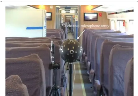
Figure 6 shows the setup used for the measurement of the interior noise sources of the high-speed train running at 310 km/h, performed using a spherical microphone array with 50 channels and 12 cameras (B&K WA1565W004). The diameter of the array is 19.5 cm, which is acoustically much smaller than the dimensions of the coach. The end of the first coach was chosen as a research object, and the
Figure 4 Contributions to the total sound power from different areas
of the train
0 1 2 3 4 5 6
100 105 110 115 120 125 130
SEL (dBA re 1pW/m)
Height (m
)
0.2 m, 126.3 dBA 1.4 m, 115.0 dBA
3.0 m, 119.0 dBA 4.0 m, 119.8 dBA
5.0 m, 121.0 dBA 5.8 m, 122.9 dBA
Figure 5 Vertical distribution of the exterior noise sources of the
array was positioned with its centre at a height of 1.2 m above the interior floor. The interior noise and the exte-rior noise were measured on the same train and at the same time.
The software B&K NSI array acoustics post-process-ing was used for the interior noise source identification analysis, and the method is called spherical harmonics beamforming [25, 26]. Figure 7 illustrates the distribution of the interior noise sources at the end of the first coach.
From Figure 7, the main interior sources at the end of the first coach are located in the sidewall and the roof. However, as indicated in Figure 2, the main exterior noise source of the first coach is the bogie area noise, which is located under the floor. Therefore, the mechanism of the noise transfer from the exterior to the interior of the train needs to be understood. Moreover, even though the exterior and interior sources are located in the same area,
it is important to identify how much noise is transferred through the airborne path and how much through the structure-borne path, because the noise control meas-ures are directly influenced by these factors.
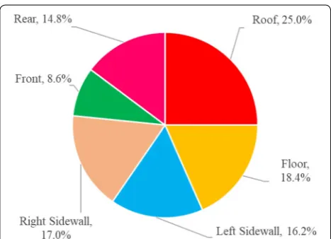
The interior surface at the end of the coach is divided into six areas as shown in Figure 8, which are the roof, left sidewall, right sidewall, floor, front, and rear.
Figure 9 shows the contributions to the total sound power from the different interior areas. It can be seen from Figure 9 that, when the high-speed train runs at 310 km/h, the roof area shows the highest contribution of 25.0%. This is related to the air conditioner noise outside the roof. The contributions of the floor, left sidewall, and right sidewall areas are almost equal and measure 18.4%, 16.2%, and 17.0%, respectively. The front area is associ-ated with the lowest contribution of 8.6%, whereas the contribution of the rear area is 14.8%. More noise comes from the rear than from the front because the measured point is located at the end of the coach.
Therefore, the distribution of sound sources and the contributions to the total sound power from different areas of the exterior and interior are quite different. The interior noise characteristics are not only affected by the exterior sound sources but also related to the sound transfer paths. Before studying the sound transfer path from the exterior to the interior, it is necessary to further analyse the relationship between the exterior and interior noises.
2.3 Relationships between the Exterior Noise and the Interior Noise
Figure 10 shows the dependences of the interior noise, the bogie area noise, and the major exterior sound sources of different areas on the train speed. Because of the lack
Figure 6 Measurement photograph of the interior noise source
identification
of measurement results on the interior noise sources at different speeds, we do not present those data. The inte-rior noise is measured by a microphone positioned 1.2 m above the interior floor at the end of the first coach, and the bogie area noise is measured by a microphone fixed in the middle of the second bogie of the first coach. For both interior noise and bogie area noise, we use sound pressure level, whereas for all the exterior sound sources in different areas, we use sound power level.
As shown in Figure 10, when the train speeds are between 200 km/h and 350 km/h, the interior noise, the bogie area noise, and the major exterior sound sources in different areas all increase with the train speed, with the dependence expressed by the linear regression law as
where a is a coefficient, v is the train speed, L is either the sound pressure level or sound power level, and v0 is the reference speed, which is 200 km/h. Table 1 shows the fitting results, where R2 is the corresponding correlation coefficient. The bigger a is, the faster the noise increases with the train speed.
It can be seen from Table 1 that the interior noise and bogie area noise both increase with the train speed at similar rates. This indicates that the bogie area noise (includes wheel/rail rolling noise and aerodynamic noise) contributes significantly to the interior noise. However, from the measurement results for the exte-rior sound sources, the rates corresponding to the bogie area sound source and bottom of the coach sound source are lower than that of the interior noise. This is related to the details of the noise source measurement, with the results accounting only for the side surface of the coach. However, the bogie area noise directly transfers through the floor from the bottom of the train to the interior. In addition, the increased rates corresponding to the top and middle of the coach are similar to that of the interior noise, which indicates that the outside sources provide important contributions to the interior noise.
3 Sound Transfer Paths from the Exterior to the Interior
3.1 Principle of the Sound Transfer Paths
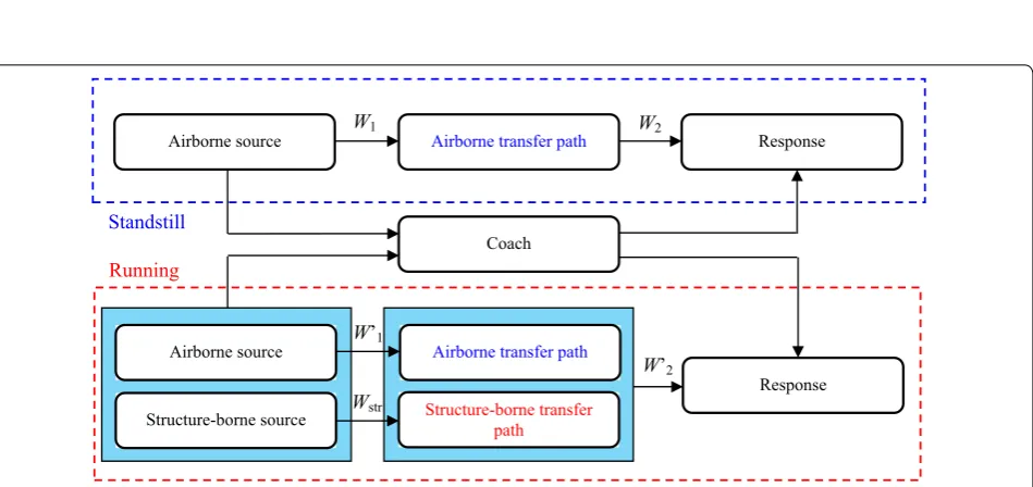
The exterior sound sources can contribute to the inte-rior noise through airborne and structure-borne transfer paths. Figure 11 shows sound transfer paths under differ-ent conditions.
(3)
L(v)=a×log10(v/v0)+L(v0),
Figure 8 Different areas at the end of the first coach
Figure 9 Contributions to the total sound power from different areas
Because the main interior noise sources at the end of the first coach are located at the sidewall and roof, we take the sidewall as an example. When the train runs at a constant speed, as shown in Figure 11(a), the sound
transferred through the sidewall includes both airborne sound and structure-borne sound. For high-speed trains, the coach is usually well sealed with negligible sound leakage; therefore, the airborne sound is transmitted from the exterior air environment to the coach (to excite structural vibration) and then to the interior air environ-ment, whereas the structure-borne sound is only trans-mitted from the coach structural vibration to the interior air environment.
When the train is stationary, and all equipment are shut down, there is no excitation. In that condition, if an airborne source is placed outside the train, as shown in Figure 11(b), there will be only airborne sound trans-ferred through the sidewall.
In addition, the airborne sound transfer path transmits the noise from the exterior sources facing the path at the sidewall, such as the bogie area noise and aerodynamic noise, whereas the structure-borne sound transfer path transmits the noise from the exterior vibration sources and related structural vibration propagation, such as the wheel and bogie frame vibrations.
60 70 110 120 130
Speed (km/h) Bogie area source Pantogarph area source Top area source Middle area source Bottom area source Interior noise
Bogie area noise
90 100 110 120 130
Sound Power Level (dBA
)
Sound Pressure Level (dBA
)
200 220 240 260 280 300 320 340 360
Figure 10 Relationships between the exterior noise and the interior
noise at different speeds
Table 1 Fitting results for the exterior and interior noises at different speeds
Interior noise Bogie area noise Bogie area
source Pantograph area source Top area source Middle area source Bottom area
source
a 33.5 31.6 27.6 40.0 31.3 32.4 24.0
L(v0) 63.0 113.0 118.2 109.6 113.2 117.8 117.7
R2 0.92 0.87 0.99 0.98 0.98 0.96 0.96
(a)
Running at a constant speed(b)
StationaryAirborne source
Structure-borne source
Structural vibration
Bogie area noise Bogie area vibration
Aerodynamic noise
Airborne source
Structural vibration
3.2 Method of the Transfer Contribution Analysis
Based on the description of the sound transfer path from the exterior to the interior, a method for analysing the con-tribution of airborne sound can be devised as shown in Figure 12.
The defined airborne sound transmission loss (or sound insulation) is Tair. From Figure 11(b), for a sidewall area with superficial area S, if the incident sound power from the exterior is W1, and the sound power transmitted to the interior is W2, Tair is given by
The defined structure-borne radiation sound power is Wstr. From Figure 11(a), the total sound power radiated by the sidewall is a sum of the airborne sound power and the structure-borne sound power. If the measured incident sound power is denoted by W′
1 , the transmission coefficient of the sidewall is τ, and the measured total sound power radiated by the sidewall is W′
2 , then
where
Therefore, from the measured airborne sound transmis-sion loss Tair when the train is stationary and the measured incident sound power W′
1 and total sound power radiated by the sidewall W′
2 when the train runs at a constant speed, the contributions of the airborne and structure-borne sound can be calculated as
(4)
Tair=10×log10(W1/W2).
(5) W2′=τW1′+Wstr,
(6) τ=10−0.1Tair.
(7)
Cair = τW ′
1
W′
2
= W
′
1W2
W′
2W1,
Cstr = WWstr′
2
=1−Cair,
where Cair and Cstr are the airborne and structure-borne sound contribution rates, respectively.
4 A Case Study of Noise from the Sidewall Area of the High‑Speed Train
4.1 Measurement and Analysis for the Stationary Condition
4.1.1 Measurement Configuration
When the train is stationary, the airborne sound trans-mission loss is measured by the sound intensity method near both sides of the sidewall. The selected sidewall area is at the coach end above a bogie. Due to the numerous windows on the sidewall, the selected area includes both a window and a part of the wall, as shown in Figure 13. The sidewall is 4 m from the gangway, and during the test both the inner end door and the gangway door are closed. This way, we ensure that the noise coming from the coach end has little influence. The dimensions of the sidewall are 1200 mm by 1200 mm, and those of the win-dow are 750 mm by 790 mm; thus, the winwin-dow accounts for 41% of the total area.
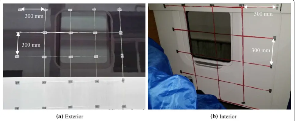
By integrating the sound intensity over a certain area, the sound power contributed by that area can be obtained. Therefore, we divide the studied area into a grid for measuring the sound intensity near the two sides of the sidewall as shown in Figure 14. In general, increasing the number of nodes in the grid leads to more accurate results. However, due to the limitations on the acquisi-tion time of the in-situ measurement, grid step is selected as 300 mm. Then, there are 25 nodes on each side of the sidewall. The sound intensities are measured at each node.
Airborne source Airborne transfer path Response
Airborne source Airborne transfer path
Response Coach
Structure-borne transfer path Structure-borne source
W1 W2
W’2 W’1
Wstr Standstill
Running
Two B&K Omni Power Sound Sources (B&K 4292-L) were placed inside the coach in order to obtain sufficient sound power and produce a close-to-reverberant sound environment. The two sources are independent and non-directional. White noise was used for excitation, with the upper frequency of 5000 Hz. Meanwhile, two sound intensity probes (B&K 3599) were used, one inside the coach and the other outside, to measure the sound inten-sities on the sidewall, as shown in Figure 15.
Before the measurement, the sound intensity probes were calibrated by the acoustic calibrator (B&K 4297). First, the sources were allowed to operate for 30 s to sta-bilise the sound environment, and then the sound inten-sity was measured for 30 s at each point on the grid.
4.1.2 Airborne Sound Transmission Loss Analysis
Figure 16 shows the measurement results for the sound intensity from the interior sidewall when the train is
stationary. The view direction is from the exterior to inte-rior. In addition to the values measured at the 25 points on the grid, values at other positions generated by linear interpolation with a step of 0.01 m are also shown. Fig-ure 17 shows the sound intensity results in the 1/3 octave bands.
It can be seen from Figure 16 that the sound inten-sity distribution on the interior sidewall is not uniform. There are higher levels on the upper part and lower lev-els on the middle and bottom parts. Although the sound sources had already radiated for 30 s before the sound intensity was measured, the acoustic field was still very complex, resulting in the differences in sound intensi-ties between different parts of the interior sidewall as large as 10 dB. These differences are likely related to the seats installed in the coach. The height of the seats cor-responds to the middle and bottom of the sidewall, and they have a shielding effect on sound propagation.
Figure 13 Test area of the sidewall of the high-speed train
From Figure 17, the average sound intensity spectrum from the 25 grid points shows a nearly straight hori-zontal line in the 1/3 octave bands centred from 100 Hz to 3150 Hz. However, the sound intensity levels in the 1/3 octave bands centred from 400 Hz to 1600 Hz are slightly lower than those in other bands. This is related to the sound absorption by the interior structures, such as seats and interior trim.
Figure 18 shows the measurement results for the sound intensity of the exterior sidewall when the train is stationary. The view direction is again from the exte-rior to inteexte-rior, and the overall spatial resolution is
0.01 m. Figure 19 shows the sound intensity results in the 1/3 octave bands.
It can be seen from Figure 18 that there are higher sound intensity levels on the left and right, and lower lev-els on the middle and bottom. The characteristics of the sound intensity distribution on the interior and exterior sidewalls are quite different. It is indicated that the noise from the airborne sound source transmitted through the sidewall not only defined by the characteristics of the source itself, but also affected by the structural character-istics and positions.
From Figure 19, the average sound intensity spectrum from the 25 points shows an obvious decreasing trend with increasing frequency, from 60 dB at 100 Hz to 20 dB at 4000 Hz. It shows that the noise from the air-borne sound source transmitted through the sidewall is frequency-dependent. In general, structures or materials have good acoustic performance with respect to param-eters such as sound insulation and sound absorption at high frequencies.
The distribution characteristics of the sound intensi-ties at both the interior and exterior sidewalls are related to the sound source excitation. Therefore, the airborne sound transmission loss must be considered to describe the noise transfer through the sidewall.
Since sound power is the integral of sound intensity over an area S, the airborne sound transmission loss can be expressed through the sound intensity as
where I1 and I2 indicate the incident and transmitted sound intensities for the area S, respectively.
(8) Tair=10×log10(W1/W2)=10×log10(I1/I2),
Figure 15 Photographs of the airborne sound transmission loss measurement
Figure 16 Sound intensity level of the interior sidewall (100–
Figure 20 shows the airborne sound transmission loss for the sidewall. The view direction is from the exterior to the interior.
From Figure 20, there are lower airborne sound trans-mission loss levels on the lower middle, upper right, and bottom right, and higher levels on the upper left, middle right, lower left, and lower right. The maximum variation of the airborne sound transmission loss of the sidewall in the tested region is about 10 dB. Lower losses mainly occur at the interface of the wall and window, espe-cially around the lower-left and upper-right corners. It is related to the structural installation characteristics and the lack of acoustic materials at the interface.
Because the measurement points on two sides of the sidewall are matched to each other and uniformly arranged, the areas of the grid cells can be considered equal. Then, the average airborne sound transmission loss of the entire measured sidewall can be calculated from the mean sound intensities on the two sides of the sidewall expressed as
where I1mean and I2mean are the average sound intensities inside and outside of the sidewall, respectively.
Figure 21 shows the average airborne sound transmis-sion loss of the sidewall as a function of frequency. The sound transmission loss increases with frequency, and its Rw (weighted sound reduction index) value is obtained as 42.4 dB. However, there are also some valleys in the 1/3 octave bands centred at 160 Hz and 630 Hz.
4.2 Measurement and Analysis for the Running Condition 4.2.1 Measurement Configuration
It is difficult to accurately measure the sound intensity outside the sidewall when the high-speed train is run-ning. Therefore, the sound intensity results outside the sidewall are obtained with the microphone array, whereas those inside the sidewall are still measured by a sound intensity probe. The measured area of the sidewall for the running train is the same as that for the stationary train. However, due to limitations arising from the experimen-tal conditions, the dimensions of the studied area of the sidewall in this measurement are 1000 mm × 1000 mm, whereas the number of the measurement points is still 25.
Figure 22 shows a photograph of the interior sound intensity measurement. The measurement begins when the train is running at a constant speed of 310 km/h. For each point, the sound intensity is acquired for 20 s.
4.2.2 Total Sound Power Radiation Analysis
Figure 23 shows the measurement results for the sound intensity of the interior sidewall when the train is
(9) Tair=10×log10(I1mean/I2mean),
100 200 400 800 1600 3150
50 60 70 80 90 100
Average
le
vel
yti
sn
etn
i
dn
uo
S
(
dB re 1pW/m
2)
Frequency (Hz)
Figure 17 Sound intensity spectrum of the interior sidewall
Figure 18 Sound intensity level of the exterior sidewall (100–
5000 Hz)
100 200 400 800 1600 3150
20 30 40 50 60 70
le
vel
ytis
net
ni
dn
uo
S
(dB re 1pW/m
2 )
Frequency (Hz)
Average
running at 310 km/h. The view direction is from the exte-rior to inteexte-rior. In addition to the values measured at the 25 points of the grid, values at other positions generated by linear interpolation are also shown, making the over-all spatial resolution 0.01 m. Figure 24 shows the sound intensity results in the 1/3 octave bands.
It can be seen from Figure 23 that there are high sound intensity levels inside the sidewall at the window and at the interface of the wall and window. Therefore, such areas radiate more noise from the exterior to the interior than other areas when the train is running at 310 km/h. The high noise level at the interface is related to the low airborne sound transmission loss, and the high noise level at the window is likely related to the dominant structural
vibration, as the window is associated with high airborne sound transmission loss.
From Figure 24, it can be seen that the sound inten-sity levels decrease as the frequency increases. There are peaks in the 1/3 octave bands centred at 125 Hz, 630 Hz, 1000 Hz, and 3150 Hz. These peaks correspond to the valleys in the airborne sound transmission loss levels (for example, the dip at 630 Hz in Figure 21) and the peaks in the exterior noise and vibrations.
Figure 25 shows the measurement result for the exte-rior noise sources of the first two coaches when the train is running at 310 km/h. The sidewall area outside is selected to be the same as that inside, and the sound power, which is equal to the average sound intensity in this case (as the area is 1 m2), is obtained, as shown in Figure 26.
From Figure 26, the sound intensity levels are around 90 dB in the 1/3 octave bands centred between 500 Hz and 3150 Hz. However, they decrease for frequencies above 2500 Hz. This is because the sidewall is located at the end of the coach; consequently, the levels are affected not only by the aerodynamic noise but also by the wheel/ rail rolling noise, with the rolling noise dominating in the 1/3 octave bands centred between 500 Hz and 2000 Hz [27].
4.3 Contribution of the Airborne Sound to the Interior Noise
For the selected sidewall area, using the sound intensity method and Eq. (7), we can calculate the contribution of the airborne sound to the interior noise in the following way:
where I1mean and I2mean are the average incident sound intensity and average radiated sound intensity, respec-tively, when the train is stationary. I’1mean and I’2mean are the average incident sound intensity and average radiated sound intensity, respectively, when the train is running at a constant speed. The results of the calculation according to Eq. (10) are shown in Figure 27.
From Figure 27, it can be seen that there is no particu-lar trend for the contribution rate as a function of fre-quency in the 1/3 octave bands centred from 500 Hz to 5000 Hz. However, the structure-borne sound dominates for the majority of the bands, whereas the airborne sound only shows a dominant contribution in the bands centred at 2000 Hz, 2500 Hz, 4000 Hz, and 5000 Hz. It is impor-tant to note that this behaviour is related to the charac-teristics of the airborne sound transmission loss of the coach. That is, because the airborne sound transmission (10)
Cair= I
′
1meanI2mean I′
2meanI1mean,
Cstr=1−Cair,
Figure 20 Airborne sound transmission loss of the sidewall
100 200 400 800 1600 3150
10 20 30 40 50 60
ss
ol
noi
ssi
ms
nar
t
dn
uo
S
(dB)
Frequency (Hz) Sidewall
Weighted sound reduction curve
Figure 21 Average airborne sound transmission loss of the sidewall
loss of the coach is sufficiently high to reduce the air-borne sound, the contribution from the structure-air-borne sound becomes dominant.
4.4 Discussion
It is necessary to point out that the above method may be more suitable for the aerodynamic effect on the sidewall surface is not significant. This is because aero-dynamic noise source near the sidewall has two compo-nents [28–30]: compressible acoustic pressure fluctuation and incompressible hydrodynamic pressure fluctuations, both exciting the wall to radiate noise inside the train. Due to the evanescent nature of the second component, the exterior noise estimated from microphone array measurement may only reflect the first component.
In response to this issue, we use a surface microphone fixed on the sidewall to measure the total pressure fluctu-ation. The contribution of airborne sound to the interior noise is reanalysed and compared with the previous one.
Figure 28 shows the measuring point of surface micro-phone on the sidewall outside. The surface micromicro-phone is installed at a height which corresponds to the centre-line of the window, and approximately 0.25 m from the left edge of the window. In general, more surface micro-phones lead to more accurate results. However, in order not to change the turbulent flow on the sidewall sur-face, the number of microphones should be kept to be minimum.
Figure 29 shows the sound pressure level outside the sidewall when the high-speed train was running at 310 km/h. The sound pressure levels decrease as the fre-quencies increase, and the levels are almost 90‒100 dB in the bands.
According to Eq. (10), the contribution of the airborne sound to the interior noise using sound pressure data can be expressed as
where p1mean and p2mean are average incident sound pres-sure and average radiated sound prespres-sure respectively when the train is stationary. p’1mean and p’2mean are aver-age incident sound pressure and averaver-age radiated sound pressure respectively when the train is running at a con-stant speed.
Figure 30 shows a comparison in airborne sound con-tribution results between microphone array and surface microphone.
It can be seen from Figure 30 that there are some dif-ferences of the airborne sound contribution results in frequency bands, especially in the 1/3 octave bands cantered at 1600 Hz, 2500 Hz and 4000 Hz. It is (11)
Cair= p
′2 1meanp2mean2
p′2 2meanp1mean2
,
Cstr=1−Cair,
Figure 22 Photograph of the interior sound intensity measurement
Figure 23 Sound intensity level of the interior sidewall (100–5000
Hz)
100 200 400 800 1600 3150
20 30 40 50 60 70 80
le
vel
yti
sn
etn
i
dn
uo
S
(dB re 1pW/m
2 )
Frequency (Hz)
Average
suggested to be caused by the incompressible hydro-dynamic pressure fluctuations on the sidewall surface. However, because the two curves are close in most bands, the incompressible hydrodynamic pressure fluc-tuations on the sidewall may have little influence in
this case. Nevertheless, it is still needed to do intensive study in the future
Furthermore, due to the experimental conditions, the contribution of the airborne sound to the interior noise is only investigated for the sidewall of a high-speed train. Even so, the method and obtained results are valuable for reference. At the same time, several issues remain and should be studied in the future. Here, we list some of them. First, in our measurement, when the train is stationary, the source is placed in the inte-rior, whereas when the train is running at a constant speed, the source is placed outside the coach. Here, it is assumed that the noise transmissions from the interior to the exterior and in the opposite direction are equiv-alent, which is not necessarily true in reality. Second, the sound field inside the coach is neither a free sound field nor a reverberation sound field. Thus, the effect of acoustic reflection in the measurement needs fur-ther investigation. Last but not least, the sound sources outside the sidewall are very complex. They include not only the aerodynamic noise and vibration, but also the bogie area noise and vibration. The accuracy of the measurements needs to be further verified.
5 Conclusions
This study investigates both the exterior and interior sound source distributions of a high-speed train and presents a method for the contribution analysis of the airborne sound to the interior noise. The conclusions are as follows:
1. When the high-speed train runs at 310 km/h, the main exterior sound sources are located at the bogie and pantograph areas. Here, the bogie area, mid-dle area of the coach, and bottom area of the coach provide dominant contributions to the total sound power.
2. When the high-speed train runs at 310 km/h, the main interior sound sources are located at the side-wall and roof. Here, the roof area provides the
maxi-Figure 25 Measurement results for the exterior noise sources (500–5000 Hz, Linear weighted)
500 1000 2000 4000
70 75 80 85 90 95 100
le
vel
yti
sn
etn
i
dn
uo
S
(
dB re 1pW/m
2)
Frequency (Hz)
Figure 26 Average sound intensity spectrum of the exterior sidewall
500 1000 2000 4000 10
30 50 70 90
eta
r
noi
tu
birt
no
C
(
%
)
Frequency (Hz) Airborne sound
Structure-borne sound
Figure 27 Contribution rate of the airborne sound to the interior
mum contribution to the total sound power, followed by the floor, right sidewall, and left sidewall areas. 3. The interior noise, the bogie area noise and the sound
source at the middle of the coach exhibit very similar rates of increase with increasing train speed. There-fore, the bogie area noise and the sound source at the middle of the coach contribute significantly to the interior noise.
4. For the selected sidewall area, the structure-borne sound dominates in the majority of the 1/3 octave bands, whereas the airborne sound dominates only in the bands centred at 2000 Hz and 2500 Hz. This behaviour is related to the characteristics of the air-borne sound transmission loss of the coach.
Authors’ Contributions
JZ put forward the method, analyzed the data and wrote the manuscript; XX and XS were in charge of the whole trial and reviewed the manuscript; ZL assisted with measurements and data analyses. All authors read and approved the final manuscript.
Authors’ Information
Jie Zhang, born in 1987, is currently a postdoctor at State Key Laboratory of Polymer Materials Engineering / Polymer Research Institute, Sichuan University, China. He received his PhD degree from Southwest Jiaotong University, China, in 2018. His research interests include railway noise and vibration.
Xinbiao Xiao, born in 1978, is currently an associate professor at State Key Laboratory of Traction Power, Southwest Jiaotong University, China. He received his PhD degree from Southwest Jiaotong University, China, in 2013. His research interests include railway noise and vibration.
Xiaozhen Sheng, born in 1962, is currently a professor and a PhD candi-date supervisor at State Key Laboratory of Traction Power, Southwest Jiaotong University, China. He received his PhD degree from University of Southampton, UK, in 2002. His research interests include railway noise and vibration.
Zhihui Li, born in 1988, is currently a research assistant at State Key Laboratory of Traction Power, Southwest Jiaotong University, China. He received his master degree from Southwest Jiaotong University, China, in 2016. His research interests include railway noise and vibration.
Acknowledgements
The authors sincerely thanks to Prof. Zhigang Chu (Chongqing University) and Associate Prof. Jianyue Zhu (Tongji University) for their critical discussion during the manuscript preparation, and thanks to Muxiao Li, Yumei Zhang, Moukai Liu, Rongchun Shi, Cai Tian, Yan Yang, et al. (Southwest Jiaotong Uni-versity) for their assistances in the measurements and data processing.
Competing Interests
The authors declare no competing financial interests.
Funding
Supported by National Key R&D Program of China (Grant No.
2016YFE0205200) and National Natural Science Foundation of China (Grant No. U1834201).
Received: 5 February 2018 Revised: 7 May 2019 Accepted: 2 July 2019
References
[1] A E J Hardy. Railway passengers and noise. Proceedings of the Institution of Mechanical Engineers Part F: Journal of Rail and Rapid Transit, 1999, 213(3): 173-180.
Figure 28 Photograph of the surface microphone installed on the
sidewall outside
500 1000 2000 4000
60 70 80 90 100 110 120
le
vel
er
uss
er
p
dn
uo
S
(
dB re 20uP
a
)
Frequency (Hz)
Figure 29 Sound pressure spectrum of the exterior sidewall
500 1000 2000 4000 10
30 50 70 90
eta
r
noi
tu
birt
no
C
(
%
)
Frequency (Hz)
Air-borne sound (using microphone array) Air-borne sound (using surface microphone)
Figure 30 A comparison in airborne sound contribution results
[2] N I Ivanov, I S Boiko, A E Shashurin. The problem of high-speed railway noise prediction and reduction. Procedia Engineering, 2017, 189: 539-546. [3] Z Y Shen. Dynamic environment of high-speed train and its distinguished
technology. Journal of the China Railway Society, 2006, 28(4): 1-5. (in Chinese)
[4] X S Jin. Key problems faced in high-speed train operation. Journal of Zhejiang University-Science A (Applied Physics & Engineering), 2014, 15(12): 936-945.
[5] G W Yang, Y J Wei, G L Zhao, et al. Research progress on the mechanics of high speed rails. Advances in Mechanics, 2015, 45: 201507. (in Chinese) [6] D J Thompson, P E Gautier. Review of research into wheel/rail rolling
noise reduction. Proceedings of the Institution of Mechanical Engineers, Part F, Journal of Rail and Rapid Transit, 2006, 220(4): 385-408.
[7] N Frémion, N Vincent, M Jacob, et al. Aerodynamic noise radiated by the intercoach spacing and the bogie of a high-speed train. Journal of Sound and Vibration, 2000, 231(35): 577-593.
[8] P J Remington. Wheel/rail rolling noise I: theoretical analysis. Journal of the Acoustical Society of America, 1987, 81(6): 1805-1823.
[9] D J Thompson. Wheel-rail noise generation, part 1: introduction and interaction model. Journal of Sound and Vibration, 1993, 161(1993): 387-400.
[10] T X Wu, D J Thompson. On the rolling noise generation due to wheel/ track parametric excitation. Journal of Sound and Vibration, 2006, 293(2006): 566-574.
[11] X Sheng, T Zhong, Y Li. Vibration and sound radiation of slab high-speed railway tracks subject to a moving harmonic load. Journal of Sound and Vibration, 2017, 395(2017): 160-186.
[12] X Zhang, D J Thompson, H Jeong, et al. The effects of ballast on the sound radiation from railway track. Journal of Sound and Vibration, 2017, 399(2017): 137-150.
[13] K Nagakura. Localization of aerodynamic noise sources of Shinkansen trains. Journal of Sound and Vibration, 2006, 293(2006): 547-556. [14] E Latorre Iglesias, D J Thompson, M G Smith. Component-based model to
predict aerodynamic noise from high-speed train pantographs. Journal of Sound and Vibration, 2017, 394(2017): 280-305.
[15] C Mellet, F Létourneaux, F Poisson, et al. High speed train noise emission: Latest investigation of the aerodynamic/rolling noise contribution. Jour-nal of Sound and Vibration, 2006, 293(2006): 535-546.
[16] E Zea, L Manzari, G Squicciarini, et al. Wavenumber-domain separation of rail contribution to pass-by noise. Journal of Sound and Vibration, 2017, 409(2017): 24-42.
[17] R Ström. Operational transfer path analysis of components of a high-speed train bogie. Sweden: Chalmers University of Technology.
[18] R Fan, Z Su, G Meng. Application of sound intensity and partial coherence to identify interior noise sources on the high speed train. Mechanical Systems and Signal Processing, 2014, 46(2014): 481-493.
[19] J Zhang, X B Xiao, X Z Sheng, et al. SEA and contribution analysis for interior noise of a high speed train. Applied Acoustics, 2016, 112(2016): 158-170.
[20] J J Christensen, J Hald. Technical review beamforming. Denmark: Bruel & Kjear, 2004.
[21] J Hald. Estimation of partial area sound power data with beamforming. INTER-NOISE and NOISE-CON Congress and Conference Proceedings, 2005. [22] Z G Chu, Y Yang. Comparison of deconvolution methods for the
visualiza-tion of acoustic sources based on cross-spectral imaging funcvisualiza-tion beam-forming. Mechanical Systems & Signal Processing, 2014, 48(1-2): 404-422. [23] J Zhang, X B Xiao, D W Wang, et al. Source contribution analysis for
exte-rior noise of a high-speed train: experiments and simulations. Shock and Vibration, 2018: Article ID 5319460.
[24] B He, X B Xiao, Q Zhou, et al. Investigation into external noise of a high-speed train at different high-speeds. Journal of Zhejiang University-Science A (Applied Physics & Engineering), 2014, 15(12): 1019-1033.
[25] B Rafaely. Plane-wave decomposition of the sound field on a sphere by spherical convolution. The Journal of the Acoustical Society of America, 2004, 116(4): 2149-2157.
[26] Z G Chu, Y Yang, Y S He. Deconvolution for three-dimensional acoustic source identification based on spherical harmonics beamforming. Jour-nal of Sound and Vibration, 2015, 344(2015): 484-502.
[27] D J Thompson. Railway noise and vibration: Mechanisms, modelling and means of control. New York: Elsevier, 2009.
[28] C Peric, S Watkins, E Lindqvist. Wind turbulence effects on aerodynamic noise with relevance to road vehicle interior noise. Journal of Wind Engi-neering and Industrial Aerodynamics, 1997, 69-71(1997): 423-435. [29] J Y Zhu, Z W Hu, D J Thompson. Flow simulation and aerodynamic noise
prediction for a high-speed train wheelset. International Journal of Aeroa-coustics, 2014, 13 (7&8): 533-552.