The Thirty-Third AAAI Conference on Artificial Intelligence (AAAI-19)
Human-in-the-Loop Feature Selection
Alvaro H. C. Correia
∗ENSTA ParisTech, Palaiseau, France Utrecht University, The Netherlands
Freddy Lecue
∗CortAIx Thales, Montreal, Canada Inria, Sophia Antipolis, France
Abstract
Feature selection is a crucial step in the conception of Ma-chine Learning models, which is often performed via data-driven approaches that overlook the possibility of tapping into the human decision-making of the model’s designers and users. We present ahuman-in-the-loopframework that inter-acts with domain experts by collecting their feedback regard-ing the variables (of few samples) they evaluate as the most relevant for the task at hand. Such information can be mod-eled via Reinforcement Learning to derive a per-example fea-ture selection method that tries to minimize the model’s loss function by focusing on the most pertinent variables from a human perspective. We report results on a proof-of-concept image classification dataset and on a real-world risk classi-fication task in which the model successfully incorporated feedback from experts to improve its accuracy.
Introduction
Selecting a subset of the available features for a given Ma-chine Learning task, also known asfeature selection, is a critical step that helps in the design of relevant, accurate and robust models (Guyon and Elisseeff 2003; Chandrashekar and Sahin 2014). Although ideally models should be capa-ble of identifying the most predictive features during train-ing, a large input space can reduce performance due to the “curse of dimensionality”: the amount of data required to fit a reliable estimator increases exponentially with the number of variables. Therefore, a model based on a smaller number of features might produce better results while being faster and more cost-effective.
A way of tackling this problem is to select features ac-cording to experts’ prior knowledge, but that is costly, time demanding and manual. Furthermore, often the users with the relevant understanding of the domain and task are not the ones designing the model. An alternative is to resort to methods that automatically rank and select features under some measure of relevance or importance. Even so, a limi-tation common to manual and automatic approaches alike is that they define a single feature subset to represent the entire dataset. When the amount of training data is small compared to the number of features, a single subset is unlikely to be
∗
Work funded by Accenture Labs, Ireland for an internship. Copyright c2019, Association for the Advancement of Artificial Intelligence (www.aaai.org). All rights reserved.
able to describe all observations (Avdiyenko, Bertschinger, and Jost 2012).
Towards this challenge, we present aper-example feature selection method by including the human-in-the-loop. We propose a framework where experts are asked to identify the most relevant features for a few examples. Reinforcement Learning (RL) allows us to use that feedback to explicitly model the probability of selecting each feature and derive a policy that produces a new feature subset for each observa-tion in the dataset. Each example is thus represented by a different set of features, which is the only input to a subse-quent learning algorithm (e.g., a classifier or regressor). The feature selection policy is learned through policy gradient methods to minimize both (i) the loss function of the asso-ciated learning algorithm and (ii) the dissimilarity between the feature subsets chosen by the model and the users.
Such an approach can not only improve the performance of the model but also render its decision-making more inter-pretable to human users. As the final prediction relies only on the selected feature subset, which is individual to each example, one can interpret those variables as an explanation for the model’s output. Moreover, by mimicking human an-notation in selecting the most relevant features, the model can better reflect causal relationships in the experts’ minds.
We frame our model as a stochastic computation graph (Schulman et al. 2015) and compare two different solvers: Score Function (SF) and Pathwise Derivative (PD) estima-tors. We validate our method in two scenarios: (i) a proof-of-concept image classification task and (ii) a real-world project risk classification task. In the latter, which is highly human-curated, our architecture improves the baseline ac-curacy by more than 50%. We also study the influence of different hyperparameters and factors of practical relevance, such as the required number of pieces of feedback and the presence of conflicting information from different experts.
The next section reviews related work. Then, we present (i) the feature selection problem, (ii) our human-in-the-loop approach, (iii) the stochastic computation graph framework with the SF and PD solvers, and finally (iv) the experiments in the two tasks described above.
Related Work
Sahin 2014) for excellent surveys. More precisely, we are concerned with variable elimination techniques, where only a subset of the available features is selected. These are tradi-tionally divided infilters(Tyagi and Mishra 2013),wrappers
(Kohavi and John 1997) andembeddedmethods (Guyon and
Elisseeff 2003). Filter methods consist of a preprocessing
step where the top-k features are selected by ranking them against some score function, such as the mutual informa-tion between input and target variables. Conversely,wrapper methodsrank feature subsets following some performance measure such as the accuracy in the training data. That re-quires retraining the model for each candidate subset, which can be computationally costly and time-consuming. Finally,
embedded methodstry to solve that problem by performing feature selection while training the learning algorithm.
Our approach can be classified as an embedded method because we jointly train the feature selection and the learn-ing algorithm via gradient descent. However, it distlearn-inguishes itself from conventional ones because it selects a differ-ent subset of the features for each observation. Such a per-example approach can better describe the data (Avdiyenko, Bertschinger, and Jost 2012) and render the output more in-terpretable, as the selected variables can be understood as the “causes” that drive the model’s decision-making.
Per-example feature selection has also been studied in (Avdiyenko, Bertschinger, and Jost 2012). They proposed a filter method based on the mutual information between fea-tures and target variables, conditioned on the specific val-ues of each example. The mutual information is then used as a score to rank thekmost relevant features for each in-put. Their work contrasts with ours in two significant ways: (i) their method is deterministic and completely data-driven, whereas ours include human feedback to provide insights that cannot be automatically inferred from small or com-plex datasets; (ii) they build a subset sequentially, while our method produces a candidate subset in a single step, with no need for an arbitrary stop criterion.
Our model is also inspired by recent developments in
attention mechanisms in deep learning (Mnih et al. 2014; Xu et al. 2015; Bengio, L´eonard, and Courville 2013; Bahdanau, Cho, and Bengio 2015). By attributing weights to the different hidden states in a neural network, attention mechanisms are also selecting the most relevant features to minimize the model’s cost function. Our contribution lies in the application of such attention mechanisms to human-in-the-loop architectures as a way to provide prior knowledge to the model on-the-fly.
Finally, our model also relates to probabilistic approaches to knowledge elicitation (Cano, Masegosa, and Moral 2011; House, Leman, and Han 2015; Daee et al. 2017). The work by Daee et al. is particularly relevant because they also query users about feature importance. However, they only model global feature relevance, whereas we propose a per-example feature selection method capable of eliciting the variables that drive the prediction for each observation.
Feature Selection
We assume a supervised learning scenario, where a para-metric model is trained to minimize some cost function
C(x, y, θ), wherexis the input,yis the target, andθis the set of parameters defining the model. For clarity, we refer to the model’s prediction asyˆto contrast with the true valuey.
Framework
We propose a framework where the annotators or the users not only provide the ground truthybut also select the most relevant features for some of the examples in the dataset. That is common practice when experts emphasize some characteristics of the data to drive the machine learning modeling (Raghavan, Madani, and Jones 2006). To model that annotation and perform feature selection (variable elim-ination) on a per-example basis, we introduce a maskathat is applied over the input vectorxto filter out irrelevant fea-tures in each observation. Therefore, if an example is given
byx∈ Rd, where each dimension corresponds to a feature
xj, thenais an indicator variable in{0,1}d, such that:
a
j = 1, ifxjis used for examplex
aj = 0, otherwise.
(1)
We denote the input to the learning algorithm byx0, which
is now given byx0 =xa, whereis the element-wise
or Hadamard product. As the feature selection is performed
on a per-example basis,a must be a function of the input
x. However, ifais an indicator variable, we cannot apply gradient descent to minimize the lossC(x0, y, θ)because it is no longer differentiable with respect to the function that definesa. For that reason, we make variableastochastic and model the probability ofaconditioned onx. Given thata∈ {0,1}d, we can associate each componenta
jto a Bernoulli
distribution parametrized byqˆjand obtain:
π(a|x) =
d
Y
j=1
ˆ
qaj
j (1−qˆj)(1−aj). (2)
Our objective is to concentrate the mass of the distribu-tionπ(a|x)on values ofathat minimize the loss function C(x0, y, θ). To achieve that, we will resort to RL and, in par-ticular, policy gradient methods (Sutton and Barto 2011). Hence, we will refer to π(a|x) as a policy, which should tell us the bestagiven the current inputx. Keeping the RL jargon, the function that defines such a policy will be called an agent. The probabilityqˆj of each feature being selected
by this agent will be a function of xand approximated by
a neural network with parameters ψ, where the last layer
consists of a sigmoid function to squash the results into a
probability space. The vector composed of alldparameters
ˆ
qjis estimated in a single step by this neural network.
ˆ
qψ= (ˆq1,qˆ2, ...,qˆd) =h(x;ψ). (3)
π(a|x) =
d
Y
j=1
K Y
k=1
ˆ
qjk[aj=k], (4)
whereqˆjkis the probability of assigning statekto featurej
and[aj =k]evaluates to 1 ifaj=k, 0 otherwise.
Human-Like Feature Selection
The framework described above can also be used to model the feature selection performed by humans. We will assume without loss of generality that the annotators’ feedback can be translated into a vectorq ∈ [0,1]d, where each element
qjreflects the importance attributed to featurej. In that case,
qis directly comparable to the model’s outputqˆ, which can also be interpreted as the relevance of each feature. The intu-ition is that ifqjorqˆjis close to one, featurejis determinant
to predictyˆand is negligible otherwise.
Therefore, to train the agent to mimic the feature selection done by the users, first we need to define a similarity mea-sure betweenqandqˆ. The distance betweenqandqˆis also a cost function, which we will refer to asCf(x, q, ψ)in (5)
to distinguish it fromC(x0, y, θ). The Euclidean distance is a straightforward option of a distance measure, which results
Cf(x, q, ψ) =Ex||qi−qˆi||2=Ex||qi−h(x;ψ)||2. (5)
The Mean Squared Error (MSE) betweenqandqˆ, as
de-fined above, is not the only possibility, and other dissimilar-ity functions might be pertinent depending on the applica-tion and type of feedback. For instance, an alternative is the cosine distance
Cf(x, q, ψ) = 1−
qqˆ
||q||2||qˆ||2
= 1− q h(x;ψ) ||q||2||h(x;ψ)||2
. (6)
With the cosine distance, we penalize the agent if the two vectors do not have the same orientation in space but ignore differences in magnitude.
Once the similarity measure is defined, we just have to addCf(x, q, ψ)to the final cost function to which we will
refer asCin (7) to simplify the notation.
C=C(x, y, q, θ, ψ) =C(x0, y, θ) +λCf(x, q, ψ). (7)
That can be interpreted as the sum of two reward signals that encourage the agent to achieve a good performance at the machine learning task while mimicking human feature se-lection. In (7)λis a hyperparameter that balances the trade-off between these two signals. Such sum of errors for differ-ent tasks is common practice in multi-task learning (Caruana 1997) Note that the framework does not require human fea-ture selection data to be provided for all data. For examples with no available feedback,Cf(x, q, ψ)is set to zero.
Stochastic Computation Graphs
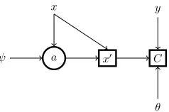
The maskais stochastic and before making a prediction, we first need to sampleafrom the policy defined in (2). Hence, we can frame the whole model, including the feature selec-tion and the learning algorithm, as a stochastic computaselec-tion graph (Schulman et al. 2015). That allows for a straightfor-ward comparison of possible solvers and clear representa-tions of the model as depicted in Figures 1 and 2.
a ψ
x
x0 C
θ y
Figure 1: Stochastic graph for the score function estimator. As in (Schulman et al. 2015), square nodes are deterministic, whereas round ones are stochastic. Inputs and parameters are represented by their corresponding vector names.
The challenge in a stochastic computation graph is that the standard backpropagation algorithm is no longer suffi-cient because the cost C(x0, y, θ)is non-deterministic and non-differentiable with respect to the parametersψ. In that case, we need some way of estimating∇ψEa[C], the
gra-dient of the expected loss function with respect to the policy parameters. To that end, we can resort to one of the follow-ing estimators to find the optimal policyπ(a|x): (i) theScore Function(SF) and (ii) thePathwise Derivative(PD) estima-tors (Schulman et al. 2015).
Score Function Estimator
The Score Function estimator (SF), also known as the RE-INFORCE algorithm (Williams 1992), consists in rewriting ∇ψEa[C] as Ea
h
C ∇ψlog π(a|x, ψ)
i
. Practically, it
al-lows the complete model to be trained by gradient descent to minimize a surrogate cost functionC0defined as follows:
C0 =Clog π(a|x, ψ)+C. (8)
In many cases, it is desirable to favor a subset with a smaller number of features, even if that does not decreaseC0. To encourage the desired sparsity in the maska, we follow the approach used in (Bengio et al. 2016) and introduce a regularizerLs, which penalizes the model ifqˆjis not sparse.
Ls=E
h (||1
d
d
X
j
ˆ
qj)−φ||2
i
, (9)
whereφ∈[0,1]is an hyperparameter that specifies the de-sired sparsity of activation. We also wantqˆto have high vari-ance across different examples to avoid always selecting the same subset of features. Hence, we add another regularizer to penalize low variance across examples in the same batch.
Lv =− d
X
j
1
m
m
X
i
ˆ
qij−
1
m
m
X
i
ˆ
qij
2
, (10)
where the indexirefers to each examplexandmis the batch
size. The model is then trained to minimizeC0 +λ
sLs+
λvLv, where λs andλv are hyperparameters that balance
Pathwise Derivative Estimator
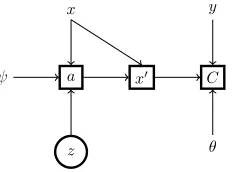
The second alternative is to use the Pathwise Derivative es-timator (PD), which is also known as the reparametrization trick and was made popular by variational autoencoders in-troduced in (Kingma and Welling 2014). We can sample from π(a|x) by first sampling a latent variable z from a known fixed probability distributionp(z)and transforming it using some function to recovera. In that case, the mask
ais no longer sampled from a random variable because we
introduce another stochastic nodez to account for the ran-domness in the process. The corresponding graph for the pathwise derivative estimator is shown in Figure 2.
a
z ψ
x
x0 C
θ y
Figure 2: Stochastic graph for the pathwise derivative esti-mator. Here the maskais no longer a stochastic node.
In variational autoencoders, z is usually distributed ac-cording to a Gaussian distribution (Kingma and Welling 2014; Kingma et al. 2016), but the reparametrization trick can be extended to categorical variables by samplingzfrom a Gumbel-softmax distribution (Jang, Gu, and Poole 2017; Maddison, Mnih, and Teh 2015). To use that distribution, we first need to rewriteaas a one-hot vector to match the out-put of a softmax. AssumingKdifferent possible states,ajk
is the probability of assigning statekto featurej, which can be calculated as
ajk=
exp((log(ˆqjk) +gk)/τ)
PK
l=1exp((log(ˆqjl) +gl)/τ)
for k in 1, ...,K,
(11) whereg0, g1, ..., gk, are samples from Gumbel(0,1)
(Gum-bel 1954) andτis a hyperparemeter that defines how close
the distribution is from the argmax function. For τ > 0,
equation (11) is smooth and differentiable, but for τ = 0
it is simply an argmax function. Hence, during trainingτ is maintained positive, but we gradually decrease its value as the model approaches convergence. During test time, we do not need the cost function to be fully differentiable andτis set to zero to recover an argmax function.
Now the mask is a matrix a ∈ Rd×K and we need to
reduce it to a vector of sizedbefore multiplying it by the in-putx. One way to do so is to multiplyaby a set of weights
w ∈ RK, so thataw ∈ [0,1]d. For instance, if we want to parametrize a Bernoulli distribution as in (2),ajwould have
two states andwwould be[0,1]T. Note that forτ >0,ais
no longer an indicator variable, but is continuous in the inter-val[0,1]. That is a relaxation that renders the graph wholly differentiable during training, but we regain the original def-inition ofain (1) during test time whenτ= 0.
The advantage of the pathwise derivative estimator is that
it does not require a surrogate cost function and we can up-date the whole model via gradient descent by minimizing (7). We also observed that the PD estimator does not require the same type of regularization as the SF estimator, which re-duces the number of hyperparameters that need fine-tuning. However, it does introduce another hyperparameter for the
temperature τ, so that the entropy in the Gumbel-softmax
can be regulated during training.
Experimental Results
We validate our feature selection method on: (i) a proof-of-concept image classification task for reproducibility and (ii) a real-world project risk classification task. All exper-iments were developed on top of the Tensorflow python API (GoogleResearch 2015) and run on a single GPU Nvidia GEFORCE GTX 1080 Ti. The code for the image classification task can be found at github.com/AlCorreia/ Human-in-the-loop-Feature-Selection.
Set-up: The architecture of our feature selection model is similar for both use cases, which shows the generality of our approach. The classifier was a neural network with a feedfor-ward architecture and a hidden layer of 256 neurons. The last activation was a softmax to yield the negative log-likelihood used as loss function for the classification task. The RL agent was also neural network-based with a single hidden layer of 128neurons. In both cases, the activation function between the layers was a rectified linear unit (ReLU). For the project risk classification dataset, categorical features were embed-ded in a vector of sizelog2nwherenis the total number of categories. These embeddings were learned via backpropa-gation with the rest of the model.
Runs: The model based on the PD estimator was trained
for 100 epochs with batches of 876 projects (1000
im-ages), but the feedback was only provided during the last
50epochs. The SF estimator was trained the same way, but
as it proved noisier, we also pretrained the network without any feature selection for40epochs. In each training phase, the whole model was updated via Adagrad (Duchi, Hazan, and Singer 2011) with initial learning rate of.5. The hyper-parameterλin (7) was set to1, so that minimizing the cost function and reproducing the feedback were equally impor-tant objectives. For the SF estimator, the regularization pa-rametersφ,λsandλv in (9) and (10) were set to.2,1and
1, respectively. For the PD estimator, different values for the temperature parameter were tested, but for the results in
Ta-ble 4 and 5, it was set to10and decayed by4%every100
steps to slowly render the model more deterministic.
Image Classification Task
To prove that the agent can select relevant features, the attention vector was equally applied over all the filters of the convolution to make the mask directly related to locations in the image. Thus, one can interpret whether the agent’s selection was pertinent by visually comparing it against the actual position of the digit.
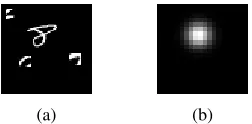
Feedback Computation: We simulated user feedback by fitting a 2D Gaussian with the position of the center of the digit for the mean. All training data was generated on-the-fly by repeating the above process. The test data was com-posed of a fixed set of 5000 images produced in the same way. Figure 3 shows an example of a cluttered image and its corresponding feedback.
(a) (b)
Figure 3: Cluttered MNIST image and simulated feedback.
Baseline: The baseline for the experiments is given by the neural network with the same architecture, but without any feature selection, i.e. all the features extracted by the convo-lutional layer are fed to the classifier. That model was able to classify correctly 92.23% of the examples in the test set after 100 epochs with batches of 1000 examples.
Selected Features: Figure 4 shows the evolution of the probabilitiesqˆcorresponding to Figure 3, during the train-ing of the model with the PD estimator. The model gradually learned to focus on a single region of the image, butqˆonly became sharp after the feedback was introduced.
(a) Beginning (b) 25 epochs (c) 50 epochs (d) feedback
Figure 4: Evolution of the probabilities vectorqˆduring train-ing of the model with PD estimator and MSE feedback.
Comparing Estimators
Table 1 shows the results obtained with both estimators when applying the proposed feature selection method on a cluttered MNIST dataset with a frame of 60x60.
Table 1: Estimators Impact on Accuracy (%).
Feedback / Estimator SF PD
Before Feedback 85.35 85.70
Cosine Feedback 92.30 88.40
MSE Feedback 91.16 89.61
Both estimators produced similar results during the first phase when the feature selection was based on the classifi-cation cost only. Despite similar performances, the PD esti-mator has the advantage of not requiring pretraining nor any regularization or variance reduction parameters.
In both cases the inclusion of the simulated feedback pro-duced a considerable improvement in the accuracy of the model. However, the SF estimator proved more efficient in incorporating the human feature selection, outperforming the PD estimator by almost 5%. The difference can be at-tributed to the difficulty in fine-tuning the hyperparameter
τ for the PD estimator based on the Gumbel-softmax. Even
though the temperature was decayed during training,τ was
probably still too high to allow for an efficient integration of the feedback. As indicated by the experiments presented in the next section, forτaround1.0the PD estimator produces similar results to those obtained with the SF here.
Impact of Temperature on Accuracy
The temperatureτ is the only hyperparameter that needs to
be fine-tuned when solving the graph with the PD estima-tor. We ran the model with the same architecture described above, but with five different values for the temperature. Dif-ferently from the previous experiments, in this case the value ofτwas kept constant during the whole training.
Table 2: Temperature Impact on Accuracy (%).
Temperature Value Before feedback After feedback
0.25 84.77 88.70
0.50 85.48 89.76
1.0 86.5 91.20
3.0 84.10 88.90
10.0 84.77 88.82
When τ is close to zero, the Gumbel-softmax approaches
an argmax over the probabilitiesqˆj, which means the agent
only exploits and always picks the value fora that
maxi-mizes the reward under its current policy. For τ > 0, aj
becomes stochastic, which allows the agent to explore and observe the loss for intermediate values ofa. However, ifτ
is high, equation (11) is close to an uniform distribution over itsKcategories andajkis K1 for everyk. Hence, assuming
a fixed set of weightsw, the final value forajwould remain
constant and independent of the policy parameters ψ,
pre-venting the agent from updating its policy effectively. That is reflected in the results presented in Table 2. A temperature value of1.0produced the most accurate model, presumably striking a balance between exploration and exploitation.
From Bernoulli to Categorical Distribution
the feedback and achieved similar accuracy values to those presented Table 1. One can also conclude that the feedback is all the more valuable when the search space is large.
Table 3: Number of States on Accuracy (%).
States Before Feedback Cosine MSE
2 85.15 88.40 89.50
3 83.82 88.70 89.61
10 80.83 88.69 88.98
20 74.24 86.62 85.40
Project Risk Classification Task
Business Context: We experimented our feature selection
method on a Project Risk Classification (PRC) dataset. 4
years of project risk profiles of a leading service company, capturing349,324 projects across97features (19
categor-ical and 78 numercategor-ical) and classified among 5 categories
(from high to no financial risk) are captured.
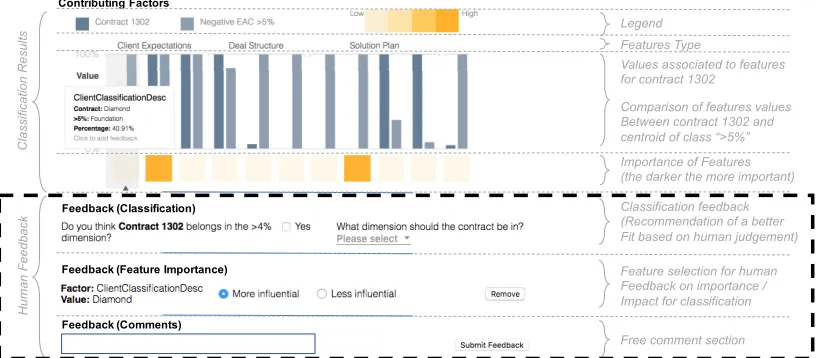
During the feedback collection phase, 114 business
ex-perts contributed by informing on: (i) (recommended) class, (ii) important features, (iii) textual comments (manually used to filter out some cases) cf. Figure 5. A total of613,916 pieces of feedback on87,657active contracts (their classi-fication and important features) have been collected over a
6-month pilot with an average of7 pieces of feedback per
project, and45per person/day. On average, the business ex-perts provided feedback on11 (standard deviation of 3.9) variables per example. Naturally, some feedback is conflict-ing among users:21.6%(resp.12.8%) of the feedback con-flict at class (resp. feature importance) level.
Motivation: The PRC problem fits our framework as (i) baseline approaches reach a (low) maximum accuracy of 31.45% (random forest), (ii) project risk assessment is a highly human-curated task where experts can expose their knowledge by identifying relevant features, and (iii) com-pletely data-driven approaches would require large amounts of data given the sparsity inherent of this context.
Feedback Computation: From now on, we will use the term feedback to refer to the feature-level annotation only, as we are mostly interested in feature selection. We limited the feedback to the binary impact of each feature because it facilitates the labeling task and better correlates with our variable elimination framework. Therefore, for each obser-vation i, a piece of feedback translates to a binary vector
qi ∈ {0,1}d, whereqi,j = 1iff featurejis relevant for
ex-amplei. Each exampleireceived feedback from an average
of7users. Consequently, for all experiments except those on Table 7, eachiappeared multiple times in the dataset with differentqi’s. All those observations were treated
indepen-dently and randomly selected during training.
Validation: Accuracy is measured by comparing the pre-dicted risk class with the real-world observations of risk for completed projects. Training, testing and validation sets cor-respond to 60/20/20% of the projects, respectively, with each class equally distributed in the validation and test sets.
Baseline: There are two baselines for the experiments: (i) a random forest trained with the same features, which
at-tained accuracy of 31.45% and (ii) a neural network with
the same architecture described above (cf. Technical Context set-up), but without any feature selection. The latter classi-fies correctly29.01%of the examples in the test set after 100 epochs with batches of 876 examples.
Selected Features: After training with the feedback, the model selected a relatively low number of features: 2 to 12 (mean: 4.6, std: 1.5). Such a low number of selected features is desirable as it favors the interpretability of the model.
Impact of Estimators on Accuracy
Table 4 reports the accuracy obtained with SF and PD esti-mators when applying our method on the PRC dataset.
Table 4: Accuracy (%) on PRC Test Set with Each Estimator.
Feedback / Estimator SF PD
Before Feedback 29.53 29.99
Cosine Feedback 82.49 77.51
MSE Feedback 80.11 78.44
The results show a very similar pattern to the one ob-served in the image classification dataset. Once more the SF
was superior by5%, but the PD was slightly more accurate
before the introduction of feedback.
Impact of Temperature on Accuracy
We also varied the temperatureτ for the PD estimator on
the PRC dataset. The results presented in Table 5 support the same conclusions we reached on the image classification task. Aτof1.0lead to a higher accuracy both before and af-ter the introduction of feedback, which suggests that would be a good defaultτvalue for the PD estimator.
Table 5: Temperatures on Accuracy on PRC (PD & MSE).
Temperature Value Before feedback After feedback
0.25 28.78 77.82
0.50 30.02 78.77
1.0 31.15 81.87
3.0 27.98 78.33
10.0 28.36 78.07
Feedback Impact on Accuracy
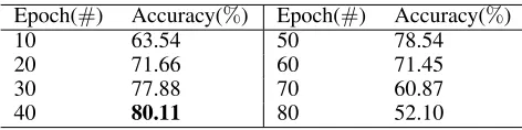
Qualitative Feedback Impact (1): Table 6 presents an analysis of the optimal moment to start injecting the feed-back into the model solved with the SF estimator. Even though pre-training the network without any feature selec-tion is beneficial, feedback should be provided no later than 40epochs into the training phase to reach optimal results.
Table 6: Feedback epoch on Accuracy on PRC (SF & MSE).
Epoch(#) Accuracy(%) Epoch(#) Accuracy(%)
10 63.54 50 78.54
20 71.66 60 71.45
30 77.88 70 60.87
Feedback (Classification) Contributing Factors
Feedback (Feature Importance)
Feedback (Comments)
Importance of Features (the darker the more important) Values associated to features for contract 1302
Comparison of features values Between contract 1302 and centroid of class “>5%” Features Type
Free comment section Feature selection for human Feedback on importance / Impact for classification Classification feedback (Recommendation of a better Fit based on human judgement)
H
um
an
F
ee
db
ack
C
la
ssi
fica
tio
n
R
esu
lts
Legend
Figure 5: User interface for Project Risk Classification problem (human feedback collection inside dashed zone).
Qualitative Feedback Impact (2): We run the same tests with4,8, 16and 32states cf. Table 7 to evaluate the in-fluence of the number of statesKon the performance of the PD estimator. To match these different numbers of states, we combined the input from multiple users into a single score per example,qi∈ {0,161, ...
15
16,1}(16is the max. number of
reviews per example). That score was adjusted proportion-ally to match the other versions with2,4,8and32states.
Table 7: Accuracy (%) on PRC Test Set with PD Estimator on Different Number of States.
States Before Feedback Cosine MSE
2 24.01 72.99 73.11
4 29.53 77.00 77.51
8 28.71 79.21 79.44
16 26.39 78.01 78.33
32 26.14 76.17 76.24
The accuracy of the model increases with the number of
states up toK = 8(outperforming results in Table 4) and
then decreases. Although the search problem grows in plexity with the number of states, that seems to be com-pensated by the more fine-grained feedback. However, for
K > 8 the model starts to underperform, which indicates
that at that point the number of pieces of feedback available is no longer enough to offset the larger search space. These results contrast with the ones shown in Table 3, as the more complex PRC dataset benefits more from granular feedback.
Quantitative Feedback Impact (1): As 12.8% of the feedback is conflicting among users, we evaluated the im-pact of such conflicts in Table 8. We varied this ratio by removing any conflicting feedback up to the point of not having any conflicts cf. case0. We only removed pieces of feedback which had no common basis, qi,j 6= q0i,j∀j.
In-terestingly, the best result was obtained when including6% of the conflicting feedback. Although counterintuitive, such feedback might relax the constraint on some features, free-ing the model to focus on minimizfree-ing the classification error.
Table 8: Conf. Feedback on Accuracy on PRC (SF & MSE).
Number (#) Conf. Feedback (%) Accuracy (%)
864,393 12.8 80.11
607,776 9 84.56
405,184 6 86.67
202,592 3 78.89
0 0 69.87
Quantitative Feedback Impact (2): Table 9 reports the impact of the quantity of feedback, considering similar ratio of conflicting feedback as for Tables 4 and 5. The accuracy plateaus with80%of feedback. Thus, an average of5.6 com-ments per project is required to obtain77.54%of accuracy, which above the goal set up by the project stakeholders.
Table 9: Feedback Size on Accuracy on PRC (SF & MSE).
Feedback Size(#) Feedback Ratio(%) Accuracy(%)
0 0 29.53
3,376,538 50 61.65
5,402,460 80 77.54
6,077,768 90 78.11
6,753,076 100 80.11
Lessons Learnt
We learned a few important characteristics of the proposed human-in-the-loop architecture:
1. We observed the SF estimator does not respond well to dropout (Srivastava et al. 2014). Conversely, the PD es-timator seems to benefit from this type of regularization (we used a dropout rate of0.8for all PD experiments);
2. The architecture used to model the agent is independent of the estimator. One can change between them during training to take advantage of both methods;
Conclusion and Future Work
We address the problem of human-in-the-loop per-example feature selection as a stochastic computation graph. It is a general approach that can be applied to a variety of machine learning tasks with little modifications, as demonstrated by the very distinct datasets we tackled in this paper. Direct ap-plications could be in the context of transfer learning (Chen et al. 2018). With the image classification dataset, we visu-ally proved the model can identify the most relevant features of each example, even though in that simple task, that did not reflect in a gain in accuracy. With the PRC dataset, we showed that our model successfully employed real human feedback to produce a significant improvement in accuracy, while also providing business-driven insights to the users. Most importantly, this new architecture enables a symbi-otic interaction with stakeholders as the feature selection not only can enhance the model performance but also inform the most relevant properties of each example to the users. Thus, this type of interaction might prove useful in further devel-opments of explainable artificial intelligence.
We identify two main lines of research for future work. The first is to extend the architecture to the full active learn-ing scenario, where the model asks the users about specific examples. The second is to model the dependence between the features explicitly via a prior distribution over the proba-bilitiesqˆor a more complex RL policy. We framed the model as an RL problem precisely to support extensions of this sort.
References
Avdiyenko, L.; Bertschinger, N.; and Jost, J. 2012. Adaptive Se-quential Feature Selection for Pattern Classification. InIJCCI In-ternational Joint Conference of Computational Intelligence, 474 – 482.
Bahdanau, D.; Cho, K.; and Bengio, Y. 2015. Neural Machine Translation By Jointly Learning To Align and Translate. Interna-tional Conference on Learning Representations 2015.
Bengio, E.; Bacon, P.-l.; Pineau, J.; Precup, D.; Networks, K. N.; and Computing, C. 2016. Conditional computation in neural net-works for faster models. InInternational Conference on Learning Representations, Workshop Track, ICLR 2016.
Bengio, Y.; L´eonard, N.; and Courville, A. 2013. Estimating or Propagating Gradients Through Stochastic Neurons for Con-ditional Computation.arXiv:1308.34321–12.
Cano, A.; Masegosa, A. R.; and Moral, S. 2011. A method for in-tegrating expert knowledge when learning bayesian networks from data. IEEE Transactions on Systems, Man, and Cybernetics, Part B (Cybernetics)41(5):1382–1394.
Caruana, R. 1997. Multitask learning. Machine Learning 28(1):41–75.
Chandrashekar, G., and Sahin, F. 2014. A survey on feature selec-tion methods. Computers and Electrical Engineering40(1):16– 28.
Chen, J.; L´ecu´e, F.; Pan, J. Z.; Horrocks, I.; and Chen, H. 2018. Knowledge-based transfer learning explanation. InPrinciples of Knowledge Representation and Reasoning: Proceedings of the Sixteenth International Conference, KR 2018, Tempe, Arizona, 30 October - 2 November 2018., 349–358.
Daee, P.; Peltola, T.; Soare, M.; and Kaski, S. 2017. Knowl-edge elicitation via sequential probabilistic inference for high-dimensional prediction. Machine Learning106(9):1599–1620. Duchi, J.; Hazan, E.; and Singer, Y. 2011. Adaptive Subgradient Methods for Online Learning and Stochastic Optimization. Jour-nal of Machine Learning Research12:2121–2159.
GoogleResearch. 2015. TensorFlow: Large-scale machine learn-ing on heterogeneous systems.
Gumbel, E. J. 1954.Statistical theory of extreme values and some practical applications: a series of lectures. US Govt. Print. Office. Guyon, I., and Elisseeff, A. 2003. An Introduction to Variable and Feature Selection. Journal of Machine Learning Research 3:1157–1182.
House, L.; Leman, S.; and Han, C. 2015. Bayesian visual ana-lytics: Bava.Statistical Analysis and Data Mining: The ASA Data Science Journal8(1):1–13.
Jang, E.; Gu, S.; and Poole, B. 2017. Categorical Reparame-terization with Gumbel-Softmax. InInternational Conference on Learning Representations, 1–13.
Kingma, D. P., and Welling, M. 2014. Auto-Encoding Variational Bayes. InProceedings of the 2nd International Conference on Learning Representations (ICLR).
Kingma, D. P.; Salimans, T.; Jozefowicz, R.; Chen, X.; Sutskever, I.; and Welling, M. 2016. Improving Variational Inference with In-verse Autoregressive Flow. InConference on Neural Information Processing Systems, number Nips.
Kohavi, R., and John, G. H. 1997. Wrappers for feature subset selection.Artificial Intelligence1-2(97):273–324.
LeCun, Y.; Bottou, L.; Bengio, Y.; and Haffner, P. 1998. Gradient-Based Learning Applied to Document Recognition. Proceedings of the IEEE11(86):2278–2324.
Maddison, C. J.; Mnih, A.; and Teh, Y. W. 2015. The Concrete Distribution: A Continuous Relaxation of Discrete Random Vari-ables. In Advances in Neural Information Processing Systems, 3528—-3536.
Mnih, V.; Heess, N.; Graves, A.; and Kavukcuoglu, K. 2014. Re-current Models of Visual Attention. InAdvances in neural infor-mation processing systems, 2204–2212.
Raghavan, H.; Madani, O.; and Jones, R. 2006. Active learning with feedback on features and instances. The Journal of Machine Learning7:1655–1686.
Schulman, J.; Heess, N.; Weber, T.; and Abbeel, P. 2015. Gradient Estimation Using Stochastic Computation Graphs. InAdvances in Neural Information Processing Systems, 3528—-3536.
Srivastava, N.; Hinton, G.; Krizhevsky, A.; Sutskever, I.; and Salakhutdinov, R. 2014. Dropout: A Simple Way to Prevent Neu-ral Networks from Overfitting. Journal of Machine Learning Re-search15:1929–1958.
Sutton, R. S., and Barto, A. G. 2011. Reinforcement Learning : An Introduction. MIT press Cambridge.
Tyagi, V., and Mishra, A. 2013. A Survey on Different Feature Selection Methods for Microarray Data Analysis. International Journal of Computer Applications67(16):975–8887.
Williams, R. J. 1992. Simple Statistical Gradient-Following Al-gorithms for Connectionist Reinforcement Learning. InMachine learning, number 8, 229–256.