R E S E A R C H
Open Access
Voice conversion using speaker-dependent
conditional restricted Boltzmann machine
Toru Nakashika
1*†, Tetsuya Takiguchi
2†and Yasuo Ariki
2†Abstract
This paper presents a voice conversion (VC) method that utilizes conditional restricted Boltzmann machines (CRBMs) for each speaker to obtain high-order speaker-independent spaces where voice features are converted more easily than those in an original acoustic feature space. The CRBM is expected to automatically discover common features lurking in time-series data. When we train two CRBMs for a source and target speaker independently using only speaker-dependent training data, it can be considered that each CRBM tries to construct subspaces where there are fewer phonemes and relatively more speaker individuality than the original acoustic space because the training data include various phonemes while keeping the speaker individuality unchanged. Each obtained high-order feature is then concatenated using a neural network (NN) from the source to the target. The entire network (the two CRBMs and the NN) can be also fine-tuned as a recurrent neural network (RNN) using the acoustic parallel data since both the CRBMs and the concatenating NN have network-based representation with time dependencies. Through
voice-conversion experiments, we confirmed the high performance of our method especially in terms of objective evaluation, comparing it with conventional GMM, NN, RNN, and our previous work, speaker-dependent DBN approaches.
Keywords: Voice conversion; Conditional restricted Boltzmann machine; Deep learning; Recurrent neural network;
Speaker-specific features
1 Introduction
In recent years, voice conversion (VC), a technique used to change specific information in the speech of a source speaker to that of a target speaker while retaining lin-guistic information, has been garnering much attention in speech signal processing. VC techniques have been applied to various tasks, such as speech enhancement [1], emotion conversion [2], speaking assistance [3], and other applications [4,5]. Most of the related work in VC focuses not on f0 conversion but on the conversion of spectrum features, and we conform to that in this report as well.
Various statistical approaches to VC have been stud-ied so far, including those discussed in [6,7]. Among these approaches, the Gaussian mixture model (GMM)-based mapping method [8] is widely used, and a number of improvements have been proposed. Toda et al. [9]
*Correspondence: [email protected] †Equal contributors
1Graduate School of System Informatics, Kobe University, 1-1 Rokkodai, Nada-ku, 657-8501 Kobe Japan
Full list of author information is available at the end of the article
introduced dynamic features and the global variance (GV) of the converted spectra over a time sequence. Helander et al. [10] proposed transforms based on partial least squares (PLS) to prevent the over-fitting problem encoun-tered in standard multivariate regression. There have also been approaches that do not require parallel data since they use a GMM adaptation technique [11], eigenvoice GMM [12,13] or probabilistic integration model [14]. Other approaches based on statistical approaches have been proposed; Jian et al. [15] used canonical correlation analysis for the VC, and Takashima et al. [16] proposed a VC technique using exemplar-based non-negative matrix factorization (NMF).
However, most of the conventional VC methods, includ-ing the GMM-based approaches, rely on ‘shallow’ voice conversion based on linear (or piecewise linear) trans-formation. That means a source speech was converted in the original feature space directly or in the shallow architecture with a few hidden layers. To capture the char-acteristics of speech more precisely, it is necessary to have a deeper non-linear architecture with more hidden
layers. The shape of the vocal tract is generally non-linear, so non-linear voice conversion is more compatible with human speech. One example of a non-linear VC method is proposed by Narendranath et al. [17] and Desai et al. [18] based on neural networks (NN). In the GMM-based approaches, the conversion is achieved so as to maximize the conditional probability calculated from a joint proba-bility of source speech and target speech, which is trained beforehand. On the other hand, NN-based approaches directly train the conditional probability, which converts the feature vector of a source speaker to that of a tar-get speaker. It is often reported that such a discriminative approach performs better than a generative approach, such as GMM, in speech recognition and synthesis as well as in VC [19,20]. For these reasons, NN-based approaches achieve relatively high performance if the training samples are carefully prepared [18].
These approaches often suffer from over-smoothing or over-fitting problems. GMM-based approaches represent acoustic features using multiple Gaussian distributions, which are estimated by averaging observations with simi-lar context descriptions in the training. Therefore, the out-puts of the GMM distribute near the modes (means) of the Gaussians, which causes problems with over-smoothing. Furthermore, over-fitting problems arise when we give more Gaussian mixtures due to precise estimation of the observed distribution. In the NN-based approaches, the model is often over-fitted due to its complexity because it exaggerates small fluctuations in the unknown data if the number of training data is not enough relative to the number of parameters.
In order to alleviate the over-smoothing effect in a GMM-based method, some methods have been pro-posed so far, such as the global variance model [21], a minimizing-divergence model [22], and post-filtering [23]. An exemplar-based VC system using non-negative matrix factorization (NMF) has also been proposed to tackle the over-smoothing problems [16,24]. In our earlier work [25], we proposed a new VC technique that copes with the over-fitting problems in NN-based approaches, using a combination of speaker-dependent restricted Boltzmann machines (RBMs) [26] (or deep belief nets (DBN) [27]) that captures high-order features in an unsu-pervised manner and a concatenating NN. It is reported that these graphical models are better at representing the distribution of high-dimensional observations with cross-dimension correlations than GMM in speech synthesis [28] and in speech recognition [29]. Since Hinton et al. introduced an effective training algorithm for the DBN in 2006 [27], the use of deep learning rapidly spread in the field of signal processing, as well as in speech signal pro-cessing. An RBM (or DBN) has been used, for example, for hand-written character recognition [27], 3-D object recognition [30], machine transliteration [31], and so on.
In this paper, we extend our earlier work in [25] to systematically capture time information as well as latent (deep) relationships between a source speaker’s and a target speaker’s features in a single network. This is accomplished by combining speaker-dependent condi-tional restricted Boltzmann machines (CRBMs) and a concatenating NN.
A CRBM is a non-linear probabilistic model used to represent time series data consisting of three factors: (i) an undirected model between binary latent variables and the current visible variables, (ii) a directed model from the previous visible variables to the current visible vari-ables, and (iii) a directed model from the previous visible variables to the latent variables. In our approach, we first train two exclusive CRBMs for the source and the tar-get speakers independently using segmented training data prepared for each speaker, then train a NN using the projected features, and finally, fine-tune the networks as a single network for VC. Because the training data for the source speaker CRBM include various phonemes par-ticular to the speaker, the speaker-dependent network tries to capture the abstractions to maximally express the training data that have abundant speaker individu-ality information and less phoneme-related information. Furthermore, the network captures time-series features with the directed models (ii) and (iii), enabling it to dis-cover temporal correlations at the same time. Therefore, we expect that if feature conversion is conducted in such time-related individuality-emphasized high-order spaces, it is much easier to convert voice features than if the original spectrum-based space is used.
Similar research can be found in [32] and [33]. Wu et al. employed a CRBM to capture the linear and non-linear relationship between the source and the target fea-tures [32]. Chen et al. also used a RBM to model the joint spectral distribution instead of using the conventional joint density GMM [33]. Unlike these approaches, which is based on a joint model, our method trains two exclu-sive RBMs for each speaker, aiming to capture speaker-specific conversion-friendly features. We will discuss the differences between these approaches and the proposed method in Section 4.
The rest of the article is organized as follows. In Section 2, we briefly review the fundamental techniques, (RBMs and CRBMs) before explaining our method. The proposed VC system is presented in Section 3, and we compare the proposed method with existing related work in Section 4. We describe the various experiments and VC results in Section 5, and we conclude the article in Section 6.
2 Preliminaries
fundamental model of the CRBM, was first introduced as a method of representing binary-valued data [34,35], and it later came to be used to deal with real-valued data (such as acoustic features) known as a Gaussian-Bernoulli RBM (GBRBM) [36]. However, it has been reported that the original GBRBM had some difficulties because the train-ing of the parameters was unstable [27,37,38]. Later, an improved learning method for GBRBM was proposed by Cho et al. [39] to overcome the difficulties. We briefly review RBMs and CRBMs in this section, introducing their improved versions.
2.1 RBM
A RBM is an undirected graphical model that defines the distribution of visible variables with binary hidden (latent) variables. In literature dealing with the improved GBRBM [39], the joint probability p(v,h) of real-valued visible unitsv=[v1,· · ·,vI]T,vi ∈ Rand binary-valued hidden unitsh=[h1,· · ·,hJ]T,hj∈ {0, 1}is defined as follows:
p(v,h) = 1 Ze
−E(v,h) (1)
E(v,h) = v−b 2σ
2−cTh−
v
σ2
T
W h (2)
Z =
v,h
e−E(v,h), (3)
where · 2 denotes L2 norm.W ∈ RI×J, σ ∈ RI×1, b ∈ RI×1, and c ∈ RJ×1 are model parameters of the GBRBM, indicating the weight matrix between visible units and hidden units, the standard deviations associated with Gaussian visible units, a bias vector of the visi-ble units, and a bias vector of hidden units, respectively. The fraction bar in Equation 2 denotes the element-wise division.
Because there are no connections between visible units or between hidden units, the conditional probabilities p(h|v)andp(v|h)form simple equations as follows:
p(hj=1|v) = S
cj+
v
σ2
T W:j
(4)
p(vi=v|h) = N
v|bi+Wi:h,σi2 , (5)
whereW:jandWi:denote thejth column vector and the
ith row vector, respectively.S(·) andN(·|μ,σ2)indicate an element-wise sigmoid function and Gaussian proba-bility density function with the meanμand varianceσ2, respectively.
For parameter estimation, the log-likelihood of a col-lection of visible units L = lognp(vn) is used as an
evaluation function. Differentiating partially with respect to each parameter, we obtain:
∂L ∂Wij =
vihj σ2 i data −
vihj σ2 i model (6) ∂L ∂bi =
vi σ2 i data − vi σ2 i model (7) ∂L ∂cj =
hj data− hj
model, (8)
where ·data and ·model indicate expectations of input data and the inner model, respectively. However, it is generally difficult to compute the second term, so, typi-cally, the expected reconstructed data·recon computed by Equations 4 and 5 is used instead [27].
In the improved GBRBM, the variance parameterσi2is replaced asσi2 = eziso as to constrain the variance to a non-zero value and provide stability in training the param-eters. Under this modification, the gradient with respect tozibecomes:
∂L ∂zi =
e−zi
(vi−bi)2
2 −viWi:h
data
−e−zi
(vi−bi)2
2 −viWi:h
model. (9)
Using Equations 6, 7, 8, and 9, each parameter can be updated by stochastic gradient descent with a fixed learning rate and a momentum term.
2.2 CRBM
A CRBM is an extended version of RBM proposed by Taylor et al. [40] and is suitable for the representation of time series data. In addition to the use of an undi-rected model as in RBM, CRBM also employs diundi-rected models from a collection of previous visible unitsV(t) =
v(p)pt−=1t−P, v(p) =
v(1p),· · ·,vI(p)T,v(ip) ∈ Rto binary hidden unitsh(t) =
h(1t),· · ·,h(Jt)
T
,h(jt) ∈ {0, 1}and to
the current visible unitsv(t) =
v(1t),· · ·,v(It)
T
,v(it) ∈ R at the current framet, whereP is the number of previ-ous frames from the current frame taken into account. In this model, there are three types of parameters to be esti-mated:Wvpv∈R
I×I(a directed weight matrix fromv(t−p)
tov(t)),Wvph∈R
I×J(a directed weight matrix fromv(t−p)
pv(t)|V(t) = 1 Z h(t)
e−E
v(t),h(t)|V(t)
(10)
Z =
v(t),h(t)
e−E
v(t),h(t)|V(t)
. (11)
Inspired by the improvement learning method of a GBRBM, we define the energy functionEin this paper as follows:
E
v(t),h(t)|V(t)
(12)
=v(t)−b(t)
2σ
2
−c(t)Th(t)−
v(t) σ2
T
Wvhh(t)
b(t)=b+ p
WTv pvv
(t−p) (13)
c(t)=c+ p
WTv phv
(t−p). (14)
We obtain the following partial differential equations to the log-likelihoodL:
∂L ∂Wvpv
ii =
v(it)v(it−p) σ2 i data −
v(it)v(it−p) σ2 i model (15) ∂L ∂Wvph
ij
= v(it−p)h(jt)
data−
v(it−p)h(jt)
model (16)
The other parameters related to the undirected model (Wvh, b, c, and σ (or z)) are also calculated from Equations 6, 7, 8, and 9 by proper substitution of variables. Once the parameters are estimated, forward inference (the conditional probability of h(t) given v(t) and V(t)) and backward inference (the conditional probability ofv(t) givenh(t)andV(t)) are respectively written as:
ph(jt) =1|v(t),V(t)
=S
⎛
⎝cj+v(t)TWvh:j+
p
v(t−p)TWvph:j
⎞
⎠ (17)
pv(it)=v|h(t),V(t)
=N
⎛
⎝v|bi+h(t) T
WTvhi:+
p
v(t−p)TWvpv :j,σ
2 i
⎞ ⎠ (18)
3 Proposed voice conversion
In general, the fewer phonological and the more individuality-emphasized features a source input includes for a speaker, the easier it is to convert the source features to target features. This paper proposes voice conversion using such features.
Figure 1 shows an overview of our proposed voice con-version system where we setP = 1. In our approach, we
independently train CRBMs for each speaker beforehand as shown in Figure 1a. Variablesx(t) andy(t) (x(t−1)and y(t−1)) represent acoustic feature vectors (e.g., visible units in a CRBM), such as Mel-frequency cepstral coefficient (MFCC), at framet(at framet−1) for a source speaker and a target speaker, respectively.
For the source speaker, for instance, the parameter matrixWxh is, along withWxh andWxx, estimated so as to maximize the probability ofTchained training sam-ples p(x) = Tt=1px(t)|x(t−1) . Using these matrices, an input vectorx(t) at frametgiven the previous vector x(t−1)is projected into the speaker-dependent latent space that captures speaker-individualities. The latent features h(xt)can be calculated using mean-field approximation as follows:
h(xt)=S
Wxhx(t)+Wxhx(t−1)+cx
(19)
from Equation 17, where cx is a bias vector of forward inference for the source speaker. Because each unit in the hidden vector h(xt) is independent from the others (due to the nature of RBM), it captures the common char-acteristics in the visible units. The training data usually include various phonemes and unvarying speaker-specific features; thus, we expect that the extracted features inh(xt) represent speaker-individual information. Since we esti-mate the time-related matricesWxhandWxxjointly with the static term Wxh as shown in Equation 12 using the training data, they capture time-related information and Wxhcan focus on capturing other static information. This means that the obtained features in the hidden unitsh(xt) also help to capture time-related speaker-individualities. The above discussion applies to the target speaker, and the hidden vector for the targety(t)is obtained in the same manner as in Equation 19:
h(yt)=SWyhy(t)+Wyhy(t−1)+cy
(20)
wherecyis a bias vector for the target speaker.
In our approach, we convert such individuality-emphasized features (fromh(xt) to h(yt)) using a NN that hasL+2 layers (Lis the number of hidden layers; typi-cally,Lis 0 or 1) as shown in Figure 1b. To train the NN, we use the parallel training setxt,yt
T
t=0whereTis the number of frames of the parallel dataa. During the train-ing stage of the NN, the projected vectors of the source speaker’s acoustic featuresh(xt)are used as inputs, and the projected vectors of the corresponding target speaker’s features h(yt) are used as outputs. Weight parameters of the NN {Wl,dl}Ll=0 are estimated to minimize the error
between the output η
h(xt)
Figure 1A flow chart of the proposed voice conversion system.(a)CRBMs for a source speaker (below) and a target speaker .(b)Our proposed voice conversion architecture combining the two pre-trained speaker-dependent CRBMs with a concatenating NN.
as is typical for a NN. Once the weight parameters are estimated, an input vectorh(xt)is converted to:
ηh(xt)
= L
l=0 ηlh(xt)
(21)
ηlh(xt)
= SWlh(xt)+dl
(22)
whereLl=0denotes the composition ofL+1 functions. For instance,1l=0ηl(z)=S(W1S(W0z+d0)+d1)for a NN with one hidden layer.
To convert the output of the NN to the acoustic features of the target speaker, we simply use backward inference of a CRBM using Equation 18, resulting in:
py(t)|hy(t),y(t−1)
=Ny|WTyhh(yt)+Wyyy(t−1)+by,σ2y
(23)
where by and σy are a bias vector of backward infer-ence for the target speaker, respectively. Generalizing and summarizing the above discussion, a voice conversion function of our method from a source acoustic vectorx(t) to a target vectory(t)at framet, given the previous vectors X(t)=x(t−p))P
p=1andY(t)=
y(t−p)Pp=1, is written as:
y(t)= L+2
k=0
f(k)
W(k)x(t)+a(k)(X(t),Y(t)) (24)
whereW(k)anda(k)
X(t),Y(t) denote elements of a set of our model parameters= {W∪A}:
W = W(k)
L+2
k=0 (25)
= Wxh,W0,· · ·,WL,WyhT
(26)
A = a(k)(X(t),Y(t))
L+2
k=0 (27)
=
⎧ ⎨ ⎩cx+
p
Wxhx(t−p),d0, (28)
· · ·,dL,by+
p
Wyyy(t−p)
⎫ ⎬
⎭, (29)
and f(k)
L+2
k=0 = {S,S,· · ·,S,I}, whereI indicates an identity function.
The conversion function shown in Equation 24 implies a dynamic model of a(L+4)-layer network with sigmoid activated functions. Therefore, regarding it as a recurrent neural network (RNN),b we can fine-tunec each param-eter of the entire network by back-propagation through time (BPTT) [41] using the acoustic parallel data. Specifi-cally, each parameter is re-updated so as to minimize the total errorin a gradient-descent-based approach, which is defined as:
=
1≥t≥T
(t)= 1 2
1≥t≥T
y(t)−ν(t)
2
where ν(t) denotes the output of RNN at frame t. The gradient with respect to θ, which is a parameter in the highest recursive hidden layer, for instance, can be written as follows:
∂
∂θ =
1≤t≤T ∂(t)
∂θ (31)
∂(t)
∂θ =
1≤k≤t
∂(t) ∂h(yt)
∂h(yt) ∂h(yk)
∂+h(k) y ∂θ
(32)
∂h(yt) ∂h(yk) =
%
t≥i>k ∂h(yi)
∂h(yi−1) (33)
= %
t≥i>k Wyy
1−Sh(yi−1)
, (34)
where ∂+∂θh(k) refers to the immediate partial derivative of the hidden unitsh(k) with respect toθ (i.e., h(k−1) is regarded as a constant with respect toθ).
As Equation 24 indicates, we need a current acous-tic vector from a source speaker and previous vectors from both a source speaker and a target speaker to esti-mate the target speaker’s current acoustic vector. How-ever, we never know the correct previous vector of the target speaker, so in practice, we use the last con-verted (estimated) vectors as the previous target vector iteratively, starting from a zero vector. We confirmed that this approach worked well through our preliminary experiments.
Meanwhile, a conventional GMM-based approach [9] withMGaussian mixtures converts the source featuresx as:
y= M
m=1
P(m|x)(yxm)xx(m)−1x−μx(m)+μ(ym) (35)
P(m|x)=
w(m)N
x;μ(xm),(xxm)
&M
m=1w(m)N
x;μ(xm),(xxm)
(36)
where w(m), μ·(m) and (·m) are the weight, the corre-sponding mean vectors, and the correcorre-sponding covariance matrices to the speaker of themth mixture, respectively, showing it to be an additive model of piecewise linear functions. Our approach using Equation 24 is based on the composite function of multiple different non-linear func-tions feeding time-series data. Therefore, it is expected that our composite model can represent more complex relationships than the conventional GMM-based method and other static network approaches [18,25].
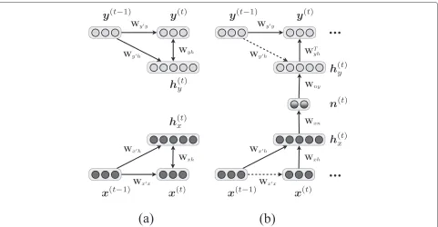
4 Related work
It is worth noting that we compare our method with the conventional method proposed by Wu et al. in [32], that also employed a CRBM for VC. Figure 2 shows the com-parison of graphical models among three methods. Wu’s method directly uses CRBM to estimate the target features y(t) from the inputx(t)along with the latent featuresh(t) to capture the linear and non-linear relationship between the source and the target features (Figure 2b). On the other hand, our method (Figure 2c) uses two CRBMs for each of the source and the target speakers to obtain their
latent featuresh(xt)andh(yt), capturing time-related infor-mation (fromt −1 to t frames). Connecting the latent features using a NN, the entire conversion network of our method consequently forms a deep architecture. Our pre-vious approach [25] has a deep network similar to that of the proposed method (Figure 2a); however, the differ-ence is that it involves time-related relationships in the network.
Since the acoustic signals we are targeting are time-series data, the model that captures time-related informa-tion will provide us with the better performance.
5 Experiments
5.1 Conditions
In our experiments, we conducted voice conversion using the ATR Japanese speech database [42], compar-ing our method (speaker-dependent restricted Boltzmann machines; say ‘SD-CRBM’) with four methods: the well-known GMM-based approach (‘GMM’), conventional NN-based voice conversion [18] (‘NN’), our previous work [25] (‘SD-RBM’) and, for a reference, a recurrent neu-ral network with randomly-initialized weights (‘RNN’). In order to evaluate our method under various circum-stances, we tested male-to-female (the source and the target speakers are identified with MMY and FTK in the database, respectively), female-to-female (FKN and FTK), and male-to-male (MMY and MHT) patterns.
For an input vector, we calculated 24-dimensional MFCC features from 513-dimensional STRAIGHT spec-tra [43] using the filter-theory [44] to decode the MFCC back to STRAIGHT spectra in the synthesis stage. Each speech signal was sampled at 12 kHz and windowed with a 25-ms Hamming window every 10 ms. Unlike our previ-ous work [25], we processed the obtained MFCC with zero component analysis (ZCA) whitening [38], where we con-firmed it worked better than without whitening, especially for ‘NN.’ The parallel data of the source/target speakers processed by dynamic programming were created from 216 word utterances in the dataset and were used for the training of each method (note that two CRBMs for ‘SD-CRBM’ and two RBMs for ‘SD-RBM’ can be trained without the necessity of using parallel data, although we used the same parallel training data for the CRBMs and the RBMs in this research.)
The network-based approaches (CRBM’, ‘SD-RBM’, ‘NN’, and ‘RNN’) were trained using gradient descent with a learning rate of 0.01 and momentum of 0.9, with the number of epochs being 400. The parame-ters of ‘NN’ and ‘RNN’ were initialized randomly. All the network-based methods had four layers including an input layer, two hidden layers, and an output layer. Other con-figurations, such as the number of hidden units, will be discussed in the following section.
4.80 4.93 5.05 5.18 5.30
24 48 72
MCD (dB)
Number of hidden units SD-CRBM SD-RBM
NN RNN
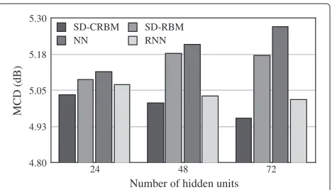
Figure 3Changing hidden units.The values show averaged
Mel-cepstral distortion with varying numbers of hidden unitsJfor all network-based methods (N=20, 000).
For the GMM-based approach, we used diagonal covari-ance matrices without global varicovari-ance and dynamic features.
For the objective test, 15 sentences (about 60 s long) that were not included in the training data were arbitrarily selected from the database (identified with SDA01∼SDA15). For the objective evaluation, we used Mel-cepstral distortion (MCD) to measure how close the converted vector is to the target vector in Mel-cepstral space. The MCD is defined as below:
MCD [dB]= 10 ln 10
' ( ( )224
d=1
cd−cd 2
(37)
wherecdandcddenote thedth original target MFCC and the converted MFCC, respectively. The smaller the value of MCD is, the closer the converted spectra are to the tar-get spectra. We calculated the MCD for each frame in the training data and averaged the MCD values for the final evaluation.
4.97 4.99 5.00 5.02 5.03
1 2 3 4 5
MCD (dB)
Number of previous frames
Figure 4Changing previous frames.The values show averaged
5.00 5.08 5.15 5.23 5.30
8 16 32 64 128
MCD (dB)
Number of mixtures
Figure 5Changing mixtures.The values show averaged
Mel-cepstral distortion with varying numbers of mixturesMfor GMM method (N=20, 000).
For the subjective evaluation, ABX listening tests were conducted, where nine participants listened to five pairs of converted speech signals (from a development set, which was used for the determination of model parameters) pro-duced using our approach (‘SD-CRBM’) and the converted speech signals produced by the other methods (‘SD-RBM’, ‘NN’, ‘RNN’, and ‘GMM’) along with an original target speech signal (generated from analysis-by-synthesis). We evaluated the models, which were trained using N = 5, 000 orN =20, 000 training frames. They then selected thebetterone in terms of speaker identity (how well they can recognize the speaker from the converted speech) and speech quality (how clear and natural the converted speech is).
5.2 Determining appropriate parameters
In this section, we report preliminary experiments in which we tested various models with different hyper
4.70 4.98 5.25 5.53 5.80
5k 10k 20k 40k
MCD (dB)
Number of training frames
SD-CRBM SD-RBM NN RNN GMM
Figure 6Male-to-female voice conversion results.The values show averaged Mel-cepstral distortion for each method with varying amounts of training data.
5.05 5.19 5.33 5.46 5.60
5k 10k 20k 40k
MCD (dB)
Number of training frames
SD-CRBM SD-RBM NN RNN GMM
Figure 7Female-to-female voice conversion results.The values show averaged Mel-cepstral distortion for each method with varying amounts of training data.
parameters to determine the appropriate ones. All models were trained usingN =20, 000 frames from the male-to-female training data and evaluated using a development set of five sentences (identified with SDA16∼SDA20 in the database) that were not included in either the training set or the test set.
5.2.1 Network-based methods
Here, we will see how our approach works as the number of hidden units J in each hidden layer changes, com-paring it to four network-based methods (‘SD-CRBM’, ‘SD-RBM’, ‘NN’, and ‘RNN’). In this preliminary experi-ment, three architectural patterns were tested, whereJ = 24, 48, and 72. We usedL = 0, which forms a four-layer network for all methods (for example, whenJ = 48 is
4.80 5.03 5.25 5.48 5.70
5k 10k 20k 40k
MCD (dB)
Number of training frames
SD-CRBM SD-RBM NN
RNN GMM
Preference score
0.00 0.25 0.50 0.75 1.00
SD-RBM NN RNN GMM
SD-CRBM Opponent
Figure 9Subjective preference scores w.r.t. speaker identity (in caseN=5, 000).Our method ‘SD-CRBM’ was compared to four other methods: ‘SD-RBM’, ‘NN’, ‘RNN’, and ‘GMM’.
used, the numbers of units in ‘NN’ from the input/source layer to the output/target layer become 24, 48, 48, and 24 in order). For ‘SD-CRBM’, we set P = 1 (1 delay for ‘RNN’ as well), which means we take into account only one previous frame.
Figure 3 compares the averaged MCD obtained for each architecture. As shown in Figure 3, our method ‘SD-CRBM’ performed the best of all the methods for each case. The interesting point is that the more hidden units the network has, the better performance it provides for ‘SD-CRBM’ and ‘RNN’, while it is the other way around for ‘SD-RBM’ and ‘NN’. This is considered to be due to over-fitting to the training data for ‘SD-RBM’ and ‘NN’ when the number of parameters is large (e.g., J = 72), while ‘SD-CRBM’ and ‘RNN’ still required parameters to fit the models that capture time-series data.
For the remaining experiments in this paper, the best architectures for each method were used, i.e.,J = 24 for ‘SD-RBM’ and ‘NN’, andJ=72 for ‘SD-CRBM’ and ‘RNN’.
Preference score
0.00 0.25 0.50 0.75 1.00
SD-RBM NN RNN GMM
SD-CRBM Opponent
Figure 10Subjective preference scores w.r.t. speech quality (in caseN=5, 000).Our method ‘SD-CRBM’ was compared to four other methods: ‘SD-RBM’, ‘NN’, ‘RNN’, and ‘GMM’.
0 0.25 0.50 0.75 1.00
SD-RBM NN RNN GMM
Preference score
SD-CRBM Opponent
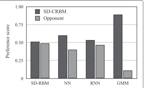
Figure 11Subjective preference scores w.r.t. speaker identity (in caseN=20, 000).Our method ‘SD-CRBM’ was compared to four other methods: ‘SD-RBM’, ‘NN’, ‘RNN’, and ‘GMM’.
5.2.2 The number of previous frames
We further investigated the performance of our method ‘SD-CRBM’ with the hidden units of J = 72, chang-ing the number of previous frames in the CRBM as P = 1, 2, 3, 4, 5. The evaluation results are described in Figure 4, showing the averaged MCDs obtained from each case. As shown in Figure 4, we could not necessarily obtained a better performance as the number of previous frames increased. One reason is that the neighbor source vectors previous to the current one contained similar information, and only a few source vectors were required to estimate the current target vector. Therefore, the poor performance with the larger number of previous frames (e.g.,P = 4) was caused because the parameter estima-tion became more difficult as the redundant parameters increased.
In the remaining experiments, we used P = 1, which provided the best performance in the preliminary experiment.
0 0.25 0.50 0.75 1.00
SD-RBM NN RNN GMM
Preference score
SD-CRBM Opponent
Table 1pvalues between our method and each method
w.r.t. speaker identity in caseN=5, 000
SD-RBM NN RNN GMM
p 0.2796 0.1636 0.0013 0.0032
The values that satisfyp<0.1are in italics.
5.2.3 GMM-based method
For the GMM-based voice conversion (‘GMM’), we tried and evaluated five mixtures (8, 16, 32, 64, and 128 mix-tures) to determine an appropriate number of mixtures. Figure 5 shows the averaged MCDs over the develop-ment set when using the GMM with various mixtures. As shown in the figure, the GMM with 64 mixtures per-formed the best of all. Therefore, we used mixtures of 64 for ‘GMM’ in the evaluation experiments described in Section 5.3.
5.3 Evaluation
In this section, we evaluate our method (‘SD-CRBM’) comparing it with four methods (‘SD-RBM’, ‘NN’, ‘RNN’, and ‘GMM’) using objective and subjective criteria for each pair of speakers, by changing the number of training frames asN=5, 000, 10,000, 20,000, and 40,000.
5.3.1 Results
Figures 6, 7, and 8 summarize the experimental results for the test data, comparing each method with respect to objective criteria for male-to-female, female-to-female, and male-to-male voice conversion, respectively. As shown in these Figures, the MCDs decreased as the num-ber of training data increased in most cases (regardless of the gender or the method). Furthermore, our approach outperformed the other methods in every case, except for the case where N = 20, 000 in the male-to-male experiment.
Figures 9 and 10 show the results of subjective evalua-tion comparing each method in terms of speaker identity and speaker quality, respectively, when we use training samples ofN = 5, 000. Figures 11 and 12 also show the subjective evaluation results when we use training sam-ples ofN = 20, 000. We also list thepvalues produced by pairwiset-testing for each experiment in Tables 1 and 2, and in Tables 3 and 4, in terms of speaker identity and speech quality, respectively. As shown in Figures 11 and 12, our method performed better than each oppo-nent method in regard to mean preference score in
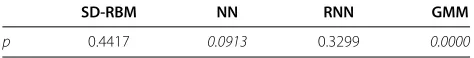
Table 2pvalues between our method and each method
w.r.t. speaker identity in caseN=20, 000
SD-RBM NN RNN GMM
p 0.0913 0.4417 0.0913 0.0001
The values that satisfyp<0.1are in italics.
Table 3pvalues between our method and each method
w.r.t. speaker quality in caseN=5, 000
SD-RBM NN RNN GMM
p 0.2796 0.4343 0.3096 0.0032
The values that satisfyp<0.1are in italics.
terms of both speaker identity and speech quality. How-ever, as shown in Tables 1, 2, 3, and 4, we could not, unfortunately, obtain a significant difference between our method and the other methods in some cases (e.g., ‘NN’ with respect to (w.r.t.) speaker identity, and ‘SD-RBM’ and ‘RNN’ w.r.t. speech quality whenN = 20, 000 training frames were used). We obtained significant differences at a significance level of 0.1 in the other cases.
5.3.2 Discussion
In objective criteria, our approach (‘SD-CRBM’) outper-formed the other methods, including the popular GMM-based voice conversion method, in most cases. In sub-jective criteria as well, we obtained significantly better performance compared with each opponent, in terms of speaker identity and/or speech quality (to be specific, in terms of both speaker identity and speech quality for ‘GMM’, in terms of only speech quality for ‘NN’, in terms of only speaker identity for ‘SD-RBM’ and ‘RNN’). The reason for the improvement is attributed to the fact that our time-involving, high-order conversion sys-tem using CRBMs is able to capture and convert the abstractions of speaker individualities better than the other methods. In particular, as shown in Figures 6, 7, and 8, our approach achieved high performance in MCD criteria. This is because the CRBMs captured time-series data more appropriately and alleviated estimation errors.
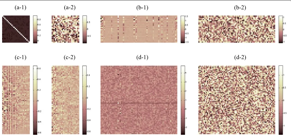
One interesting point is that ‘NN’ and ‘RNN’, which were based on random initialization in weight parame-ters, produced unstable performance (e.g., the MCD by ‘NN’ increased even as the number of training frames increased from 10,000 to 20,000 in male-to-female con-version, and the MCD by ‘RNN’ also increased as the number of training data changed from 20,000 to 40,000 in male-to-male conversion). This is caused by a fall into local minima starting from the randomly-initialized weights. Figure 13 shows some of the converged weights in the network, comparing ‘RNN’ and ‘SD-CRBM’, where
Table 4pvalues between our method and each method
w.r.t. speech quality in caseN=20, 000
SD-RBM NN RNN GMM
p 0.4417 0.0913 0.3299 0.0000
(a-1) (a-2) (b-1) (b-2)
(d-1) (c-2)
(c-1) (d-2)
Figure 13Estimated weights of the pre-trained RNN (·-1) and the randomly-initialized RNN (·-2).After 400 epochs (N=40, 000,J=72, male-to-female). (a) The weights from the previous target vector to the current target vectorWyy, (b) the weights from the second hidden layer to the current target vectorWyh, (c) the weights from the current source vector to the first hidden layerWxh, and (d) the weights from the first hidden layer to the second hidden layerW0.
the weights were pre-trained using speaker-dependent CRBMs and a concatenating NN followed by fine-tuning using RNN. As shown in Figure 13, the weights in ‘RNN’ were almost meaningless and messy; meanwhile, we see that the weights in ‘SD-CRBM’ had a sparse structure and operative bases. In general, an acoustic feature vec-tor at the last previous frame (v(t−1)) is very similar to the feature vector at the current frame (v(t)), and, therefore, we expect that the conversion matrix fromv(t−1) to v(t) may be close to an identity matrix. The recurrent weight obtained by our approach shown in Figure 13a-1 indicates this fact.
6 Conclusion
We presented a voice conversion method that combines dependent CRBMs and a NN to extract speaker-individual information for speech conversion. Through experiments, we confirmed that our approach is effective, especially in terms of MCD, compared with the well-known conventional GMM-based approach, a NN-based approach, and our own previous work, SD-RBM, (and recurrent neural network for a reference), regardless of the gender in conversion.
We also conducted ABX experiments for subjective evaluation. The results showed that the performance of our method was not always significantly different in comparison to NN, RNN, and SD-RBM; however, it did perform significantly better than these methods in terms of either speaker identity or speech quality. In
the future, we will work to improve our method so that it obtains better results in regard to the sense of hearing.
Competing interests
The authors declare that they have no competing interests.
Author details
1Graduate School of System Informatics, Kobe University, 1-1 Rokkodai, Nada-ku, 657-8501 Kobe Japan.2Organization of Advanced Science and Technology, Kobe University, 1-1 Rokkodai, Nada-ku, 657-8501 Kobe, Japan.
Received: 28 February 2014 Accepted: 11 December 2014
References
1. A Kain, MW Macon, inProceedings of IEEE International Conference on Acoustics, Speech and Signal Processing (ICASSP). Spectral voice conversion for text-to-speech synthesis, (1998), pp. 285–288
2. C Veaux, X Robet, inProceedings of Interspeech. Intonation conversion from neutral to expressive speech, (2011), pp. 2765–2768
3. K Nakamura, T Toda, H Saruwatari, K Shikano, Speaking-aid systems using GMM-based voice conversion for electrolaryngeal speech. Speech Commun.54(1), 134–146 (2012)
4. L Deng, A Acero, L Jiang, J Droppo, X Huang, inProceedings of IEEE International Conference on Acoustics, Speech, and Signal Processing (ICASSP). High-performance robust speech recognition using stereo training data, (2001), pp. 301–304
5. A Kunikoshi, Y Qiao, N Minematsu, K Hirose, inProceedings of Interspeech. Speech generation from hand gestures based on space mapping, (2009), pp. 308–311
6. R Gray, Vector quantization. ASSP Mag. IEEE.1(2), 4–29 (1984) 7. H Valbret, E Moulines, J-P Tubach, Voice transformation using PSOLA
technique. Speech Commun.11(2), 175–187 (1992)
9. T Toda, AW Black, K Tokuda, Voice conversion based on
maximum-likelihood estimation of spectral parameter trajectory. IEEE Trans. Audio Speech Lang. Process.15(8), 2222–2235 (2007) 10. E Helander, T Virtanen, J Nurminen, Gabbouj, Voice conversion using
partial least squares regression. IEEE Trans. Audio Speech Lang. Process.
18(5), 912–921 (2010)
11. C-H Lee, C-H Wu, inProceedings of Interspeech. Map-based adaptation for speech conversion using adaptation data selection and non-parallel training, (2006), pp. 2254–2257
12. T Toda, Y Ohtani, K Shikano, inProceedings of Interspeech. Eigenvoice conversion based on gaussian mixture model, (2006), pp. 2446–2449 13. D Saito, Yamamoto K, N Minematsu, K Hirose, inProceedings of
Interspeech. One-to-many voice conversion based on tensor representation of speaker space, (2011), pp. 653–656
14. D Saito, S Watanabe, A Nakamura, N Minematsu, inProceedings of Interspeech. Probabilistic integration of joint density model and speaker model for voice conversion, (2010), pp. 1728–1731
15. Z Jian, Z Yang, inProceedings of International Conference on Software Engineering, Artificial Intelligence, Networking, and Parallel/Distributed Computing. Voice conversion using canonical correlation analysis based on Gaussian mixture model, (2007), pp. 210–215
16. R Takashima, T Takiguchi, Y Ariki, inIEEE Spoken Language Technology Workshop (SLT). Exemplar-based voice conversion in noisy environment, (2012), pp. 313–317
17. M Narendranath, HA Murthy, S Rajendran, B Yegnanarayana, Transformation of formants for voice conversion using artificial neural networks. Speech Commun.16(2), 207–216 (1995)
18. S Desai, EV Raghavendra, B Yegnanarayana, AW Black, K Prahallad, in Proceedings of IEEE International Conference on Acoustics, Speech and Signal Processing (ICASSP). Voice conversion using artificial neural networks, (2009), pp. 3893–3896
19. Y-J Wu, H Kawai, J Ni, R-H Wang, inProceedings of IEEE International Conference on Acoustics, Speech, and Signal Processing (ICASSP). Minimum segmentation error based discriminative training for speech synthesis application, (2004), p. 629
20. E McDermott, TJ Hazen, J Le Roux, A Nakamura, S Katagiri, Discriminative training for large-vocabulary speech recognition using minimum classification error. IEEE Trans. Audio Speech Lang. Process.15(1), 203–223 (2007)
21. T Tomoki, K Tokuda, A speech parameter generation algorithm considering global variance for HMM-based speech synthesis. IEICE Trans. Inform. Syst.90(5), 816–824 (2007)
22. Z-H Ling, L-R Dai, Minimum Kullback-Leibler divergence parameter generation for HMM-based speech synthesis. IEEE Trans. Audio Speech Lang. Process.20(5), 1492–1502 (2012)
23. Z-H Ling, Y-J Wu, Y-P Wang, L Qin, R-H Wang, inBlizzard Challenge Workshop. USTC system for blizzard challenge 2006 an improved HMM-based speech synthesis method, (2006)
24. Z Wu, T Virtanen, T Kinnunen, ES Chng, H Li, inProceedings of the 8th ISCA Speech Synthesis Workshop. Exemplar-based voice conversion using non-negative spectrogram deconvolution, (2013), pp. 221–226 25. T Nakashika, R Takashima, T Takiguchi, Y Ariki, inProceedings of Interspeech.
Voice conversion in high-order eigen space using deep belief nets, (2013), pp. 369–372
26. P Smolensky, Information processing in dynamical systems: foundations of harmony theory. Parallel Distributed Process.1, 194–281 (1986) 27. GE Hinton, S Osindero, Y-W Teh, A fast learning algorithm for deep belief
nets. Neural Comput.18(7), 1527–1554 (2006)
28. Z-H Ling, L Deng, D Yu, Modeling spectral envelopes using restricted Boltzmann machines and deep belief networks for statistical parametric speech synthesis. IEEE Trans. Audio Speech Lang. Process.21(10), 2129–2139 (2013)
29. A-R Mohamed, GE Dahl, G Hinton, Acoustic modeling using deep belief networks. Audio Speech Lang. Process. IEEE Trans.20(1), 14–22 (2012) 30. V Nair, G Hinton, 3-D object recognition with deep belief nets. Adv.
Neural Inform. Process. Syst.22, 1339–1347 (2009)
31. T Deselaers, S Hasan, O Bender, H Ney, inProceedings of the Fourth Workshop on Statistical Machine Translation. A deep learning approach to machine transliteration, (2009), pp. 233–241
32. Z Wu, ES Chng, H Li, inProceedings of the IEEE China Summit and International Conference on Signal and Information Processing (ChinaSIP). Conditional restricted Boltzmann machine for voice conversion, (2013) 33. C Ling-Hui, L Zhen-Hua, S Yan, D Li-Rong, inProceedings of Interspeech.
Joint spectral distribution modeling using restricted Boltzmann machines for voice conversion, (2013), pp. 3052–3056
34. DH Ackley, GE Hinton, TJ Sejnowski, A learning algorithm for Boltzmann machines. Cogn. Sci.9(1), 147–169 (1985)
35. Y Freund, D Haussler, Unsupervised learning of distributions of binary vectors using two layer networks. Adv, Neural Inform. Process. Syst.4, 912–919 (1991)
36. GE Hinton, RR Salakhutdinov, Reducing the dimensionality of data with neural networks. Science.313(5786), 504–507 (2006)
37. G Hinton, inTech. Rep. Department of Computer Science. A practical guide to training restricted Boltzmann machines (University of Toronto, 2010) 38. A Krizhevsky, G Hinton,Learning multiple layers of features from tiny images.
(Computer Science Department, University of Toronto, Tech. Rep, 2009) 39. K Cho, A Ilin, T Raiko, inArtificial Neural Networks and Machine
Learning–ICANN 2011. Improved learning of gaussian-bernoulli restricted Boltzmann machines, (2011), pp. 10–17
40. GW Taylor, GE Hinton, ST Roweis, inAdvances in Neural Information Processing Systems. Modeling human motion using binary latent variables, (2006), pp. 1345–1352
41. R Pascanu, T Mikolov, Y Bengio, On the difficulty of training recurrent neural networks. (2012)
42. A Kurematsu, K Takeda, Y Sagisaka, S Katagiri, H Kuwabara, K Shikano, ATR japanese speech database as a tool of speech recognition and synthesis. Speech Communication.9(4), 357–363 (1990)
43. H Kawahara, M Morise, T Takahashi, R Nisimura, T Irino, H Banno, in Proceedings of IEEE International Conference on Acoustics, Speech and Signal Processing (ICASSP). Tandem-straight: a temporally stable power spectral representation for periodic signals and applications to interference-free spectrum, f0, and aperiodicity estimation, (2008), pp. 3933–3936 44. B Milner, X Shao, inProceedings of Interspeech. Speech reconstruction
from mel-frequency cepstral coefficients using a source-filter model, (2002), pp. 2421–2424
Submit your manuscript to a
journal and benefi t from:
7Convenient online submission 7Rigorous peer review
7Immediate publication on acceptance 7Open access: articles freely available online 7High visibility within the fi eld
7Retaining the copyright to your article
![Figure 2 Model structures of the related systems. (a) Our earlier work, speaker-dependent RBM, (b) CRBM proposed in [32], and (c) ourproposed method, speaker-dependent CRBM.](https://thumb-us.123doks.com/thumbv2/123dok_us/9591233.1941680/6.595.57.541.491.703/figure-structures-earlier-speaker-dependent-proposed-ourproposed-dependent.webp)