Computational Intelligence and Complexity Measures for Chaotic Information Processing

(1)

University of New Orleans University of New Orleans

ScholarWorks@UNO

University of New Orleans Theses and

Dissertations Dissertations and Theses 5-16-2008

Computational Intelligence and Complexity Measures for Chaotic

Information Processing

Davoud Arasteh

University of New Orleans

Follow this and additional works at: https://scholarworks.uno.edu/td

Recommended Citation Recommended Citation

Arasteh, Davoud, "Computational Intelligence and Complexity Measures for Chaotic Information Processing" (2008). University of New Orleans Theses and Dissertations. 834.

https://scholarworks.uno.edu/td/834

(2)

COMPUTATIONAL INTELLIGENCE AND COMPLEXITY MEASURES

FOR CHAOTIC INFORMATION PROCESSING

A Dissertation

Submitted to the Graduate Faculty of the University of New Orleans

in partial fulfillment of the requirements for the degree of

Doctor of Philosophy in

Engineering and Applied Science

by

Davoud Arasteh

B.S. (National University of Iran, Tehran) 1991 M.S. (Amir Kabir University of Technology, Tehran) 1994

M.S. (University of Louisiana, Lafayette) 2002

(3)

(4)

DEDICATION

To my wife, Mehrdokht my daughters, Ailar and Aileen

my son, Aidin

(5)

ACKNOWLEDGEMENTS

I am deeply indebted to my advisors Dr. George Ioup and Dr. Juliette Ioup for their continuous support and encouragement throughout my doctoral studies. Their patience, enthusiasm, and generous contribution of time and resources have greatly helped me to achieve my goals and kept this research progressing with good insight and advice. I am especially thankful for their trust in my ideas and abilities and for the opportunities they have offered me. I would like to thank the committee co-chair Dr. Abolfazl Amini for all the knowledge and support. He served on both my general examination and dissertation committees, encouraging me every step of the way. I am fortunate to have had the guidance and support of many faculties at UNO, especially Dr. Jinke Tang and Dr. Dimitrios Charalampidis. They generously served on both general examination and dissertation committees.

I would like to thank the department staff especially Sandra Merz and Zella Huaracha. They are both very knowledgeable and genuinely friendly. They took care of every administrative bump I ran into.

Finally, I wish to thank and express my appreciation to my family for their immeasurable emotional support and encouragement, which was indispensable during my time in graduate school. Thank you for keeping the faith and getting me here.

During the years the material in this dissertation has been presented at conferences and parts have also been accepted for publication. Here are some of the places where it occurs in proceedings and journals.

 Algorithmic Complexity Measure and Lyapunov Matrices of the Dynamical Systems,

Paper Number: ENT 108-099, 2006 IJME/Intertech International Conference Proceedings.

 Algorithmic Complexity Measure of the Dynamical Systems, Intelligent Engineering Systems through Artificial Neural Networks, Volume 16, pp. 161-167, ASME Press 2006.

 Ultra High-Speed Microbridge Chaos Domain, Intelligent Engineering Systems through Artificial Neural Networks, Volume 17, pp. 365-370, ASME Press 2007.

 Computing Algorithmic Complexity Using Advance Sampling Technique, Intelligent Engineering Systems through Artificial Neural Networks, to appear in Volume 18, ASME Press 2008.

 Algorithmic Complexity Analysis of Best ½-Rate Convolutional Codes with Chaotic-Encrypted Data,Intelligent Engineering Systems through Artificial Neural Networks, to appear in Volume 18, ASME Press 2008.

 Measures of Order in Dynamic Systems, Paper Number: CND-06-1119, Journal of Computational and Nonlinear Dynamics, to appear in Volume 3, July 2008.

(6)

LIST OF FIGURES

1.1 A heated fluid layer (Bernard experiment) ...9

1.2 Bifurcation diagram,Xnvs.μfor logistic mapXn+1=μXn(1−Xn) ...15

2.1 Exponential divergence of two nearby trajectories for a dynamical flowX(t)X(0)et with future prediction time _        _ ) 0 ( ) ( ln 1 X t X t_p      ...19

2.2 (a) Logistic bifurcation map including transient solutions (b) Logistic bifurcation map without transients solutions (c) Lyapunov exponentλvs....24

2.3 Divergence of trajectories from a small sphere of initial conditions ...33

2.4 Tangent space trajectories...36

2.5 (a) Divergence of trajectories (b) reorthonormalization at time incrementτ...36

2.6 Henon map attractors density distribution for different values of the control parametera and b=0.3. 1-Cycle at a=0, 1→2 Cycle at a=0.36, 2-Cycle at a=0.5, 2→4 Cycle at a=0.913, 4-Cycle ata=1, 4→8 Cycle at a=1.026...51

2.7 Henon map attractors density distribution for different values of the control parametera andb=0.3. 8→16 Cycle at a= 1.0511, 16→32 Cycle at a= 1.0565, chaotic state ata= 1.1, Chaos→7 Cycle at a=1.2266, 7 Cycle ata= 1.227, other 7-cycle ata= 1.3. ...52

2.8 Henon map attractors density distribution for different values of the control parametera andb=0.3. Chaotic states at a=1.35, 1.39 and 1.4. ...53

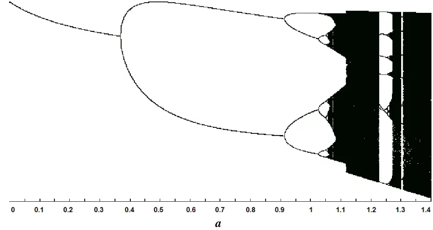
2.9 Henon map bifurcation diagram vs. control parameterawhenb=0.3 ...53

2.10 Henon map bifurcation diagram vs. control parameterawhenb=0.3 ...54

2.11 Henon map Largest Lyapunov exponent vs.a, b= 0.3 ...55

3.1 Some types of Josephson junctions. (a) Thin-film tunnel junction. (b) Point contact. (c) Thin-film weak link ...62

3.2 DC current-voltage characteristics for a weak and tunnel junction...63

3.3 Stewart-McCumber model: Resistively and capacitively shunted junction (RCSJ) model of a Josephson junction. The cross represents the coherent Cooper pair tunneling channel ...65

3.4 Josephson Junction I-V characteristic curves; (a) hysteretic (b) non-hysteretic...68

(10)

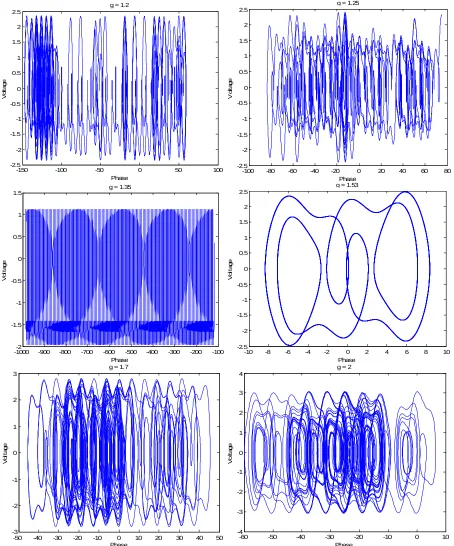
3.6 Josephson junction system phase portraits for different applied driving amplitudes (g).

With dissipation coefficientk=0.5 and driving frequency ωd=2/3, over 1.5×104iterations,

after 2×103transient solutions ...71

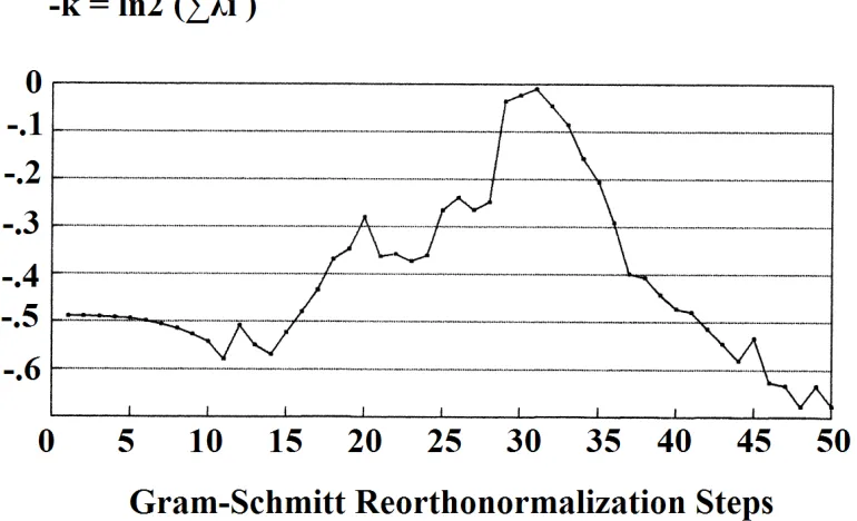
3.7 Josephson junction system LE sum (ln2)∑λiplotted vs. GSR steps. Control parameters:g

= 3.8,k=0.5,ωd=2/3 over iterations 2×105...75

3.8 Josephson junction system maximum LE vs. number of iterations. Control parameters:g

= 3.8,k=0.5,ωd=2/3 and GSR step = 5 ...75

3.9 Josephson junction bifurcation diagram for microwave radiation amplitude g [∆g =

0.001],k=0.5,ωd=2/3...76

3.10 Josephson junction system first LE calculated by (a) GSR method (b) NRNO method.

Control parameters: 0.9≤g≤1.5 [∆g= 0.001],k=0.5,ωd=2/3 ...77

3.11 Josephson junction system LE spectrum (λ1, λ2, λ3 and ∑λi) by GSR method. Control

parameters: 0.9 ≤g ≤1.5 [∆g = 0.001], k=0.5, ωd=2/3 over 105 iterations after 2×104

transients ...79

3.12 Josephson junction system LE spectrum(λ1, λ2,∑λi, and.F) by NRNO method. Control

parameters: 0.9 ≤g ≤1.5 [∆g = 0.001], k=0.5, ωd=2/3 over 105 iterations after 2×104

transients ...80

3.13 Josephson junction system LE spectrum (λ1,λ2,∑λi, and .F) by NRNO method, control

parameters: microwave amplitude 0.9 ≤g ≤1.5 [∆g = 0.001], k=0.5, ωd=2/3 over 105

iterations after 2×104transients ...81

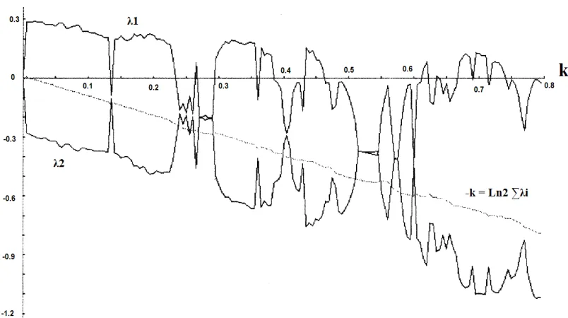
3.14 Josephson junction system LE spectrum (λ1, λ2, λ3) and (ln2)∑λi) vs. dissipation

coefficient 0≤k≤0.8 [∆k= 0.01], microwave amplitude and frequency g= 3.8,ωd= 0.5,

over 5×104iterations ...82

3.15 Portrait of Josephson electrical voltage vs. phase. Periodic oscillations at k = 0.25, 0.4,

0.5, 0.6, 0.8, 3.5 and 5. Chaotic oscillations corresponding tok= 0.05, 0.2, 0.3, 0.7, and

2.9. Microwave amplitude and frequency:g= 3.8,ωd= 0.5 ...82

3.16 (a) First LE (λ1) and (b) Josephson junction positive first LE (λ1+) forgvs.k.

0.9≤g≤1.5, [Δg=0.01]; k: 0≤k≤0.9, [Δk=0.01];ωd=2/3, 105iterations, 104transients,

ε= 0.01, GSR steps = 5...86

3.17 (a) Josephson junction system first LE (λ1), (b) positive first LE (λ1+) for g vs. ωd.

0.9≤g ≤1.5, Δg=0.01; 0≤ωd≤0.9 [Δωd= 0.01],k = 0.5, 105 iterations, 104transients,

ε= 0.01, GSR steps= 5...87

3.18 (a) Josephson junction system first LE (λ1), (b) positive first LE (λ1+) forkvs. ωd.

0≤k≤1 [Δk= 0.01]; 0≤ωd≤1 [Δωd=0.01];g=3.8, 105iterations, 104transients,

(11)

3.19 Josephson junction system strange attractor forg= 1.16,k= 0.5,ωd= 2/3...91

3.20 Josephson junction system Kaplan-York fractal dimension and LE spectrum (λ1, λ2, λ3). 0.9≤g≤1.5 [Δg = 0.01],k= 0.5, ωd= 2/3, 105iterations, 104transients,ε= 0.01, GSR step 5.. ...92

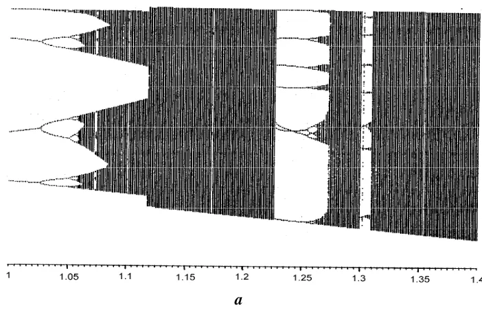
3.21 Henon map (a) bifurcation diagram (b) K-S entropy for 1≤a ≤1.4 with increment 0.01 ...94

4.1 LZ complexity analysis flowchart for sequenceSof lengthN...110

4.2 (a) Logistic map bifurcation (b) LZC when 3≤μ≤4 ...112

4.3 Henon map phase space



X_n,Y_n



forb=0.3,a= 1.4...114

4.4 LZ complexity of strings constructed from the Henon map b = 0.3, 1 ≤a ≤1.4 [Δa=0.001] ...115

4.5 Henon map bifurcation diagramb= 0.3...115

4.6 Josephson junction system strange attractor and its Poincare sectiong= 1.2,k= 0.5, ω_d= 2/3 ...117

4.7 Josephson junction system strange attractor probability density functiong= 1.2, k= 0.5, ω_d= 2/3 ...117

4.8 Josephson junction system LZ complexity vs. microwave amplitudeg,[Δg= 0.001]; k=0.5,ωd=2/3 ...118

4.9 Josephson junction system bifurcation diagram vs. microwave amplitudeg,[Δg= 0.001] k=0.5,ωd= 2/3 ...118

4.10 Josephson junction system (a) bifurcation diagram, (b) first LE (c) LZC vs. microwave frequency ωd. Microwave amplitude and system dissipation coefficient are 3.8 and 0.5 respectively ...119

4.11 One branch of the unstable manifold for (a)ρ<ρh (b) ρ>ρh and (c)ρ=ρh ...125

4.12 Variation of the angle with the Lorenz system x-axis in 0≤ρ≤100 range ...126

4.13 Lorenz attractor forσ= 10,β= 8/3 andρ= 28...127

4.14 Lorenz attractor projection forσ= 10, β= 8/3 andρ= 28 on (a)z-yplane (b)y-xplane (c) z-xplane ...127

4.15 Comparision of Lorenz system LEs sum and flow divergence vs. GSR integration number for fixed parameters value,σ=10,β=8/3,ρ=25 ...130

4.16 Comparision of Lorenz system LEs sum and flow divergence vs. GSR integration number and dynamic system integration time step.σ=10,β=8/3,ρ=25 ...130

(12)

4.18 Lorenz system LZC. Control parameters: 0≤ρ ≤ 500, Δρ=0.1,σ= 10,β= 8/3 ...133

4.19 Lorenz system largest LE. Control parameters: 0≤ρ ≤ 500, Δρ=0.1,σ= 10,β= 8/3 ....134

4.20 Lorenz bifurcation diagram. (a) without window (b) with window size = 5. Control

parameters: 0 ≤ρ ≤ 500 [Δρ=0.1]; σ= 10,β= 8/3, N = 1600, transient states = 4000;

tolerance=0.01, integration time step= 0.01 ...135

5.1 Equivalent circuit configuration of the Josephson Tetrode Microbridge device ...138

5.2 Waveforms of the tetrode microbridge electrical voltages at variousRn14quasi-periodic

oscillations at Rn14 = 0, Rn14 = 0.19, Rn14 = 0.4, Rn14 = 1.5, Rn14 = 2.2 and Rn14 = 2.8.

Chaotic oscillations phase portraits corresponding toRn14 = 0.7, Rn14 =1.25, Rn14= 1.4,

and periodic oscillations atRn14=3 ...143

5.3 Tetrode microbridge electrical voltages phase portrait. Quasi-periodic oscillations atRn14

= 0, 0.19, 0.4, 1.5, 2.2 and 2.7. Chaotic oscillations phase portraits corresponding toRn14

= 0.7, 1.25, 1.39 and periodic oscillationRn14= 3 ...146

5.4 Tetrode microbridge LE vs. normal resistance Rn14 when varied from 0 to 3 with step

0.01...151

5.5 Tetrode microbridge bifurcation diagram for voltage V12 vs. Rn14 with integration time

step, 0.01, transients discarded, 3000, integration numbers, 4000, tolerance, 0.0005,

Tp=2π...151

5.6 Tetrode microbridge LZC plot for voltageV23andV14vs.Rn14...152

5.7 Tetrode microbridge electrical voltages frequencies as function ofRn14...154

5.8 Tetrode microbridge under microwave excitation Lyapunov exponent. 0≤g≤1,

Δg= 0.01,ωd= 1,Rn14= 1.4Ω...157

5.9 Tetrode microbridge under microwave excitation. Electrical voltages phase portrait and

temporal waveforms at various microwave amplitude 0≤g≤1. Microwave frequencyωd

= 1 andRn14= 1.4Ω. Chaotic oscillations correspond to 0≤g< 0.12, 0.2≤g≤0.4 andg

= 0.7. Otherwise the states are quasi-periodic oscillations ...157

5.10 Tetrode microbridge under microwave excitation. (a) first LE λ1 (b) positive first

Lyapunov exponentλ1+. Control parameters: drive amplitude 0≤g≤1 [Δg = 0.01], and 0

≤Rn14 ≤3 [ΔRn14 =0.01], driving frequency is ωd = 1. First LE maximum value is 0.16

and occurs wheng= 0.97,Rn14= 2.15 ...165

5.11 Tetrode microbridge under microwave excitation. (a) first LEλ1 (b) positive maximum

LEλ+. Control parameters: driving amplitude 0≤g≤1 [Δg = 0.01], driving frequency 0

≤ωd≤7 [Δωd =π/100], andRn14= 1.4. Maximum positive first LE,λ1+= 0.398 occurs at

(13)

5.12 Tetrode microbridge under microwave excitation phase portrait. The maximum positive

first Lyapunov exponent (λ1+= 0.3983) atg= 0.96 and ωd=0.2513...168

5.13 Tetrode microbridge under microwave excitation. Voltages phase portraits and temporal

waveforms. Control parameters:ωd=π/10,Rn14= 0. Showing two quasiperiodic states at

g= 0.1, 0.2, and a chaotic state at 0.3 ...168

5.14 Tetrode microbridge under microwave excitation phase portraits and temporal voltages

waveform. Control parameters for microwave amplitude and frequency areg= 0.1,

ωd=π/10.Rn14values are 0.4, 0.5, 0.7...170

6.1 LE spectrum for feedback controlled system whenB= 3,C= 20, 30≤A≤31

[ΔA= 0.01] and −1.5≤D≤1.5 [ΔD= 0.01] ...174

6.2 First and second Lyapunov exponent plots for 4-dim feedback-controlled system ...175

6.3 Chaos and hyperchaos regions for 4-Dim feedback-controlled system defined by (Eqs.

6.3) (a) Chaos and hyperchaos region. (b) Hyperchaos region...176

6.4 Kaplan-York fractal dimension vs. parametersDandA...177

6.5 Lyapunov exponentsλ1, λ2forD: −1.5≤D≤1.5 [ΔD= 0.01],A=36,B=3 andC=20 over

105iterations with 2x104transients,ε=0.001, GSR step 1 ...178

6.6 Lempel-Ziv complexity for a feedback-controlled system when A=36,B= 3,C = 20, 30

≤D≤39, ΔD= 0.01,n= 16300,ε= 0.001 (a) τ= 100 with maximum LZC=974 (b) when

τ= 50 with maximum LZC =761...181

6.7 Feedback-controlled system phase portraits and time series diagram (a) hyperchaotic

state,D=0.75 (b) Chaotic state,D=−1.5 (c) Periodic state,D=−0.75...182

6.8 Lyapunov exponentsλ1, λ2, λ3 for 8-dim feedback-controlled system for−1.5≤D≤1.5,

A=30, B=3, C=20, over 105 iterations with 104transients removal, integration time-step

0.01, GSR step 1 ...186

6.9 8-dim feedback-controlled system phase portraits. Hyperchaotic state,D=1, 1.25 periodic

states,D=−0.75,−0.22, −2.5; and an example of chaotic state atD=−1.25; A=30, B=3,

C=20...187

6.10 Lempel-Ziv complexity for 8-dim feedback-controlled system when A=30, B=3, C=20,

D: −1.5 ≤D ≤1.5 [ΔD=0.01], buffer size 16300, integration step-size 0.001 over 105,

after 104transients removed, advance time-stepτ=10...188

6.11 Din system Lyapunov exponentsλ1, λ2forD:−20≤D≤−2, [ΔD=0.1],A=16,B=3,C=10,

105iterations, 104transients, ε=0.01, GSR step 1. ...189

6.12 Din system phase portraits. Chaotic states occur atD=−20,−6 and periodic states atD=

−13 and−2.5. ...190

6.13 Din system typical chaotic state phase portraits inxi-xjplane whenD=−47.4.A=16,B=3,

C=10...191

(14)

ΔD = 0.1, buffer size 16300, integration step-size 0.001 over 105, 104 transients,

advance sampling stepτ=100 ...192

7.1 Duffing system resonance curveA(Ω) ...196

7.2 Duffing system bifurcation diagram 0.35≤F≤0.663 [ΔF= 0.001],Ω=1,μ=0.5...197

7.3 Duffing system LZC plot for 0.35≤F≤0.663 [ΔF= 0.001],Ω=1,μ=0.5...197

7.4 Duffing system topological entropy plot for 0.35 ≤F ≤0.663 [ΔF=0.001], Ω=1, and μ=0.5,n=3x105, tolerance=0.005...198

7.5 Addition rule verification. 0 ≤M ≤1 [ΔM= 0.01], 0 ≤A ≤1, [ΔA=0.01], K=0.5, 2×105 iterations, time-step 0.1, 104transients, GSR step 1 ...200

7.6 (a) First Lyapunov exponent (b) Positive first LE. 0 ≤M ≤1, [ΔM=0.01], 0 ≤A ≤1, [ΔA=0.01], K=0.5, over 2x105 iterations, integration time-step 0.1, after 104 transients, GSR step 1 ...201

7.7 (a) Second Lyapunov exponent (b) Positive second LE, hyperchaos regions. 0 ≤M ≤1, [ΔM=0.01], 0≤A≤1, [ΔA=0.01],K=0.5, over 2×105iterations, integration time-step 0.1, transients 104...204

7.8 Hyperchaotic attractor atK= 0.5,M= 0.29,A= 0.22. λ1= 0.21, λ2= 0.014 ...205

7.9 (a) Third LE (b) Fourth LE. Control parameters: 0 ≤M ≤1, [ΔM=0.01], 0 ≤A ≤1, [ΔA=0.01],K=0.5, 2×105iterations, integration time-step 0.1, after 104transients ...206

7.10 Kaplan-York fractal dimension. Control parameters: 0 ≤M ≤1, [ΔM=0.01], 0 ≤A≤1, [ΔA=0.01], K=0.5, over 2×105 iterations with integration time-step 0.1 and after 104 transients ...207

7.11 Bifurcation diagram for maximum amplitudeX2vs. the coupling constant K[ΔK=0.0002] (a) Tp=2π(b) Tp=10 (c) Bifurcation diagram for maximum velocity amplitude Y2. Same dynamical states occur for the same values of the coupling constantK.M= 0.8, A= 0.5, integration time-step 0.1 over 5×104iterations after 500 transients, tolerance ~ 0.001 ..209

7.12 Lyapunov exponent spectrum in terms of coupling constantK[ΔK=0.01]. M=0.8, A=0.5, integration time-step 0.1 over 2x105iterations after 104transients, GSR step 1 ...210

7.13 Lempel-Ziv complexity in terms of coupling constant K [ΔK=0.01]. M=0.8, A=0.5, integration time-step, 0.1, buffer size 32700, after 5×103transients ...211

7.14 First Lyapunov exponent vs. coupling constant K [ΔK=0.01], M=0.8, A=0.5, integration time-step, 0.1, over 2×105iterations after 104transients, GSR step 1 ...211

7.15 Bifurcation diagram for maximum amplitude X2 and maximum velocity amplitudeY2vs. the coupling constantA[ΔA=0.01],Tp=10, M=0.4, K=0.5, integration time-step, 0.1, over 5x104iterations after 500 transients with tolerance ~ 0.001...212

(15)

7.17 Lyapunov exponents spectrum in terms of coupling constantA[ΔA=0.01],M=0.4,A=0.5,

integration time-step, 0.1, over 3×105iterations after 104transients, GSR step 1...213

7.18 (a) Plots of maximum Van der Pol (X1) and Duffing (X2) oscillators amplitude (b) absolute maximum amplitude difference |X1Max−X2Max| and phase difference |Δφ| vs.K [ΔK= 1],A= 0.3,M= 0.6, 103solutions with time-step 0.01, 2×103transients ...216

7.19 (a)X1MaxandX2Max(b) |X1Max−X2Max| and |Δφ| vs.KforM= 4,A= 5...218

7.22 (a)X1MaxandX2Max(b) |X1Max−X2Max| and |Δφ| vs.Kfor M= 1, A= 1...221

7.27 |X1Max−X2Max| and |Δφ| vs.Kfor M= 1,A= 5 ...225

7.30 Δφplot for phase synchronization when coupling constant is large (K= 100)...227

7.31 Complete synchronization state atA=5,M=5.3,K= 100...228

7.32 Lag synchronization state atA=5,M=5 when coupling constant isK= 100...229

8.1 Fibonacci Blocks configuration in terms of unit blocks ...233

8.2 Plot of Fibonacci map LZC vs. string lengthnfor (a) 1-step (b) 5-step (c) 10-step (d) 15-step (e) 20-step correlation length...237

8.3 Plot of Fibonacci map LZC vs. block lengthfn...240

8.4 Plot of Fibonacci map LZC vs. string lengthn...241

8.5 Comparison of asymptotic normalized LZC...244

9.1 Synchronization in a chaotic cryptosystem...252

9.2 Self-Synchronization in a chaotic cryptosystem ...254

9.3 Synchronization in chaotic cryptosystem with a convolutional coding ...258

9.4 Channel encoder/decoder position in the block diagram of a digital communication system ...262

9.5 (a) Encoder in controller form of the generator C(1/2)(2, [7, 5]) or G(D)=[G1(D),

G2(D)]=[1+D+D2, 1+D2]= [(111)2,(101)2]= [(7)8,(5)8]; (b) Encoder in controller form of

(16)

1011011]. G(D)=[G1(D), G2(D)]=[(1+D+D2+D3+D6), (1+D2+D3+D5+D6)]=[(171)8,

(133)8] ...267

9.6 A tree structure representing the generator matrix G(D)=(1+D+D2, 1+D2) ...269

9.7 Convolutional code g1=[1,1,0], g2=[1,0,1], g3=[1,1,1] with k=1, n=3, K=3 (a) encoder

(b) state diagram ...270

9.8 Convolutional code g1=[1,1,0], g2=[1,0,1], g3=[1,1,1] with k=1, n=3, K=3 (a) Trellis

diagram (b) State diagram...271

9.9 Simulation Results for various convolutional codes with Viterbi (hard decision and soft

decision) decoding on AWGN channel. (Top left) Rate-1/3 code with constraint length 3 and generator polynomial [4, 5, 7]. (Top right) Rate-1/2 code with constraint length=7 and generator polynomial [171, 133]. (Bottom left) Rate-2/3 code with constraint length [4, 3] and generator polynomial [4 5 17; 7 4 2]. (Bottom right) Rate-2/3 code with constraint length [5, 4] and generator polynomial [23 35 0; 0 5 13] ...283

9.10 Simulation results for various convolutional codes (different constraint lengths and rate)

using soft decision Viterbi decoding on an AWGN channel ...284

9.11 Soft decision and hard decision Viterbi decoder bit error rate performance on an AWGN

channel with logistic chaos encryption (μ= 4) for rate-1/3 (3, [4 3 7]) encoder for

different message block size ...288

9.12 Viterbi decoder LZ complexity performance on an AWGN channel with logistic chaos

encryption (μ=4) versus different message block size. Codes C(1/2)2(5,[37 33]), C(1/3)3(3,[4

3 7]) C(1/2)4(7,[171 133]) C(2/3)5([4 3],[4 5 17;7 4 2]) C(2/3)6([5 4],[23 35 0;0 5 13]) ...291

channel with logistic chaos encryption (μ= 4) for rate-1/3 (3, [4 5 7]) encoder for fish

image...293

channel with logistic chaos encryption (μ= 4) for rate-1/3 (3, [4 5 7]) encoder for

cameraman image ...294

channel with logistic chaos encryption (μ= 4) for different rate encoders ...296

9.16 Viterbi decoder (a) LZ complexity for lengths L1, L2 and L3 (b) Normalized LZ

complexity with logistic chaos encryption (μ= 4) for encoders: rate-1/3 code with

constraint length=3 and G1= [4, 5, 7]; rate-1/2 code with constraint length=7 and G2=

[171, 133]; rate-1/2 code with constraint length=5 and G3= [37 33]; rate-2/3 code with

constraint length= [4, 3] and G4= [4 5 17; 7 4 2]; rate-2/3 code with constraint length=[5,

4] and G5= [23 35 0; 0 5 13]; rate-1/2 code with constraint length=3 and G6= [6, 7];

rate-1/3 code with constraint length=3 and G7 = [3, 4, 5]; and rate-1/2 code with constraint

(17)

9.17 Best rate-1/2 convolutional encoded and Viterbi decoded for logistic chaos encrypted text

image...302

9.18 Soft decision and hard decision Viterbi decoder bit error rate performance on an AWGN channel with logistic chaos encryption (μ= 4) for best rate-1/2 convolutional codes: Code1(3,[5 7]); Code2(4,[15 17]); Code3(5,[23 35]); Code4(6,[53 75]); Code5(7,[133 171]); Code6(8,[247 371]); Code7(9, [561 753]); Code8(10,[1167 1545]); Code9(11,[2335 3661]); Code10(12,[4335 5723]); Code11(13,[10533 17661]); Code12(14,[21675 27123]) ...304

9.19 LZC for logistic chaos Masked and best rate-1/2 convolutionally Coded (MC); logistic chaos Masked No Coding (MNC); convolutionally Coded No chaos Mask (CNM) ...305

9.20 dfree (series1) and upper bound on dfree (series2) for rate-1/2 max free distance codes as described in Table 9.4 ...306

9.21 Soft decision and hard decision Viterbi decoder bit error rate performance on an AWGN channel with logistic chaos encryption (μ=4) for best rate-1/2 convolutional codes: C1(1/2)(3, [5 7]); C2(1/2)(4, [15 17]); C3(1/2)(5, [23 35]); C4(1/2)(6, [53 75]); C5(1/2)(7, [133 171]); C6(1/2)(8, [247 371]); C7(1/2)(9, [561 753]); C8(1/2)(10, ,[1167 1545]); C9(1/2)(11,[2335 3661]); C10(1/2)(12,[4335 5723]); C11(1/2)(13,[10533 17661]); C12(1/2)(14,[21675 27123]) ...308

9.22 LZC for logistic chaos masked and best rate-1/2 convolutionally encoded ...310

9.23 LZCNfor logistic chaos masked and best rate-1/2 convolutionally encoded ...310

9.24 dfree(series1) and upper bound on dfree (series2) for best rate-1/2 maximum free distance code...311

9.25 Soft decision and hard decision Viterbi decoder bit error rate performance on an AWGN channel with logistic chaos encryption (μ= 4) for best rate-1/3 convolutional codes: C1(1/3) (3,[5 7 7]); C2(1/3)(4,[13 15 17]); C3(1/3) (5,[25 33 37]); C4(1/3) (6,[47 53 75]);C5(1/3) (7,[133 145 175]); C6(1/3)(8,[225 331 367]); C7(1/3) (9, [557 663 711]); C8(1/3) (10,[1117 1365 1633]); C9(1/3) (11,[2353 2671 3175]); C10(1/3) (12,[4767 5723 6265]); C11(1/3) (13,[10533 10675 17661]); C12(1/3)(14,[21645 35661 37133]) ...311

9.26 Best rate-1/3 LZC for data lengths L1(S), L2(S), L3(S)...313

9.27 ΔLZCAVEfor rate-1/3 maximum free distance codes ...313

9.28 LZCNfor the best rate-1/3 codes ...314

9.29 dfreeand upper bound on dfree rate-1/3 max free distance codes...314

channel with logistic chaos encryption (μ= 4) for best rate-1/4 convolutional codes:

C1(1/4)(3,[5 7 7 7]); C2(1/4)(4,[13 15 15 17]); C3(1/4)(5,[25 27 33 37]); C4(1/4)(6,[53 67 71

(18)

745]); C8(1/4)(10,[1117 1365 1633 1653]); C9(1/4)(11,[2327 2353 2671 3175]);

C10(1/4)(12,[4767 5723 6265 7455]); C11(1/4)(13,[11145 12477 15537 16727]);

C12(1/4)(14,[21113 23175 35527 35537])...316

9.31 LZC for the best rate-1/4 class codes...317

9.33 LZCNfor the best rate-1/4 class codes...318

9.34 dfreeand upper bound on dfree rate-1/4 max free distance codes...319

9.35 LZC for the best rate-1/5 class ...320

9.37 LZCNfor the best rate-1/5 class ...321

9.38 dfreeand upper bound on dfree best rate-1/5 class ...322

9.39 LZC for the best rate-1/6 class codes...323

9.43 LZC for the best rate-1/7 class codes ...326

9.47 Soft decision and hard decision Viterbi decoder bit error rate performance on an AWGN channel with logistic chaos encryption (μ=4) for best rate-1/5, 1/6, 1/7 convolutional codes. Best rate-1/5 class codes: C1(1/5)(3,[7 7 7 5 5]), C2(1/5)(4,[17 17 13 15 15]), C3(1/5)(5,[37 27 33 25 35]), C4(1/5)(6,[75 71 73 65 57]), C5(1/5)(7,[175 131 135 135 147]), C6(1/5)(8,[257 233 323 271 357]). Best rate-1/6 class codes: C1(1/6)(3,[7 7 7 7 5 5]), C2(1/6) (4,[17 17 13 13 15 15]), C3(1/6)(5,[37 35 27 33 25 35]), C4(1/6)(6,[73 75 55 65 47 57]), C5(1/6)(7,[173 151 135 135 163 137]), C6(1/6)(8,[253 375 331 235 313 357]). Best rate-1/7 class: C1(1/7)(3,[5 5 5 7 7 7 7]), C2(1/7)(4,[13 13 13 15 15 17 17]), C3(1/7)(5,[35 27 25 27 33 35 37]), C4(1/7)(6,[73 75 55 65 47 57]), C5(1/7)(7,[165 145 173 135 147 137]), C6(1/7)(8,[275 253 375 235 313 357]) ...328

9.48 Classes of various rate-1/n convolutional encoders. Best rate-1/2 convolutional codes:

C1(1/2) (3, [5 7]); C2(1/2)(4, [15 17]); C3(1/2)(5, [23 35]); C4(1/2) (6, [53 75]); C5(1/2)(7, [133

171]); C6(1/2) (8, [247 371]); C7(1/2) (9, [561 753]); C8(1/2) (10, ,[1167 1545]); C9(1/2)

(11,[2335 3661]); C10(1/2)(12,[4335 5723]); C11(1/2)(13,[10533 17661]); C12(1/2)(14,[21675

27123]). Best rate-1/3 convolutional codes: C1(1/3)(3,[5 7 7]); C2(1/3)(4,[13 15 17]);

(19)

367]); C7(1/3)(9, [557 663 711]); C8(1/3) (10,[1117 1365 1633]); C9(1/3)(11,[2353 2671

3175]); C10(1/3)(12,[4767 5723 6265]); C11(1/3)(13,[10533 10675 17661]); C12(1/3)

(14,[21645 35661 37133]). Best rate-1/4 convolutional codes: C1(1/4)(3,[5 7 7 7]);

C2(1/4)(4,[13 15 15 17]); C3(1/4)(5,[25 27 33 37]); C4(1/4)(6,[53 67 71 75]); C5(1/4)(7,[135 135

147 163]); C6(1/4)(8,[235 275 313 357]); C7(1/4)(9, [463 535 733 745]); C8(1/4)(10,[1117

1365 1633 1653]); C9(1/4)(11,[2327 2353 2671 3175]); C10(1/4)(12,[4767 5723 6265

7455]); C11(1/4)(13,[11145 12477 15537 16727]); C12(1/4)(14,[21113 23175 35527 35537]).

Best rate-1/5 class codes: C1(1/5)(3,[7 7 7 5 5]), C2(1/5)(4,[17 17 13 15 15]), C3(1/5)(5,[37 27

33 25 35]), C4(1/5)(6,[75 71 73 65 57]), C5(1/5)(7,[175 131 135 135 147]), C6(1/5)(8,[257

233 323 271 357]). Best rate-1/6 class codes: C1(1/6)(3,[7 7 7 7 5 5]), C2(1/6)(4,[17 17 13 13

15 15]), C3(1/6)(5,[37 35 27 33 25 35]), C4(1/6)(6,[73 75 55 65 47 57]), C5(1/6)(7,[173 151

135 135 163 137]), C6(1/6)(8,[253 375 331 235 313 357]). Best rate-1/7 class: C1(1/7)(3,[5 5

5 7 7 7 7]), C2(1/7) (4,[13 13 13 15 15 17 17]), C3(1/7)(5,[35 27 25 27 33 35 37]),

C4(1/7)(6,[73 75 55 65 47 57]), C5(1/7)(7,[165 145 173 135 147 137]), C6(1/7)(8,[275 253 375

235 313 357])...331

9.49 Classes of various rate-1/nconvolutional encoders...332

9.50 ΔLZCAVEfor rate-1/nmaximum free distance codes ...332

9.51 dfreefor the best rate-1/nclass codes ...333

9.52 Soft decision and hard decision Viterbi decoder bit error rate performance on an AWGN channel with 4-dim feedback controlled encryption (A=36, B=3, C=20) for best rate-1/2 convolutional codes: C1(1/2)(3, [5 7]); C2(1/2)(4, [15 17]); C3(1/2)(5, [23 35]); C4(1/2)(6, [53 75]); C5(1/2)(7, [133 171]); C6(1/2) (8, [247 371]); C7(1/2) (9, [561 753]); C8(1/2) (10, ,[1167 1545]); C9(1/2) (11,[2335 3661]); C10(1/2)(12,[4335 5723]); C11(1/2)(13,[10533 17661]); C12(1/2)(14,[21675 27123]). (a) Hyperchaotic encryption (D= 1.2) (b) Chaotic encryption (D=−1.2) ...335

9.53 (a) Hyperchaotic encrypted (b) chaotic encrypted...336

9.54 C1(1/2)(3,[5 7]), C12(1/2)(14,[21675 27123]) (a) hyperchaotic decrypted (b) chaotic decrypted...337

9.55 LZC for the best rate-1/2 with data lengths L1(S), L2(S), L3(S) for a hyperchaotic encrypted data. ...339

9.56 LZC for the best rate-1/2 with data lengths L1(S), L2(S), L3(S) for a chaotic encrypted data...340

9.57 LZC comparison of a hyperchaotic and chaotic encrypted data for the best rate-1/2 ....340

9.58 ΔLZC comparison of a hyperchaotic and chaotic encrypted data for the best rate-1/2 ...341

(20)

LIST OF TABLES

2.1 Henon bifurcation parameter values for 2kto 2k+1cycles,b= 0.3...54

2.2 Henon bifurcation parameter values for 7×2kto 7×2k+1cycles,b= 0.3 ...54

3.1 HYPRES sheet resistance of the layer for all three processes ...61

3.2 Josephson junction samples ...61

7.1 Synchronization states parameter values ...217

8.1 List of Fibonacci blocks...232

9.1 Various rate convolutional codes and their complexity measures for selected character size data...291

9.2 Various rate convolutional codes and their complexity measures for image data...297

9.3 Various rate convolutional codes and their complexity measures for image data ...299

9.4 Best rate-1/2 max free distance convolutional codes and their complexity measures for selected text size (64 by 64 bits)...305

9.5 LZ complexity computation algorithm ...308

9.6 Best rate-1/2 convolutional codes LZC and LZCN...308

9.7 Best rate-1/2 convolutional codes and their complexity measures and weight structure...309

9.8 Best rate-1/3 convolutional codes LZC and LZCN...312

9.9 Best rate-1/3 convolutional codes and their complexity measures and weight structure ...312

(21)

ABBREVIATIONS

ATS Advance-Time Sampling

AWGN Additive White Gaussian Noise

BCH Bose-Chaudhuri-Hocquenghem

BER Bit Error Rate

BPSK Binary Phase Shift Keying

CNM Convolutionally Coded Not Masked

CRC Cyclic Redundancy Code

DF Duffing oscillator

FEC Forward Error Correcting

GSM Global System for Mobile Communication

GSR Gram-Schmidt Reorthonormalization

HiperLAN-2 High-performance Local Area Network type 2

LE Lyapunov Exponent

LZ Lempel-Ziv

LZC Lempel-Ziv Complexity

LZCN Normalized Lempel-Ziv Complexity

ΔLZC Lempel-Ziv Complexity increment

ΔLZCAVE Average Lempel-Ziv Complexity increment

MC Masked and Convolutionally Coded

MPEG Moving Picture Expert Group

ML Maximum Likelihood

MNC Masked No Coding

NRNO No Rescaling No Orthogonalization

OVSF Orthogonal Variable Spreading Factor

QAM Quadrature Amplitude Modulation

QPSK Quadrature Phase Shift Keying

RCSJ Resistively and Capacitively Shunted Junction

RTP Real-time Transport Protocol

RTSP Real Time Streaming Protocol

SQUID Superconducting Quantum Interference Device

SNR Signal-to-Noise Ratio

SVD Singular Value Decomposition

VP Van der Pol oscillator

VSAT Very Small Aperture Terminal

(22)

ABSTRACT

This dissertation investigates the application of computational intelligence methods in the analysis of nonlinear chaotic systems in the framework of many known and newly designed complex systems. Parallel comparisons are made between these methods. This provides insight into the difficult challenges facing nonlinear systems characterization and aids in developing a generalized algorithm in computing algorithmic complexity measures, Lyapunov exponents, information dimension and topological entropy. These metrics are implemented to characterize the dynamic patterns of discrete and continuous systems. These metrics make it possible to distinguish order from disorder in these systems. Steps required for computing Lyapunov exponents with a reorthonormalization method and a group theory approach are formalized. Procedures for implementing computational algorithms are designed and numerical results for each system are presented.

The advance-time sampling technique is designed to overcome the scarcity of phase space samples and the buffer overflow problem in algorithmic complexity measure estimation in slow dynamics feedback-controlled systems.

It is proved analytically and tested numerically that for a quasiperiodic system like a Fibonacci map, complexity grows logarithmically with the evolutionary length of the data block. It is concluded that a normalized algorithmic complexity measure can be used as a system classifier. This quantity turns out to be one for random sequences and a non-zero value less than one for chaotic sequences. For periodic and quasi-periodic responses, as data strings grow their normalized complexity approaches zero, while a faster deceasing rate is observed for periodic responses.

Algorithmic complexity analysis is performed on a class of certain rate convolutional encoders. The degree of diffusion in random-like patterns is measured. Simulation evidence

indicates that algorithmic complexity associated with a particular class of 1/n-rate code increases

with the increase of the encoder constraint length. This occurs in parallel with the increase of

error correcting capacity of the decoder. Comparing groups of rate-1/nconvolutional encoders, it

is observed that as the encoder rate decreases from 1/2 to 1/7, the encoded data sequence manifests smaller algorithmic complexity with a larger free distance value.

Keywords

Advance-time sampling technique, Chaos synchronization, Chaotic encryption,

(23)

CHAPTER 1 INTRODUCTION

1.1 Dissertation Contributions

The goal of our work is to develop practical methodology in evaluating the performance

of nonlinear systems with complex models. Our work focuses on demonstrating and testing good

performing metrics like the Lyapunov exponent spectrum, an algorithmic complexity measure,

the fractal information dimension and entropy. We are motivated by the fact that the theoretical

work tends to be too specialized to be useful for real deployments, and the practical

implementations have yet to address fundamental practical challenges. Our work achieves its

goals by implementing and evaluating these metrics in the framework of many known and newly

designed complex systems like the tetrode microbridge with driving source voltage, coupled

non-homogeneous synchronized oscillators, a class of feedback-controlled systems and a

Fibonacci quasiperiodic system. Parallel comparisons are made between these techniques. This

provides insight into the difficult challenges facing nonlinear systems characterization and aids

in developing a generalized algorithm in computing Lempel-Ziv complexity (LZC). This work

leads us in developing an advance sampling algorithm and a corresponding simulation to

overcome the buffer overflow problem in feedback controlled systems. Focusing on these

systems, we found that there is a similarity in the behavior of feedback controlled systems in the

hyperchaos region which leads to attractor collapse and the disappearance of the dynamic state.

It is found that LZC values for four-dimensional feedback controlled hyperchaotic system have a

(24)

diverging dynamic state occurs. In chaotic regions, the LZC measure increases from low values

to high, then drops in periodic windows, but does not sustain a non-decreasing envelop.

Our work extends the application of Lempel-Ziv complexity concept to the study of a

quasiperiodic system and shows that for a system like the Fibonacci map, complexity grows

logarithmically with the evolutionary length of the data block and proves the characteristics of

the correlation factor in this system. It concludes that a normalized algorithmic complexity

measure can be used as a general system classifier. Our final framework allows for extensions to

chaotic cryptosystem design with convolutional encoders where an algorithmic complexity

measure is used to evaluate the performance of convolutional encoders along with their error

correcting capability.

1.2 Dissertation Outline

Our work is presented in the following manner. Chapter 2 reviews two methods for

computing Lyapunov exponents and develops a practical approach with two methods in

computing a Lyapunov exponent spectrum. In group theory approach the minimal number of

variables is used, rescaling and reorthogonalization are eliminated, and a partial Lyapunov

spectrum is calculated using a smaller number of equations. In low dimensional systems the

modified Gram-Schmidt Reorthonormalization method converges quickly and the exponent

spectrum appears in order starting from largest exponent. Also partial Lyapunov spectrum is

calculated. Our experience with group theory method shows that calculated exponents mix and

appear out of order. Numerical implementation of both methods in a Josephson junction and the

Lorenz systems is provided in chapter 3 where main challenge categories along with potential

solutions are discussed. This chapter concludes with a framework that unifies these solutions.

(25)

Lyapunov exponent as a metric to characterize the dynamic patterns of discrete and continuous

systems with chaotic, periodic, and quasi-periodic states. This is done by mapping the system

output signal into a binary string and then performing the complexity measure analysis on the

binary time-sequence.

In Chapter 5, we study the Josephson tetrode microbridge device in which a four-terminal

superconductive device is made of five Josephson weak-link junctions through a microbridge

configuration. A set of system models is developed for autonomous and non-autonomous

systems in which two junctions are connected in series and three junctions are connected in

parallel with three independent variables to satisfy the necessary condition for the generation of

chaos. We use a resistively shunted Josephson junction model for numerical analysis. Several

simulations are provided to demonstrate the ability of microbridge systems in pseudorandom

noise generation and chaotic oscillations. We also calculate the Lyapunov exponent using the

dynamics of electrical voltages across the junctions when one of the normal resistances is varied.

In chapter 6, we investigate complexity measure performance in hyperchaotic systems.

For slow dynamics systems an advance sampling method is designed and implemented

algorithmically to overcome the scarcity of phase space samples in algorithmic complexity

measure estimation in feedback controlled hyperchaotic systems. Simulations are provided as

evidence that this technique reduces complexity estimation error. Special attention is paid to the

complexity of computing information for an entire region of chaos-hyperchaos transition.

In chapter 7, a non-homogeneous system of coupled nonlinear oscillators is designed.

Two dynamic phase diagrams are constructed in terms of control parameters. This is done by

computing the Lyapunov exponent spectrum and selecting the positive values as the indicator of

(26)

study confirms that the coupled non-homogeneous chaotic oscillator system exhibits three forms

of synchronization. That is, phase, complete and lag synchronization. Our simulation result

predicts the occurrence of complete synchronization despite the fact that coupled oscillators are

non-homogeneous.

In Chapter 8, we investigate the algorithmic complexity measure idea more formally, and

compare the accuracy of performance of this measure to the Lyapunov exponent in an analytical

framework in a quasi-periodic system. Our results prove analytically and numerically that for a

system like the Fibonacci map, complexity grows logarithmically with the evolutionary length of

the data block. We conclude that a normalized algorithmic complexity measure can be used as a

system classifier. This quantity turns out to be one for random sequences and a non-zero value

less than one for chaotic sequences. For periodic and quasi-periodic responses, as the data string

grows their normalized complexity approaches zero, while a higher deceasing rate is observed

for periodic responses.

Chapter 9 presents the algorithmic complexity analysis performed on a convolutionally

encoded chaotic-encrypted message for an entire class of rate-1/n convolutional encoders. We

design simulating programs that evaluate the efficiency and performance of this mechanism.

Numerical evidence indicates that the algorithmic complexity associated with particular 1/n-rate

convolutional encoders increases as constraint length increases. This occurs in parallel with the

increase of error correcting capacity of the decoder or free distance. We conclude that

algorithmic complexity is a suitable measure of the quality factor along with other measures of

the weight structure of the code. Comparing groups of rate-1/n convolutional encoders, we

(27)

1/7 rate) the encoded data sequence manifest a lower algorithmic complexity and higher free

distance.

1.3 Introduction to Chaos

Dynamical systems are mathematical models that can be studied without reference to

nature. Their applicability to real world phenomena has stimulated the interest in them. There

are numerous chaotic systems in nature. For example normal brain activity is chaotic, and

pathological order is indeed the cause of diseases such as epilepsy, or too much periodicity in

heart rates might indicate disease [1, 2, 3, 4, 5]. In neural systems the divergence from the initial

state is the fundamental characteristic of perception which distinguishes very close perceptual

entities. Signals obtained from processes like EEG and ECG or behavioral signals appear to be

random. Despite that, these signals are not random and can be classified as chaotic. Artificial

cognitive informatics is concerned with the extraction of characteristic features from these

signals, for use in measurement and characterization of patterns in the processes related to

perception and cognition. In communication systems, it is shown that two identical synchronized

sequences of chaotic signals can be used for encryption by superposing a message on one

sequence [6]. Only a person with the other sequence can decode the message by subtracting the

chaotic masking component. Recent development in nonlinear dynamics and chaos has led to the

idea of realizing digital communication by utilizing devices operating in nonlinear regimes

where a chaotic system can be manipulated, via arbitrarily small time-dependent perturbations, to

generate controlled chaotic orbits whose symbolic representation corresponds to the digital

representation of a desirable message or the information one wishes to encode [7, 8, 9, 10]. It is

speculated that such control and sequences may be a possible mechanism by which biological

(28)

secure packet communications in packet switching networks over the Internet Protocol (IP) using

a Multilayer Chaotic Encryption (MCE) algorithm, or on top of a non-guarantee protocol like the

Real-time Transport Protocol (RTP) using a chaotic real-time cryptosystem [11, 12].

Chaotic fluctuations can be used to stimulate trapped solutions in neural network

problems so they escape from local minima for optimization or learning problems. Neural

networks are modeled on biological neural networks, or the human brain, and learn by

themselves from patterns. This learning can then be applied to control, predict and classify

systems, such as speech production, speech and handwriting recognition and motor control [13].

Here chaotic behavior provides a rich library of behaviors to aid such adaptation. This

characteristic also has been used in network architectures and learning algorithms by exploiting

chaos and chaotic circuits for associative memory storage of analog patterns. Architectural

variations employ selective synchronization of modules with chaotic behaviors that communicate

through broad spectrum chaotic signals [14].

1.4 Basic concepts in dynamical systems

When we study dynamical systems, we study the evolution of quantities called state

variables in time and space. To do this, we formulate governing equations. The strategy of

modeling a dynamical system begins with the choice of a state space in which observations can

be represented by several parameters. These collective observations lead to many trajectories

within the state space. A velocity vector field is defined by prescribing a velocity vector at each

point in the state space. The state space filled with trajectories is called the phase portrait of the

dynamical system. This basic concept of dynamical system theory was originally introduced by

Henri Poincare. The velocity vector field is derived from the phase portrait by differentiation.

(29)

Actually, extensive observations over a long period of time are necessary to reveal the dynamical

tendencies of the system which is represented by the corresponding velocity vector field. The

modeling procedure is only adequate if we assume that (a) a velocity vector of an observed

trajectory is at each point exactly the same as the vector specified by the dynamical system and

(b) the vector field of the model is smooth. The dynamical model consists of the state space and

a vector field. The state space is a geometrical space like the Euclidean plane or in general a

topological manifold of the experimental situation. The vector field represents the habitual

tendencies of the changing states and is called the dynamics of the model. Given a state space

and a smooth vector field, a curve in the state space is a trajectory of the dynamical system if its

velocity vector agrees with the vector field in the sense of tangent vectors. These trajectories are

supposed to describe the behavior of systems as observed over an interval of time. The point

corresponding to time zero is called the initial state of the trajectory. The limit sets are the

asymptotic destination of trajectories. In the case of a limit point, an attractor represents a static

equilibrium, while a limit cycle as attractor designates the periodic equilibrium of an oscillation.

In a typical phase portrait, there will be more than one attractor. The phase portrait will be

divided into its different regions of approaching trajectories. The dividing boundaries or regions

are called separatrices. For example, the motion of the pendulum will cease because of friction.

The equilibrium stationary point is a limit-point for this system. This means any trajectory

representing a slow motion of the pendulum near the bottom, approaches this limit point

asymptotically. In two dimensions or more, other types of trajectories and limit sets may occur.

For example, a cycle may be the asymptotic limit set for a trajectory. In a three-dimensional

(30)

In chaotic dynamics, the key concepts are limit sets called attractors. Mathematically, a

limit set (limit point, cycle, torus, etc.) is called an attractor if the set of all trajectories

approaching this limit set asymptotically is open. That is to say, attractors receive most of the

trajectories in the neighborhood of the limit set. Of all limit sets which represent possible

dynamical equilibrium of the system, the attractors are the most prominent. Limit sets enable us

to model a system’s evolution to its equilibrium states.

A dynamical system cannot be considered as isolated from other dynamical systems. An

empirical application is given in the three-body problem of celestial mechanics, which is

non-integrable. Consider the motion of Jupiter perturbing the motion of an asteroid around the sun.

Jupiter and the asteroid are interpreted as two oscillators with certain frequencies. The observed

chaotic behavior is neither due to a large number of degrees of freedom nor to the uncertainty of

human knowledge. The irregularity is caused by the nonlinearity of the Hamiltonian equations

which let initially close trajectories separate exponentially fast in a bounded region of phase. As

their initial conditions can only be measured with finite accuracy, and errors increase

exponentially fast, the long-term behavior of these systems cannot be predicted.

Conservative as well as dissipative systems are characterized by nonlinear differential

equations with a nonlinear function of the state vector depending on an external control

parameter. While for conservative systems, according to Liouville’s theorem, the volume

elements in the corresponding phase space change their shape but retain their volume in the

course of time, the volume elements of dissipative systems shrink as time increases. The first

dissipative system analyzed by computer-assisted simulation was the Lorenz model. Lorenz’s

discovery of a deterministic model of turbulence occurred during simulation of global weather

(31)

always cold, absorbs heat from the outer shell of the atmosphere. The lower layer of air tries to

rise, while the upper layer tries to drop. This traffic of layers was modeled in several experiments

by Bernard. The air currents in the atmosphere can be visualized as cross-sections of the layers.

The traffic of the competing warm and cold air masses is represented by circulation vortices,

called Bernard cells. In three dimensions, a vortex may have warm air rising in a ring, and cold

air descending in the center. Thus, based on this model the atmosphere consists of a sea of

three-dimensional Bernard-cells, closely packed as a vortex lattice of widthh/a. A footprint of such a

sea of atmospheric vortices can be observed in the regular patterns of hills and valleys in deserts,

snowfields, or icebergs.

Z h/a

h

T0

X T0+ΔT

Figure 1.1A heated fluid layer (Bernard experiment)

In a typical Bernard experiment, a fluid layer is heated from below in a gravitational

field. The energy is transported through a fluid layer of depth h. The heated fluid at the bottom

tries to rise, while the cold liquid at the top tries to fall. These motions are opposed by viscous

forces. For small temperature differences ΔT, because of the viscosity no fluid motion takes

place and the liquid remains at rest. Hence, heat is transported by uniform heat conduction. But

(32)

 

. , 3

1

2_V _P _V F

t

V    

                         (1.1)

where

V



is the velocity vector field, Fis the body force per unit mass,Pis the pressure, ρis the

density of the fluid,ν=η/ρis the kinematic viscosity of the fluid,ηis the dynamic viscosity, and

ζis the bulk viscosity which like dynamic viscosity is a positive quantity and depends upon the

chemical nature of the compressed fluid. In equation1.1, it is assumed that η and ζ are constant;

otherwise the above equations of motion will have very complex form.

For an incompressible fluid,



.

V





0

, and if the mass force field is potential as, for

instance, the gravitational field, then we have





F





0

. The convective flow is assumed to be

governed by the classic Navier-Stokes equations of motion of a viscous fluid:

, 1

. 2 P

D V F V V t

V _ _ _ __ _ _



    



(1.2)

where for an incompressible fluid



.

V





0

. Using equations (1.1) and suitable boundary

conditions along with the continuity relation



.

V



0 

, the flow field

V



and Pcan be determined

as functions of position in space and of time. Few mathematical solutions to this complicated set

of nonlinear partial differential equations are known, except for simple geometries.

For example, in two dimensions, the governing hydrodynamic equations are written in the

non-dimensional stream function and purebred temperature form:

(33)

Note that the stream functionΨis defined such that the components of the flow velocity vector

are given by:

X V Z Vx z

    

  

 , . Θis the departure of the temperature in the fluid from that

which occurs when there is no convection present. This means Θ=T−T0−ΔT (1 −z/h). The

constant g is the gravity acceleration constant, α= −D−1 (dD/dT) is the coefficient of thermal

expansion andκrepresents the thermal conductivity. As the temperature differenceΔTincreases

the transport of energy from the lower to upper surface by heat conduction becomes unstable. At

a critical value, the state of the fluid forms a pattern of stationary convection rolls (Figure 1.1).

By the use of Fourier expansion the following solutions:

, sin

cos

, sin

sin

0 0

              

              

h Z h

aX

h Z h

aX

 

(1.4)

will be acceptable if they satisfyR>Rc, where,

 

1 . ,

3 2 2

4 3

a a

R

T h g R

c 

      

    

 

 



  

Ris called Rayleigh number and has the threshold minimum value ofRc=27π4/4 whena21/2.

From Figure 1.1 it is seen that parameterais related to the horizontal size of the vortex. Beyond

a greater temperature difference ΔT, the Rayleigh convection solution transition to chaotic

motion is observed. The convection dynamics become time dependent and of seven spatial

Fourier modes three modes persist. Lorenz studied these solutions which now depend on three

(34)





 





, , ,



2



cos sin



sin 2 .

, sin sin 1 2 , , , ₂ 2                                                    _   h Z R R t z h Z h aX t y R R t z y x h Z h aX t x a a t z y x c c        (1.5)

These functions are different from spatial coordinates. Comparing these solutions to solutions

(1.3) involves another vertical temperature variation. Lorenz ignored the spatial variations which

are orthogonal to the ansatz (1.4) and obtained the three nonlinear differential equations of his

famous model [15], describing the Bernard experiment:

. , ) ( ), ( y xy t d dz y z x t d dy x y t d dx              (1.6) In 1963 Lorenz observed that these three coupled first-order nonlinear differential equations

could lead to completely chaotic trajectories. These equations can be written in dimensionless

time

 

a t

h

t  2 

2 2 1         

 . The parameter σis a non-dimensional ratio of viscosity to thermal

conductivity (ν/κ), ρ= R/Rc is a non-dimensional temperature gradient which is related to

Rayleigh number, and 4

 

1a2 1 is a geometric factor. Lorenz used σ= 10 anda2 1/2,

corresponding to minimum critical Rayleigh number. Thus, in this caseβ= 8/3. Each differential

equation describes the rate of change for a variablex(t) proportional to the circulatory fluid flow

velocity, a variable y(t) characterizing the temperature difference between ascending and

descending fluid elements, and a variable z(t) proportional to the deviation of the vertical

temperature profile from its equilibrium value. The system Lorenz used to model the dynamics

(35)

not conservative, with an external control parameter that can be tuned to critical values causing

the transitions to chaos. In other word, from these equations, it can be derived that an arbitrary

volume element of some surface in the corresponding phase space contracts exponentially in

time. This can be visualized by numerical calculations of the trajectories generated by the three

equations of the Lorenz model. Under certain conditions, a particular region in the

three-dimensional phase space is attracted by the trajectories, making one loop to the right, then a few

loops to the left, then to the right again. The paths of these trajectories depend very sensitively on

the initial conditions. Tiny deviations of their values may lead to paths which soon deviate from

the old one with different numbers of loops. Because of its strange image, which looks like the

two eyes of an owl, the attracting region of the Lorenz phase was called a strange attractor.

Chaotic regimes for the Lorenz system are studied and analyzed in Chapter 5. As a final point

about the Navier -stokes equations of motion of a viscous fluid, notice that the viscous term on

the left-hand side of equation (1.1) is linear and is based on the assumption of a Newtonian fluid.

One can imagine that if one goes beyond the study of the Navier-Stokes equation to include

nonlinear viscous fluids (non-Newtonian fluids), or elastoplastic materials, there is a vast array

of nonlinear and chaotic phenomena can be discovered. In all these system equations

nonlinearity is a necessary, but not sufficient, condition of chaos. It is a necessary condition,

because linear differential equations can be solved by well-known mathematical procedures

(Fourier transformations) and do not lead to chaos.

As an example of a dissipative chemical reaction system in which chaotic motion has

been studied experimentally is the Belousov-Zhabotinsky reaction [16]. In this chemical process

an organic molecule is oxidized by bromate ions, the oxidation being catalyzed by a redox

Computational Intelligence and Complexity Measures for Chaotic Information Processing

ScholarWorks@UNO

ScholarWorks@UNO

Computational Intelligence and Complexity Measures for Chaotic

Computational Intelligence and Complexity Measures for Chaotic

Information Processing

Information Processing

COMPUTATIONAL INTELLIGENCE AND COMPLEXITY MEASURES

FOR CHAOTIC INFORMATION PROCESSING

DEDICATION

ACKNOWLEDGEMENTS

TABLE OF CONTENTS

LIST OF FIGURES





LIST OF TABLES

ABBREVIATIONS

ABSTRACT

CHAPTER 1

INTRODUCTION

1.1 Dissertation Contributions

1.2 Dissertation Outline

1.3 Introduction to Chaos

1.4 Basic concepts in dynamical systems

 

V





.

V





0





F





0



.

V





0



.

V



0



V



 





 











 

 