Group Sparse Optimization via
`
p,qRegularization
Yaohua Hu [email protected]
College of Mathematics and Statistics Shenzhen University
Shenzhen 518060, P. R. China
Chong Li [email protected]
School of Mathematical Sciences Zhejiang University
Hangzhou 310027, P. R. China
Kaiwen Meng [email protected]
School of Economics and Management Southwest Jiaotong University
Chengdu 610031, P. R. China
Jing Qin [email protected]
School of Life Sciences
The Chinese University of Hong Kong Shatin, New Territories, Hong Kong and Shenzhen Research Institute The Chinese University of Hong Kong Shenzhen 518057, P. R. China
Xiaoqi Yang∗ [email protected]
Department of Applied Mathematics The Hong Kong Polytechnic University Kowloon, Hong Kong
Editor:Mark Schmidt
Abstract
In this paper, we investigate a group sparse optimization problem via`p,qregularization in three aspects: theory, algorithm and application. In the theoretical aspect, by introducing a notion of group restricted eigenvalue condition, we establish an oracle property and a global recovery bound of orderO(λ2−2q) for any point in a level set of the`
p,qregularization problem, and by virtue of modern variational analysis techniques, we also provide a local analysis of recovery bound of orderO(λ2) for a path of local minima. In the algorithmic
aspect, we apply the well-known proximal gradient method to solve the`p,q regularization problems, either by analytically solving some specific`p,qregularization subproblems, or by using the Newton method to solve general`p,q regularization subproblems. In particular, we establish a local linear convergence rate of the proximal gradient method for solving the
`1,q regularization problem under some mild conditions and by first proving a second-order growth condition. As a consequence, the local linear convergence rate of proximal gradient method for solving the usual`q regularization problem (0< q <1) is obtained. Finally in
∗. Corresponding author.
c
the aspect of application, we present some numerical results on both the simulated data and the real data in gene transcriptional regulation.
Keywords: group sparse optimization, lower-order regularization, nonconvex optimiza-tion, restricted eigenvalue condioptimiza-tion, proximal gradient method, iterative thresholding al-gorithm, gene regulation network
1. Introduction
In recent years, a great amount of attention has been paid to sparse optimization, which is to find the sparse solutions of an underdetermined linear system. The sparse optimization problem arises in a wide range of fields, such as compressive sensing, machine learning, pattern analysis and graphical modeling; see Blumensath and Davies (2008); Cand`es et al. (2006b); Chen et al. (2001); Donoho (2006a); Fan and Li (2001); Tibshirani (1994) and references therein.
In many applications, the underlying data usually can be represented approximately by a linear system of the form
Ax=b+ε,
where A ∈ Rm×n and b ∈ Rm are known, ε ∈ Rm is an unknown noise vector, and x =
(x1, x2, . . . , xn)>∈Rnis the variable to be estimated. Ifmn, the above linear system is seriously ill-conditioned and may have infinitely many solutions. The sparse optimization
problem is to recoverxfrom informationbsuch thatxis of a sparse structure. The sparsity
of variable x has been measured by the `p norm kxkp (p = 0, see Blumensath and Davies
(2008); p= 1, see Beck and Teboulle (2009); Chen et al. (2001); Daubechies et al. (2004);
Donoho (2006a); Tibshirani (1994); Wright et al. (2009); Yang and Zhang (2011); and p= 1/2, see Chartrand and Staneva (2008); Xu et al. (2012)). The `p norm kxkp forp >0
is defined by
kxkp := n
X
i=1
|xi|p
!1/p ,
while the `0 norm kxk0 is defined by the number of nonzero components of x. The sparse
optimization problem can be modeled as
min kAx−bk2
s.t. kxk0≤s,
wheresis the given sparsity level.
For the sparse optimization problem, a popular and practical technique is the regulariza-tion method, which is to transform the sparse optimizaregulariza-tion problem into an unconstrained
optimization problem, called the regularization problem. For example, the`0 regularization
problem is
min
x∈Rnk
Ax−bk2
2+λkxk0,
where λ > 0 is the regularization parameter, providing a tradeoff between accuracy and
sparsity. However, the `0 regularization problem is nonconvex and non-Lipschitz, and thus
To overcome this difficulty, two typical relaxations of the `0 regularization problem are
introduced, which are the `1 regularization problem
min
x∈Rnk
Ax−bk2
2+λkxk1 (1)
and the`q regularization problem (0< q <1)
min
x∈Rnk
Ax−bk22+λkxkqq. (2)
1.1 `q Regularization Problems
The `1 regularization problem (1), also called Lasso (Tibshirani, 1994) or Basis Pursuit
(Chen et al., 2001), has attracted much attention and has been accepted as one of the
most useful tools for sparse optimization. Since the `1 regularization problem is a convex
optimization problem, many exclusive and efficient algorithms have been proposed and developed for solving problem (1); see Beck and Teboulle (2009); Combettes and Wajs (2005); Daubechies et al. (2004); Hu et al. (2016); Nesterov (2012, 2013); Xiao and Zhang
(2013); Yang and Zhang (2011). However, the `1 regularization problem (1) suffers some
frustrations in practical applications. It was revealed by extensive empirical studies that
the solutions obtained from the`1regularization problem are much less sparse than the true
sparse solution, that it cannot recover a signal or image with the least measurements when applied to compressed sensing, and that it often leads to sub-optimal sparsity in reality; see Chartrand (2007); Xu et al. (2012); Zhang (2010).
Recently, to overcome these drawbacks of `1 regularization, the lower-order
regulariza-tion technique (that is, the `q regularization with 0 < q < 1) is proposed to improve the
performance of sparsity recovery of the `1 regularization problem. Chartrand and Staneva
(2008) claimed that a weaker restricted isometry property is sufficient to guarantee perfect
recovery in the `q regularization, and that it can recover sparse signals from fewer linear
measurements than that required by the `1 regularization. Xu et al. (2012) showed that
the `1/2 regularization admits a significantly stronger sparsity promoting capability than
the`1 regularization in the sense that it allows to obtain a more sparse solution or predict
a sparse signal from a smaller amount of samplings. Qin et al. (2014) exhibited that the `1/2 regularization achieves a more reliable solution in biological sense than the`1
regular-ization when applied to infer gene regulatory network from gene expression data of mouse
embryonic stem cell. However, the`q regularization problem is nonconvex, nonsmooth and
non-Lipschitz, and thus it is difficult in general to design efficient algorithms for solving
it. It was presented in Ge et al. (2011) that finding the global minimal value of the `q
regularization problem (2) is strongly NP-hard; while fortunately, computing a local mini-mum could be done in polynomial time. Some effective and efficient algorithms have been proposed to find a local minimum of problem (2), such as interior-point potential reduction algorithm (Ge et al., 2011), smoothing methods (Chen, 2012; Chen et al., 2010), splitting methods (Li and Pong, 2015a,b) and iterative reweighted minimization methods (Lai and Wang, 2011; Lai et al., 2013; Lu, 2014).
The `q regularization problem (2) is a variant of lower-order penalty problems,
over the classical `1 penalty function is that they require weaker conditions to guarantee
an exact penalization property and that their least exact penalty parameter is smaller; see Huang and Yang (2003). It was reported in Yang and Huang (2001) that the first- and second-order necessary optimality conditions of lower-order penalty problems converge to that of the original constrained optimization problem under a linearly independent con-straint qualification.
Besides the preceding numerical algorithms, one of the most widely studied methods for solving the sparse optimization problem is the class of the iterative thresholding algorithms, which is studied in a unified framework of proximal gradient methods; see Beck and Teboulle (2009); Blumensath and Davies (2008); Combettes and Wajs (2005); Daubechies et al. (2004); Gong et al. (2013); Nesterov (2013); Xu et al. (2012) and references therein. It is convergent fast and of very low computational complexity. Benefitting from its simple formulation and low storage requirement, it is very efficient and applicable for large-scale sparse optimization problems. In particular, the iterative hard (resp. soft, half) thresholding algorithm for the`0 (resp. `1,`1/2) regularization problem was studied in Blumensath and
Davies (2008) (resp. Daubechies et al., 2004; Xu et al., 2012).
1.2 Global Recovery Bound
To estimate how far is the solution of regularization problems from that of the linear system,
the global recovery bound (also called the `2 consistency) of the `1 regularization problem
has been investigated in the literature. More specifically, under some mild conditions onA,
such as the restricted isometry property (RIP, Cand`es and Tao, 2005) or restricted
eigen-value condition (REC, Bickel et al., 2009), van de Geer and B¨uhlmann (2009) established
a deterministic recovery bound for the (convex) `1 regularization problem:
kx∗(`1)−x¯k22 =O(λ2s), (3)
where x∗(`1) is a solution of problem (1), ¯x is a solution of the linear system Ax = b,
and sparsity s := kx¯k0. In the statistics literature, Bickel et al. (2009); Bunea et al.
(2007); Meinshausen and Yu (2009); Zhang (2009) provided the recovery bound in a high
probability for the`1 regularization problem when the size of the variable tends to infinity,
under REC/RIP or some relevant conditions. However, to the best of our knowledge, the
recovery bound for the general (nonconvex)`p regularization problem is still undiscovered.
We will establish such a deterministic property in section 2.
1.3 Group Sparse Optimization
In applications, a wide class of problems usually have certain special structures, and recently, enhancing the recoverability due to the special structures has become an active topic in sparse optimization. One of the most popular structures is the group sparsity structure, that is, the solution has a natural grouping of its components, and the components within each group are likely to be either all zeros or all nonzeros. In general, the grouping information
can be an arbitrary partition ofx, and it is usually pre-defined based on prior knowledge of
specific problems. Let x:= (x>G
1,· · ·, x
> Gr)
sparsity of x with such a group structure can be measured by an`p,q norm, defined by
kxkp,q:= r
X
i=1
kxGik
q p
!1/q .
Exploiting the group sparsity structure can reduce the degrees of freedom in the solution, thereby leading to better recovery performance. Benefitting from these advantages, the group sparse optimization model has been applied in birthweight prediction (Bach, 2008; Yuan and Lin, 2006), dynamic MRI (Usman et al., 2011) and gene finding (Meier et al., 2008; Yang et al., 2010) with the`2,1 norm. More specifically, the`2,1regularization problem
min
x∈Rnk
Ax−bk2
2+λkxk2,1
was introduced by Yuan and Lin (2006) to study the grouped variable selection in statistics
under the name of group Lasso. The `2,1 regularization, an important extension of the
`1 regularization, proposes an `2 regularization for each group and ultimately yields the
sparsity in a group manner. Since the`2,1 regularization problem is a convex optimization
problem, some effective algorithms have been proposed, such as, the spectral projected gra-dient method (van den Berg et al., 2008), SpaRSA (Wright et al., 2009) and the alternating direction method (Deng et al., 2011).
1.4 The Aim of This Paper
In this paper, we will investigate the group sparse optimization via `p,q regularization (p≥
1,0≤q ≤1), also called the `p,q regularization problem
min
x∈Rn
F(x) :=kAx−bk2
2+λkxkqp,q. (4)
We will investigate the oracle property and recovery bound for the`p,q regularization
prob-lem, which extends the existing results in two ways: one is the lower-order regularization, including the`q regularization problem (q <1); the other is the group sparse optimization,
including the`2,1regularization problem (group Lasso) as a special case. To this end, we will
introduce the weaker notions of REC: the lower-order REC and the group REC (GREC). We will further establish the relationships between the new notions with the classical one: the lower-order REC is weaker than the classical REC, but the reverse is not true (see Example 1); and the GREC is weaker than the REC. Under the lower-order GREC, we will
provide the oracle property and the global recovery bound for the`p,q regularization
prob-lem (see Theorem 9). Furthermore, we will conduct a local analysis of recovery bound for
the `p,q regularization problem by virtue of modern variational analysis techniques
(Rock-afellar and Wets, 1998). More precisely, we assume that any nonzero group of ¯x is active
and the columns of A corresponding to the active components of ¯x (a solution of Ax=b)
are linearly independent, which matches the nature of the group sparsity structure. This leads us to the application of implicit function theorem and thus guarantees the existence
of a local path around ¯x which satisfies a second-order growth condition. As such, in the
local recovery bound, we will establish a uniform recovery bound O(λ2S) for all the `
p,q
The proximal gradient method is one of the most popular and practical methods for the sparse optimization problems, either convex or nonconvex problems. We will apply
the proximal gradient method to solve the `p,q regularization problem (4). The advantage
of the proximal gradient method is that the proximal optimization subproblems of some specific regularization have the analytical solutions, and the resulting algorithm is thus practically attractive. In the general cases when the analytical solutions of the proximal optimization subproblems seem not available, we will employ the Newton method to solve them. Furthermore, we will investigate a local linear convergence rate of the proximal
gradient method for solving the `p,q regularization problem when p = 1 and 0 < q < 1
under the assumption that any nonzero group of a local minimum is active. Problem (4)
of the case p = 1 and 0 < q < 1 possesses the properties that the regularization term
k · kqp,q is concave near a local minimum and that the objective functionF(·) of (4) satisfies
a second-order growth condition, which plays an important role in the establishment of the local linear convergence rate. To the best of our knowledge, this is the first attempt to study the local linear convergence rate of proximal gradient method for solving the lower-order optimization problems. As a consequence of this result, we will obtain the local
linear convergence rate of proximal gradient method for solving `q regularization problem
(0< q <1), which includes the iterative half thresholding algorithm (q= 1/2) proposed in Xu et al. (2012) as a special case. The result on local linear convergence rate of proximal
gradient method for solving the`q regularization problem is still new, as far as we know.
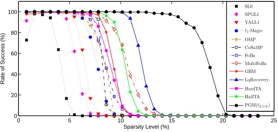
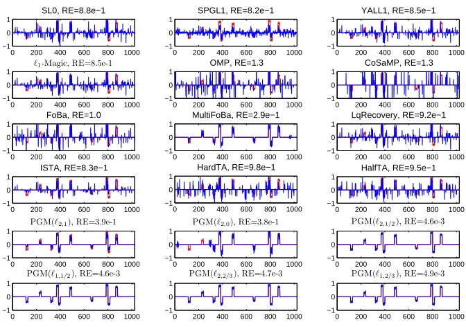
In the aspect of application, we will conduct some numerical experiments on both simu-lated data and real data in gene transcriptional regulation to demonstrate the performance of the proposed proximal gradient method. From the numerical results, it is demonstrated that the `p,1/2 regularization is the best one among the `p,q regularizations for q ∈ [0,1],
and it outperforms the`p,1 and `p,0 regularizations on both accuracy and robustness. This
observation is consistent with several previous numerical studies on the `p regularization
problem; see Chartrand and Staneva (2008); Xu et al. (2012). It is also illustrated from the
numerical results that the proximal gradient method (`2,1/2) outperforms most solvers in
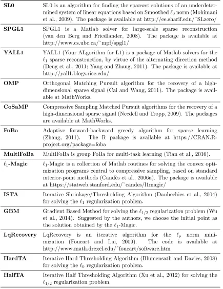
group sparse learning, such as OMP (Cai and Wang, 2011), FoBa (Zhang, 2011),`1-Magic
(Cand`es et al., 2006a), ISTA (Daubechies et al., 2004), YALL1 (Yang and Zhang, 2011) etc. The R package of the proximal gradient method for solving group sparse optimization, named GSparO in CRAN, is available at https://CRAN.R-project.org/package=GSparO
1.5 Main Contributions
This paper is to investigate the group sparse optimization under a unified framework of the
`p,q regularization problem (4). In this paper, we establish the oracle property and
recov-ery bound, design an efficient numerical method for problem (4), and apply the proposed method to solve the problem of gene transcriptional regulation. The main contributions are presented as follows.
(i) We establish the following global recovery bound for the `p,q regularization problem
(4) under the (p, q)-GREC:
kx∗−x¯k22 ≤ (
O(λ2−2qS), 2K−1q= 1,
O(λ2−2qS
3−q
2−q), 2K−1q >1,
where ¯x is a solution of Ax=b,S:=kx¯kp,0 is the group sparsity, 0< q≤1≤p≤2,
x∗ is any point in the level set levF(¯x) of problem (4), and K is the smallest integer
such that 2K−1q≥1.
(ii) By virtue of the variational analysis technique, for all the`p,qregularization problems,
we establish a uniform local recovery bound
kx∗p,q(λ)−x¯k2
2≤ O(λ2S) for small λ,
where 0< q <1≤pand x∗
p,q(λ) is a local optimal solution of problem (4) (near ¯x).
(iii) We present the analytical formulae for the proximal optimization subproblems of spe-cific `p,q regularizations when p = 1,2 and q = 0,1/2,2/3,1. Moreover, we prove
that any sequence {xk}, generated by proximal gradient method for solving the `
1,q
regularization problem, linearly converges to a local minimum x∗ under some mild
conditions, that is, there exist N ∈N,C >0 andη ∈(0,1) such that
F(xk)−F(x∗)≤Cηk and kxk−x∗k2≤Cηk for any k≥N.
(iv) Our numerical experiments show that, measured by the biological golden standards, the accuracy of the gene regulation networks forecasting can be improved by exploiting the group structure of TF complexes. The successful application of group sparse optimization to gene transcriptional regulation will facilitate biologists to study the gene regulation of higher model organisms in a genome-wide scale.
1.6 The Organization of This Paper
This paper is organized as follows. In section 2, we introduce the notions of q-REC and
GREC, and establish the oracle property and (global and local) recovery bounds for the`p,q
regularization problem. In section 3, we apply the proximal gradient method to solve the
group sparse optimization using different types of `p,q regularization, and investigate the
local linear convergence rate of the resulting proximal gradient method. Finally, section 4 exhibits the numerical results on both simulated data and real data in gene transcriptional regulation.
2. Global and Local Recovery Bounds
This section is devoted to the study of the oracle property and (global and local) recovery
bounds for the `p,q regularization problem (4). To this end, we first present some basic
inequalities of `p norm and introduce the notions of RECs, as well as their relationships.
The notations adopted in this paper are described as follows. We let the lowercase letters x, y, z denote the vectors, calligraphic letters I, T,S,J, N denote the index sets,
capital letters N, S denote the numbers of groups in the index sets. In particular, we use
Gi to denote the index set corresponding to the i-th group andGS to denote the index set
{Gi : i ∈ S}. For x ∈ Rn and T ⊆ {1, . . . , n}, we use xT to denote the subvector of x
corresponding toT. We use sign :R→Rto denote the signum function, defined by
sign(t) =
1, t >0,
0, t= 0,
Throughout this paper, we assume that the group sparse optimization problem is of the group structure described as follows. Let x := (x>G1,· · · , x>Gr)> represent the group structure of x, where {xGi ∈ R
ni : i = 1,· · ·, r} is the grouping of x, Pr
i=1ni = n and nmax:= max{ni:i∈ {1, . . . , r}}. For a groupxGi, we usexGi = 0 (reps. xGi 6= 0,xGi 6=a0)
to denote a zero (reps. nonzero, active) group, where xGi = 0 means that xj = 0 for all
j∈ Gi;xGi 6= 0 means that xj 6= 0 for some j ∈ Gi; andxGi 6=a 0 means thatxj 6= 0 for all
j∈ Gi. It is trivial to see that
xGi 6=a0 ⇒ xGi 6= 0.
For this group structure and p >0, the `p,q norm ofx is defined by
kxkp,q=
( (Pr
i=1kxGik
q
p)1/q, q >0,
Pr
i=1kxGik 0
p, q = 0,
(6)
which proposes the`p norm for each group and then processes the`q norm for the resulting
vector. When p = q, the `p,q norm coincides with the `p norm, that is, kxkp,p = kxkp.
Furthermore, all `p,0 norms share the same formula, that is, kxkp,0 =kxk2,0 for allp > 0.
In particular, when the grouping structure is degenerated to the individual feature level, that is, ifnmax= 1 or n=r, we havekxkp,q=kxkq for all p >0 andq >0.
Moreover, we assume that A andb in (4) are related by a linear model (noiseless)
b=Ax.¯
LetS :={i∈ {1, . . . , r}: ¯xGi 6= 0}be the index set of nonzero groups of ¯x,S
c:={1, . . . , r}\
S be the complement ofS,S :=|S|be the group sparsity of ¯x, and na:=Pi∈Sni.
2.1 Inequalities of `p,q Norm
We begin with some basic inequalities of the `p and `p,q norms, which will be useful in the
later discussion of RECs and recovery bounds. First, we recall the following well-known inequality
n
X
i=1
|xi|γ2
!1/γ2 ≤
n
X
i=1
|xi|γ1
!1/γ1
if 0< γ1≤γ2, (7)
or equivalently (x= (x1, x2, . . . , xn)>),
kxkγ2 ≤ kxkγ1 if 0< γ1 ≤γ2.
The following lemma improves Huang and Yang (2003, lem. 4.1) and extends to the`p,q
norm. It will be useful in providing a shaper global recovery bound (see Theorem 9 later).
Lemma 1 Let 0< q≤p≤2, x∈Rn and K be the smallest integer such that 2K−1q≥1.
Then the following relations hold.
(i) kxkqq ≤n1−2
−K
kxkq2. (ii) kxkqp,q ≤r1−2
−K
Proof (i) Repeatedly using the property that kxk1 ≤√nkxk2, one has that
kxkq q≤ √ n n X i=1
|xi|2q
!1/2
≤ · · · ≤n12+···+ 1
2K
n
X
i=1
|xi|2
Kq
!2−K .
Since 2K−1q ≥1, by (7), we obtain that
n
X
i=1
|xi|2
Kq
!2−K =
n
X
i=1
(|xi|2)2
K−1q
! 1
2K−1q
q 2 ≤ n X i=1
|xi|2
!q/2
=kxkq2.
Therefore, we arrive at the conclusion that
kxkqq≤n1−2−Kkxkq2. (ii) By (6), it is a direct consequence of (i).
For example, if q = 1, then K = 1; if q = 12 or 23, then K = 2. The following lemma
describes the triangle inequality of k · kqp,q.
Lemma 2 Let 0< q≤1≤p and x, y∈Rn. Then
kxkq
p,q− kykqp,q≤ kx−ykqp,q.
Proof By the subadditivity of the `p norm and (7), it is easy to see that
kxGik
q
p− kyGik
q
p≤ kxGi−yGik
q
p, fori= 1, . . . , r.
Consequently, the conclusion directly follows from (6).
The following lemma will be beneficial to studying properties of the lower-order REC in Proposition 5 later.
Lemma 3 Let γ ≥ 1, and two finite sequences {yi :i ∈ I} and {xj :j ∈ J } satisfy that
yi ≥xj ≥0 for all(i, j)∈ I × J. If
P
i∈Iyi ≥
P
j∈J xj, then
P
i∈Iy
γ i ≥
P
j∈Jx
γ j.
Proof Set ¯y := 1 |I|
P
i∈Iyi and α:= mini∈Iyi. By Huang and Yang (2003, lem. 4.1), one
has that
X
i∈I
yiγ≥ 1 |I|γ−1
X
i∈I
yi
!γ
=|I|y¯γ. (8)
On the other hand, letM ∈N andβ ∈[0, α) be such that Pj∈J xj =M α+β. Observing
that γ ≥ 1 and 0 ≤ xj ≤ α for all j ∈ J, we obtain that xγj ≤ xjαγ−1, and thus,
P
j∈J x
γ
j ≤M αγ+αγ−1β. By (8), it remains to show that
|I|y¯γ ≥M αγ+αγ−1β. (9)
If |I|> M, the relation (9) is trivial since ¯y ≥α > β; otherwise, |I| ≤ M, from the facts that|I|y¯≥M α+β (that is, P
i∈Iyi ≥Pj∈J xj) and thatγ ≥1, it follows that
2.2 Group Restricted Eigenvalue Conditions
This subsection aims at the development of the critical conditions on the matrixAto
guar-antee the oracle property and the global recovery bound of the `p,q regularization problem
(4). In particular, we will focus on the restricted eigenvalue condition (REC), and extend it to the lower-order setting and equip it with the group structure.
In the scenario of sparse optimization, given the sparsity level s, it is always assumed
that the 2s-sparse minimal eigenvalue of A>A is positive (see Bickel et al., 2009; Bunea
et al., 2007; Meinshausen and Yu, 2009), that is,
φmin(2s) := min kxk0≤2s
x>A>Ax
x>x >0, (10)
which is the minimal eigenvalue of any 2s×2sdimensional submatrix. It is well-known that
the solution at sparsity levelsof the linear system Ax=bis unique if the condition (10) is
satisfied; otherwise, assume that there are two distinct vectors ˆx and ˜x such thatAxˆ=Ax˜ and kxˆk0 = kx˜k0 = s. Then x := ˆx−x˜ is a vector such that Ax = 0 and kxk0 ≤ 2s,
and thus φmin(2s) = 0, which is contradict with (10). Therefore, if the 2s-sparse minimal
eigenvalue of A>A is zero (that is, φmin(2s) = 0), one has no hope of recovering the true
sparse solution from noisy observations.
However, only condition (10) is not enough and some further condition is required to maintain the nice recovery of regularization problems; see Bickel et al. (2009); Bunea et al.
(2007); Meinshausen and Yu (2009); van de Geer and B¨uhlmann (2009); Zhang (2009)
and references therein. For example, the REC was introduced in Bickel et al. (2009) to
investigate the`2 consistency of the `1 regularization problem (Lasso), where the minimum
in (10) is replaced by a minimum over a restricted set of vectors measured by an `1 norm
inequality and the denominator is replaced by the`2 norm of only a part ofx.
We now introduce the notion of the lower-order REC. Note that the residual ˆx :=
x∗(`q)−x¯, wherex∗(`q) is an optimal solution of the `q regularization problem and ¯x is a
sparse solution of Ax=b, of the `q regularization problem always satisfies
kxˆSckq≤ kxˆSkq, (11)
whereS is the support of ¯x. Thus we introduce a lower-order REC, where the minimum is
taken over a restricted set measured by an`q norm inequality such as (11), for establishing
the global recovery bound of the `q regularization problem. Givens≤tn,x ∈Rn and
I ⊆ {1, . . . , n}, we denote by I(x;t) the subset of {1, . . . , n} corresponding to the first t largest coordinates in absolute value ofx inIc.
Definition 4 Let 0 ≤ q ≤ 1. The q-restricted eigenvalue condition relative to (s, t) (q
-REC(s, t))is said to be satisfied if
φq(s, t) := min
kAxk2
kxTk2
:|I| ≤s,kxIckq ≤ kxIkq,T =I(x;t)∪ I
>0.
The q-REC describes a kind of restricted positive definiteness ofA>A, which is valid only
for the vectors satisfying the relation measured by an `q norm. The q-REC presents a
(a) REC (b) 1/2-REC (c) 0-REC
Figure 1: The geometric interpretation of the RECs: the gray regions show the feasible sets Cq(s) (q= 1,1/2,0). Theq-REC holds if and only if the null space ofAdoes not
intersect the gray region.
definition that 1-REC reduces to the classical REC (Bickel et al., 2009), and thatφmin(2s) =
φ2
0(s, s), and thus
(10) ⇔ 0-REC(s, s) is satisfied.
It is well-known in the literature that the 1-REC is a stronger condition than the 0-REC
(10). A natural question arises what are the relationships between the generalq-RECs. To
answer this question, associated with theq-REC, we consider the feasible set
Cq(s) :={x∈Rn:kxIckq≤ kxIkq for some|I| ≤s},
which is a cone. Since the objective function associated with the q-REC is homogeneous,
the q-REC(s, t) says that the null space ofA does not cross overCq(s). Figure 1 presents
the geometric interpretation of theq-RECs. It is shown in Figure 1 thatC0(s)⊆C1/2(s)⊆
C1(s), and thus
1-REC ⇒ 1/2-REC ⇒ 0-REC.
It is also observed from Figure 1 that the gap between the 1-REC and 1/2-REC and that between 1/2-REC and 0-REC are the matrices whose null spaces fall in the cones of C1(s)\C1/2(s) andC1/2(s)\C0(s), respectively.
We now provide a rigorous proof in the following proposition to identify the relationship between the feasible setsCq(s) and between the generalq-RECs: the lower theq, the smaller
the coneCq(s), and the weaker the q-REC.
Proposition 5 Let 0≤q1 ≤q2≤1 and1≤s≤tn. Then the following statements are
true:
(i) Cq1(s)⊆Cq2(s), and
(ii) if the q2-REC(s, t) holds, then the q1-REC(s, t) holds.
Proof (i) Fixx∈Cq1(s). We useI∗to denote the index set of the firstslargest coordinates in absolute value ofx. Sincex ∈Cq1(s), it follows that kxI∗ckq1 ≤ kxI∗kq1 (|I∗| ≤sdue to
the construction of I∗). By Lemma 3 (takingγ =q2/q1), one has that
kxIc
that is,x∈Cq2(s). Hence it follows that Cq1(s)⊆Cq2(s).
(ii) As proved by (i) that Cq1(s)⊆Cq2(s), by the definition ofq-REC, it follows that
φq1(s, t)≥φq2(s, t)>0.
The proof is complete.
To the best of our knowledge, this is the first work on introducing the lower-order REC and establishing the relationship of the lower-order RECs. In the following, we provide a counter example to show that the reverse of Proposition 5 is not true.
Example 1 (A matrix satisfying 1/2-REC but not REC) Consider the matrix
A:=
a a+c a−c
˜
a ˜a−˜c ˜a+ ˜c
∈R2×3,
where a > c >0 and a >˜ c >˜ 0. This matrix A does not satisfy the REC(1,1). Indeed, by
letting J ={1} andx= (2,−1,−1)>, we have Ax= 0 and thus φ(1,1) = 0.
Below, we claim thatA satisfies the 1/2-REC(1,1). It suffices to show thatφ1/2(1,1)>
0. Let x= (x1, x2, x3)> satisfy the constraint associated with1/2-REC(1,1). As s= 1, the
deduction is divided into the following three cases.
(i) J ={1}. Then
|x1| ≥ kxJck1/2 =|x2|+|x3|+ 2|x2|1/2|x3|1/2. (12)
Without loss of generality, we assume|x1| ≥ |x2| ≥ |x3|. Hence,T ={1,2} and
kAxk2
kxTk2 ≥
min{a,˜a}|x1+x2+x3|+ min{c,˜c}|x2−x3|
|x1|+|x2|
. (13)
If |x2| ≤ 13|x1|, (13)reduces to
kAxk2
kxTk2 ≥
min{a,˜a} 3 |x1| 4 3|x1|
= min{a,a˜}
4 . (14)
If |x2| ≥ 13|x1|, substituting (12) into (13), one has that
kAxk2
kxTk2 ≥
(min{c,˜c}
8 , |x3| ≤ 1 2|x2|, min{a,˜a}
4 , |x3| ≥ 1 2|x2|.
(15)
(ii) J ={2}. SinceT ={2,1}or{2,3}, it follows from Huang and Yang (2003, lem. 4.1)
that
|x2| ≥ kxJck1/2≥ |x1|+|x3|. (16)
Thus, it is easy to verify thatkxTk2 ≤2|x2|and that
kAxk2
kxTk2 ≥
|ax1+ (a+c)x2+ (a−c)x3|
2|x2|
= |a(x1+x2+
a−c
a x3) +cx2|
2|x2| ≥
c
2, (17)
(iii) J ={3}. Similar to the deduction of (ii), one has that
kAxk2
kxTk2 ≥
|˜ax1+ (˜a−c˜)x2+ (˜a+ ˜c)x3|
2|x3| ≥
˜ c
2. (18)
Therefore, by (14)-(15) and (17)-(18), we conclude that φ1/2(1,1) ≥ 1
8min{c,˜c} >0, and
thus, the matrix A satisfies the 1/2-REC(1,1).
In order to establish the oracle property and the global recovery bound for the`p,q
regu-larization problem, we further introduce the notion of group restricted eigenvalue condition
(GREC). Given S ≤ N r, x ∈ Rn and J ⊆ {1, . . . , r}, we use ranki(x) to denote the
rank of kxGikp among {kxGjkp : j ∈ J
c} (in a decreasing order), J(x;N) to denote the
index set of the firstN largest groups in the value ofkxGikp among{kxGjkp :j∈ J
c}, that
is,
J(x;N) :={i∈ Jc: ranki(x)∈ {1, . . . , N}}.
Furthermore, by lettingR:=dr−|J |N e, we denote
Jk(x;N) :=
{i∈ Jc: rank
i(x)∈ {kN+ 1, . . . ,(k+ 1)N}}, k= 1, . . . , R−1,
{i∈ Jc: rank
i(x)∈ {RN+ 1, . . . , r− |J |}}, k=R.
(19)
Note that the residual ˆx:=x∗(`p,q)−x¯of the`p,qregularization problem always satisfies
kxˆGSckp,q≤ kxˆGSkp,q. Thus we introduce the notion of GREC, where the minimum is taken
over a restricted set measured by an`p,q norm inequality, as follows.
Definition 6 Let 0 < q ≤p ≤2. The (p, q)-group restricted eigenvalue condition relative
to (S, N) ((p, q)-GREC(S, N))is said to be satisfied if
φp,q(S, N) := min
kAxk2
kxGNkp,2
:|J | ≤S,kxGJckp,q≤ kxGJkp,q,N =J(x;N)∪ J
>0.
The (p, q)-GREC extends the q-REC to the setting equipping with a pre-defined group
structure. Handling the components in each group as one element, the (p, q)-GREC admits
the fewer degree of freedom, which is S (abouts/nmax), on its associated constraint than
that of the q-REC, and thus it characterizes a weaker condition than the q-REC. For
example, the 0-REC(s, s) is to indicate the restricted positive definiteness ofA>A, which is valid only for the vectors whose cardinality is less than 2s; while the (p,0)-GREC(S, S) is to describe the restricted positive definiteness ofA>Aon any 2S-group support, whose degree
of freedom is much less than the 2s-support. Thus the (p,0)-GREC(S, S) provides a broader
condition than the 0-REC(s, s). Similar to the proof of Proposition 5, we can show that if
0 ≤q1 ≤q2 ≤1 ≤p ≤2 and the (p, q2)-GREC(S, N) holds, then the (p, q1)-GREC(S, N)
also holds.
We end this subsection by providing the following lemma, which will be useful in
estab-lishing the global recovery bound for the `p,q regularization problem in Theorem 9.
Lemma 7 Let 0< q ≤1≤p, τ ≥1 and x∈Rn, N :=J(x;N)∪ J and Jk :=Jk(x;N)
for k= 1, . . . , R. Then the following inequalities hold
kxGNckp,τ ≤ R
X
k=1
kxGJkkp,τ ≤N
1
τ−
1
qkxG
Proof By the definition of Jk (19), for eachj∈ Jk, one has that
kxGjkp ≤ kxGikp, for each i∈ Jk−1,
and thus
kxGjk
q p ≤
1 N
X
i∈Jk−1 kxGik
q p =
1
NkxGJk−1k
q p,q.
Consequently, we obtain that
kxGJkk
τ p,τ =
X
i∈Jk
kxGik
τ
p ≤N1−τ /qkxGJk−1k
τ p,q.
Further by Huang and Yang (2003, lem. 4.1) (τ ≥1 andq≤1), it follows that
kxGNckp,τ =
PR
k=1
P
i∈JkkxGik
τ p
1/τ
≤PR
k=1kxGJkkp,τ
≤Nτ1−
1
q PR
k=1kxGJk−1kp,q
≤Nτ1−
1
qkxG
Jckp,q.
The proof is complete.
2.3 Global Recovery Bound
In recent years, many articles have been devoted to establishing the oracle property and
the global recovery bound for the`1 regularization problem (1) under the RIP or REC; see
Bickel et al. (2009); Meinshausen and Yu (2009); van de Geer and B¨uhlmann (2009); Zhang
(2009). However, to the best of our knowledge, there is few paper devoted to investigating these properties for the lower-order regularization problem.
In the preceding subsections, we have introduced the general notion of (p, q)-GREC.
Under the (p, q)-GREC(S, S), the solution ofAx=bwith group sparsity beingS is unique.
In this subsection, we will present the oracle property and the global recovery bound for
the`p,q regularization problem (4) under the (p, q)-GREC. The oracle property provides an
upper bound on the squares error of the linear system and the violation of the true nonzero groups for each point in the level set of the objective function of problem (4)
levF(¯x) :={x∈Rn:kAx−bk22+λkxkqp,q≤λkx¯kqp,q}.
Proposition 8 Let 0< q≤1≤p,S >0 and let the (p, q)-GREC(S, S) hold. Let x¯ be the
unique solution of Ax = b at a group sparsity level S, and S be the index set of nonzero
groups ofx¯. LetK be the smallest integer such that2K−1q ≥1. Then, for anyx∗∈lev
F(¯x),
the following oracle inequality holds
kAx∗−Ax¯k22+λkx∗GSck
q p,q ≤λ
2
2−qS(1−2
−K) 2
2−q/φ
2q
2−q
p,q (S, S). (20)
Moreover, letting N∗:=S ∪ S(x∗;S), we have
kx∗GN∗ −x¯GN∗k2p,2 ≤λ
2
2−qS(1−2
−K) 2
2−q/φ
4
2−q
Proof Letx∗ ∈lev
F(¯x). That is,kAx∗−bk22+λkx∗k
q
p,q≤λkx¯kqp,q. By Lemmas 1(ii) and
2, one has that
kAx∗−Ax¯k2
2+λkx∗GSck
q
p,q ≤λkx¯GSk
q
p,q−λkx∗GSk
q p,q
≤λkx¯GS −x
∗ GSk
q p,q
≤λS1−2−K
kx¯GS −x
∗ GSk
q p,2.
(21)
Noting that
kx∗GSc−x¯GSckqp,q− kx∗GS−x¯GSk
q
p,q≤ kx∗GSck
q
p,q−(kx¯GSk
q
p,q− kx∗GSk
q
p,q) =kx∗kqp,q− kx¯kqp,q≤0.
Then the (p, q)-GREC(S, S) implies that
kx¯GS−x
∗
GSkp,2 ≤ kAx
∗
−Ax¯k2/φp,q(S, S).
This, together with (21), yields that
kAx∗−Ax¯k2
2+λkx∗GSck
q
p,q≤λS1−2
−K
kAx∗−Ax¯kq2/φq
p,q(S, S), (22)
and consequently,
kAx∗−Ax¯k2 ≤λ
1
2−qS(1−2−K)/(2−q)/φ
q
2−q
p,q (S, S). (23)
Therefore, by (22) and (23), we arrive at the oracle inequality (20). Furthermore, by the definition ofN∗, the (p, q)-GREC(S, S) implies that
kx∗
GN∗−x¯GN∗k2p,2≤ kAx∗−Ax¯k22/φ2p,q(S, S)≤λ 2
2−qS(1−2
−K) 2
2−q/φ
4
2−q
p,q (S, S).
The proof is complete.
One of the main results of this section is presented as follows, where we establish the
global recovery bound for the `p,q regularization problem under the (p, q)-GREC. We will
apply oracle inequality (20) and Lemma 7 in our proof.
Theorem 9 Let 0 < q ≤ 1 ≤ p ≤ 2, S > 0 and let the (p, q)-GREC(S, S) hold. Let x¯
be the unique solution of Ax = b at a group sparsity level S, and S be the index set of
nonzero groups of x¯. Let K be the smallest integer such that 2K−1q ≥ 1. Then, for any
x∗ ∈levF(¯x), the following global recovery bound for problem (4) holds
kx∗−x¯k2 2 ≤2λ
2
2−qS
q−2
q +(1−2
−K) 4
q(2−q)/φ 4
2−q
p,q (S, S). (24)
More precisely,
kx∗−x¯k22≤ (
O(λ2−2qS), 2K−1q = 1,
O(λ2−2qS
3−q
2−q), 2K−1q >1.
Proof Let N∗ := S ∪ S(x∗;S) as in Proposition 8. Sincep≤2, it follows from Lemma 7
and Proposition 8 that
kx∗GNc
∗k
2
2≤ kx∗GNc
∗k
2
p,2≤S1−2/qkx∗GSck 2
p,q ≤λ 2
2−qS
q−2
q +(1−2
−K) 4
q(2−q)/φ 4
2−q
p,q (S, S).
Then by Proposition 8, one has that
kx∗−x¯k2
2 =kx∗GN∗−x¯GN∗k22+kx∗GNc
∗k
2 2
≤λ2−2qS(1−2
−K) 2
2−q/φ
4
2−q
p,q (S, S) +λ 2
2−qS
q−2
q +(1−2
−K) 4
q(2−q)/φ 4
2−q
p,q (S, S)
≤2λ2−2qS q−2
q +(1−2
−K) 4
q(2−q)/φ 4
2−q
p,q (S, S),
where the last inequality follows from the fact that 2K−1q ≥ 1. This proves (24). In
particular, if 2K−1q= 1, then q−2
q + 1−2
−K 4
q(2−q) = 1 and thus
kx∗−x¯k22 ≤ O(λ2−2qS).
If 2K−1q >1, then 2K−2q <1. Hence, q−2
q + 1−2
−K 4
q(2−q) < 3−q
2−q, and consequently
kx∗−x¯k2
2 ≤ O(λ
2
2−qS
3−q
2−q).
Hence (25) is obtained. The proof is complete.
The global recovery bound (25) is deduced under general (p, q)-GREC(S, S), which is
weaker than the REC as used in van de Geer and B¨uhlmann (2009). It shows that the sparse
solution ¯x may be recovered by any pointx∗ in the level set levF(¯x), in particular, when x∗
is a global optimal solution of problem (4), as long asλis sufficiently small. It is well-known
that whenp= 2 andq = 1, convex regularization problem (4) is numerically intractable for
finding the sparse solution and that when q <1 finding a point in the nonconvex level set
levF(¯x) is equivalent to finding a global minimum of minimizing the indicator function of
the nonconvex level set, which is NP-hard. Thus Theorem 9 is only a theoretical result and does not provide any insight for the numerical computation of a sparse solution by virtue of problem (4). We will design a proximal gradient method in section 3, test its numerical
efficiency and provide some general guidance on which q is more attractive in practical
applications in section 4.
To conclude this subsection, we illustrate by an example in which (24) does not hold
when q = 1, but it does and is also tight when q = 1
2. We will testify the recovery bound
O(λ4/3S) in (24) whenq = 1
2 by using a global optimization method.
Example 2 By letting a= ˜a= 2 and c = ˜c = 1 in Example 1, we consider the following matrix:
A:=
2 3 1 2 1 3
.
We set b := (2,2)> and then a true solution of Ax = b is x¯ := (1,0,0)>. Denoting
x:= (x1, x2, x3)>, the objective function associated with the`1 regularization problem (1)is
F(x) :=kAx−bk2
2+λkxk1
Letx∗(`
1) := (x∗1, x∗2, x∗3)> be an optimal solution of problem (1). Without loss of generality,
we assume λ≤1. The necessary condition of x∗(`1) being an optimal solution of problem
(1) is0∈∂F(x∗(`1)), that is,
0∈16x∗1+ 16x∗2+ 16x∗3−16 +λ∂|x∗1|, (26a)
0∈16x∗1+ 20x∗2+ 12x∗3−16 +λ∂|x∗2|, (26b)
0∈16x∗1+ 12x∗2+ 20x∗3−16 +λ∂|x∗3|, (26c)
where ∂|µ|:=
sign(µ), µ6= 0,
[−1,1], µ= 0.
We first show that x∗i ≥ 0 for i = 1,2,3 by contradiction. Indeed, if x∗1 < 0, (26a)
reduces to
16x∗1+ 16x∗2+ 16x∗3−16 =λ.
Summing (26b) and (26c), we further have
λ= 16x∗1+ 16x2∗+ 16x∗3−16∈ −λ 2(∂|x
∗ 2|+∂|x
∗ 3|),
which implies thatx∗2 ≤0 andx∗3 ≤0. Hence, it follows thatF(x∗)> F(0), which indicates
thatx∗ is not an optimal solution of problem (1), and thus, x∗1 <0is impossible. Similarly,
we can show that x∗
2 ≥0 and x∗3 ≥0.
Next, we find the optimal solution x∗(`1) by only considering x∗(`1) ≥ 0. It is easy
to obtain that the solution of (26) and the corresponding objective value associated with
problem (1)can be represented respectively by
x∗1 = 1− λ 16 −2x
∗
3, x∗2=x∗3
0≤x∗3 ≤ 1
2−
λ 32
, and F(x∗(`1)) =λ−
λ2
32.
Hence, x∗(`1) := 0,21 −32λ,12 −32λ
>
is an optimal solution of problem (1). The estimated
error for this x∗(`1) is
kx∗(`1)−x¯k22= 1 +
1 2
1− λ
16
2
>1,
which does not meet the recovery bound (25) for any λ≤1.
It is revealed from Example 1 that this matrix A satisfies the 1/2-REC(1,1). Then
the hypothesis of Theorem 9 is verified, and thus, Theorem 9 is applicable to establishing
the recovery bound (25) for the `1/2 regularization problem. Although we cannot obtain
the closed-form solution of this nonconvex `1/2 regularization problem, as it is of only
3-dimensions, we can apply a global optimization method, the filled function method (Ge,
1990), to find the global optimal solution x∗(`1/2) and thus to testify the recovery bound
(25). This is done by computing the`1/2 regularization problem for manyλto plot the curve
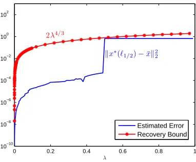
kx∗(`1/2)−x¯k22. Figure 2 illustrates the variation of the estimated errorkx∗(`1/2)−x¯k22 and
the bound 2λ4/3 (that is the right-hand side of (24), where S = 1 and φ
1/2(1,1)≤ 1 (see
Example 1)), when varying the regularization parameter λ from 10−8 to 1. It is illustrated
0 0.2 0.4 0.6 0.8 1 10−10
10−8 10−6 10−4 10−2 100 102
λ kx∗(ℓ
1/2)−¯xk22 2λ4/3
Estimated Error Recovery Bound
Figure 2: The illustration of the recovery bound (24) and estimated error.
2.4 Local Recovery Bound
In the preceding subsection, we provided the global analysis of the recovery bound for the
`p,q regularization problem under the (p, q)-GREC; see Theorem 9. One can also observe
from Figure 2 that the global recovery bound (25) is tight for the`1/2regularization problem
as the curves come together at λ ' 0.5, but there is still a big gap for the improvement
when λis small.
This subsection is devoted to providing a local analysis of the recovery bound for the
`p,q regularization problem by virtue of the variational analysis technique (Rockafellar and
Wets, 1998). For x ∈Rn and δ ∈ R+, we use B(x, δ) to denote the open ball of radius δ
centered at x. For a lower semi-continuous (lsc) function f :Rn → R and x, w ∈Rn, the
subderivative of f atx along the directionwis defined by
df(¯x)(w) := lim inf
τ↓0, w0→w
f(¯x+τ w0)−f(¯x)
τ .
To begin with, we show in the following lemma a significant advantage of lower-order
regu-larization over the `1 regularization: the lower-order regularization term can easily induce
the sparsity of the local minimum.
Lemma 10 Let 0 < q <1≤p. Let f :Rn → R be a lsc function satisfying df(0)(0) = 0.
Then the function F := f +λk · kqp,q has a local minimum at 0 with the first-order growth
condition being fulfilled, that is, there exist some >0 and δ >0 such that
F(x)≥F(0) +kxk2 for anyx∈B(0, δ).
Proof Letϕ:=λk · kqp,q and thenF =f+ϕ. Sinceϕis grouped separable, by Rockafellar
and Wets (1998, prop. 10.5), it follows from the definition that dϕ(0) = δ{0}, where δX is
the indicator function of X. Applying Rockafellar and Wets (1998, prop. 10.9), it follows
that
By the assumption that f is finite and df(0)(0) = 0, its subderivative df(0) is proper
(see Rockafellar and Wets, 1998, ex. 3.19). Noting that df(0)(0) = 0, we obtain that
df(0) +δ{0} = δ{0}. This, together with (27), yields that dF(0) ≥ δ{0}. Therefore, by
definition, there exist some >0 and δ >0 such that
F(x)≥F(0) +kxk2 for any x∈B(0, δ).
The proof is complete.
With the help of the above lemma, we can present in the following a local version of the recovery bound. This is done by constructing a path of local minima depending on
the regularization parameter λ for the regularization problem, which starts from a sparse
solution of the original problem and shares the same support as this sparse solution has,
resulting in a sharper bound in terms of λ2.
Theorem 11 Let x¯ be a solution of Ax = b, S be the group sparsity of x¯, and B be
a submatrix of A consisting of its columns corresponding to the active components of x¯.
Suppose that any nonzero group of x¯ is active, and that the columns of A corresponding to
the active components of x¯ are linearly independent. Let 0 < q <1 ≤p. Then there exist
κ >0 and a path of local minima of problem (4), x∗(λ), such that
kx∗(λ)−x¯k22≤λ2q2Sk(B>B)−1k2 max
¯
xGi6=0
kx¯Gik
2(q−p)
p kx¯Gik 2p−2 2p−2
for anyλ < κ.
Proof Without loss of generality, we let ¯x be of structure ¯x= (¯z>,0)> with
¯
z= (¯x>G1, . . . ,x¯>G
S)
> and ¯x
Gi 6=a0 for i= 1, . . . , S,
and let sbe the sparsity of ¯x. Let A = (B, D) with B being the submatrix involving the
firstscolumns of A(corresponding to the active components of ¯x). By the assumption, we
have that B is of full column rank and thus B>B is invertible. In this setting, the linear
relationAx¯=breduces to Bz¯=b. The proof of this theorem is divided into the following three steps:
(a) construct a smooth path from ¯x by the implicit function theorem;
(b) validate that every point of the constructed path is a local minimum of (4); and
(c) establish the recovery bound for the constructed path.
First, to show (a), we defineH :Rs+1→Rs by
H(z, λ) = 2B>(Bz−b) +λq
kzG1k q−p p σ(zG1)
.. . kzGSk
q−p p σ(zGS)
,
whereσ(zGi) = vector |zj|
p−1sign(z
j)
Gi, denoting a vector consisting of|zj|
p−1sign(z
j) for
and thusH is smooth onB(¯z,¯δ)×R. Note thatH(¯z,0) = 0 and ∂H∂z(¯z,0) = 2B>B. By the
implicit function theorem (Rudin, 1976), there exist some κ > 0, δ ∈ (0,δ¯) and a unique
smooth function ξ: (−κ, κ)→B(¯z, δ) such that
{(z, λ)∈B(¯z,δ¯)×(−κ, κ) :H(z, λ) = 0}={(ξ(λ), λ) :λ∈(−κ, κ)}, (28)
and
dξ dλ =−q
2B
>B+λq
M1 0 0
0 . .. 0
0 0 MS
−1
kξ(λ)G1k q−p
p σ(ξ(λ)G1) ..
. kξ(λ)GSk
q−p
p σ(ξ(λ)GS)
, (29)
whereMi for each i= 1, . . . , S is denoted by
Mi = (q−p)kξ(λ)Gik
q−2p
p (σ(ξ(λ)Gi))(σ(ξ(λ)Gi)) >
+ (p−1)kξ(λ)Gik
q−p
p diag |ξ(λ)j|p−2
,
and diag |ξ(λ)j|p−2
denotes a diagonal matrix generated by vector |ξ(λ)j|p−2
. Thus, by (28) and (29), we have constructed a smooth pathξ(λ) near ¯z,λ∈(−κ, κ), such that
2B>(Bξ(λ)−b) +λq
kξ(λ)G1k q−p
p σ(ξ(λ)G1) ..
. kξ(λ)GSk
q−p
p σ(ξ(λ)GS)
= 0 (30)
and
2B>B+λq
M1 0 0
0 . .. 0
0 0 MS
0. (31)
This shows that (a) is done as desired.
For fixed λ ∈ (−κ, κ), let x∗(λ) := (ξ(λ)>,0)>. To verify (b), we prove that x∗(λ),
with ξ(λ) satisfying (30) and (31), is a local minimum of problem (4). Let h : Rs → R
be a function with h(z) := kBz −bk2
2 +λkzk
q
p,q for any z ∈ Rs. Note that h(ξ(λ)) =
kAx∗(λ)−bk2
2+λkx∗(λ)k
q
p,q and thathis smooth aroundξ(λ). By noting thatξ(λ) satisfies
(30) and (31) (the first- and second- derivative of h at ξ(λ)), one has that h satisfies the
second-order growth condition atξ(λ), that is, there exist λ >0 and δλ >0 such that
h(z)≥h(ξ(λ)) + 2λkz−ξ(λ)k22 for any z∈B(ξ(λ), δλ). (32)
In what follows, letλ >0 andδλ>0 be given as above, and select0 >0 such that
√
λ0− kBkkDk>0. (33)
According to Lemma 10 (with kD· k2
2 + 2hBξ(λ)−b, D·i −20k · k22 in place of f), there
existsδ0 >0 such that
Thus, for each x:= (z, y)∈B(ξ(λ), δλ)×B(0, δ0), it follows that
kAx−bk2
2+λkxk
q p,q
=kBz−b+Dyk2
2+λkzk
q
p,q+λkykqp,q
=kBz−bk2
2+λkzk
q
p,q+kDyk22+ 2hBz−b, Dyi+λkyk
q p,q
=h(z) +kDyk2
2+ 2hBξ(λ)−b, Dyi+λkyk
q
p,q+ 2hB(z−ξ(λ)), Dyi.
By (32) and (34), it yields that
kAx−bk2
2+λkxk
q p,q
≥h(ξ(λ)) + 2λkz−ξ(λ)k22+ 20kyk22+ 2hB(z−ξ(λ)), Dyi
≥h(ξ(λ)) + 4√λ0kz−ξ(λ)k2kyk2−2kBkkDkkz−ξ(λ)k2kyk2
=kAx∗(λ)−bk2
2+λkx∗(λ)k
q
p,q+ 2(2√λ0− kBkkDk)kz−ξ(λ)k2kyk2
≥ kAx∗(λ)−bk2
2+λkx∗(λ)k
q p,q,
where the last inequality follows from (33). Hencex∗(λ) is a local minimum of problem (4),
and (b) is verified.
Finally, we check (c) by providing an upper bound on the distance from ξ(λ) to ¯z. By
(30), one has that
ξ(λ)−¯z=−λq 2 ((B
>B)−1)
kξ(λ)G1k q−p
p σ(ξ(λ)G1) ..
. kξ(λ)GSk
q−p
p σ(ξ(λ)GS)
. (35)
Noting that {ξ(λ) : λ∈ (−κ, κ)} ⊆ B(¯z,δ¯), without loss of generality, we assume for any λ < κthat
kξ(λ)Gik 2(q−p)
p ≤2kz¯Gik 2(q−p)
p and kξ(λ)Gik 2p−2
2p−2 ≤2kz¯Gik 2p−2
2p−2 fori= 1, . . . , S
(otherwise, we choose a smaller ¯δ). Recall thatσ(ξ(λ)Gi) = vector |ξ(λ)j|
p−1sign(ξ(λ)
j)
Gi.
We obtain from (35) that
kξ(λ)−z¯k2 2 ≤
λ2q2
4 k(B
>B)−1k2PS
i=1
kξ(λ)Gik 2(q−p)
p Pj∈Gi|ξ(λ)j| 2p−2
= λ24q2k(B>B)−1k2PS
i=1
kξ(λ)Gik 2(q−p)
p kξ(λ)Gik 2p−2 2p−2
≤ λ24q2k(B
>B)−1k2S max
i=1,...,S
kξ(λ)Gik 2(q−p)
p kξ(λ)Gik 2p−2 2p−2
≤λ2q2Sk(B>B)−1k2 max
i=1,...,S
kz¯Gik
2(q−p)
p kz¯Gik 2p−2 2p−2
.
Hence we arrive at that
kx∗(λ)−x¯k2
2 =kξ(λ)−z¯k22≤λ2q2Sk(B >
B)−1k2 max ¯
xGi6=0
kx¯Gik
2(q−p)
p kx¯Gik 2p−2 2p−2
Theorem 11 provides a uniform local recovery bound for all the`p,q regularization
prob-lems (0< q <1≤p), which is
kx∗p,q(λ)−x¯k22 ≤ O(λ2S),
wherex∗p,q(λ) is a local optimal solution of problem (4) (near ¯x). This bound improves the
global recovery bound given in Theorem 9 (of orderO(λ2−2q)) and shares the same one with
the `p,1 regularization problem (group Lasso); see Blumensath and Davies (2008); van de
Geer and B¨uhlmann (2009). It is worth noting that our proof technique is not working
when q= 1 as Lemma 10 fails in this case.
3. Proximal Gradient Method for Group Sparse Optimization
Many efficient algorithms have been proposed to solve sparse optimization problems, and one of the most popular optimization algorithms is the proximal gradient method (PGM); see Beck and Teboulle (2009); Combettes and Wajs (2005); Xiao and Zhang (2013) and references therein. It was reported in Combettes and Wajs (2005) that the PGM for
solv-ing the `1 regularization problem (1) reduces to the well-known iterative soft thresholding
algorithm (ISTA), and that the ISTA has a local linear convergence rate under some as-sumptions; see Bredies and Lorenz (2008); Hale et al. (2008); Tao et al. (2016). Recently, the global convergence of the PGM for solving some types of nonconvex regularization prob-lems have been studied under the framework of the Kurdyka- Lojasiewicz theory (Attouch et al., 2010; Bolte et al., 2013), the majorization-minimization scheme (Mairal, 2013), the coordinate gradient descent method (Tseng and Yun, 2009), the general iterative shrinkage and thresholding (Gong et al., 2013) and the successive upper-bound minimization approach (Razaviyayn et al., 2013).
In this section, we apply the PGM to solve the group sparse optimization problem (4) (PGM-GSO), which is stated as follows.
Algorithm 1 (PGM-GSO) Select a stepsize v, start with an initial point x0 ∈Rn, and
generate a sequence {xk} ⊆
Rn via the iteration
zk = xk−2vA>(Axk−b), (36)
xk+1 ∈ arg min
x∈Rn
λkxkq
p,q+
1
2vkx−z kk2
2
. (37)
Global convergence of the PGM-GSO falls in the framework of the Kurdyka- Lojasiewicz theory (see Attouch et al., 2010). In particular, following from Bolte et al. (2013, prop. 3), the sequence generated by the PGM-GSO converges to a critical point, especially a global
minimum whenq ≥1 and a local minimum whenq= 0 (inspired by the idea in Blumensath
and Davies, 2008), as summarized as follows.
Theorem 12 Let p ≥ 1, and let {xk} be a sequence generated by the PGM-GSO with v < 1
2kAk −2
2 . Then the following statements hold:
(ii) if q= 0, then {xk} converges to a local minimum of problem (4), and
(iii) if 0< q <1, then {xk} converges to a critical point 1 of problem (4).
Although the global convergence of the PGM-GSO has been provided in Theorem 12, some important issues of the PGM-GSO have not been discovered yet. The section is to continue the development of the PGM-GSO, concentrating on its efficiency and applicability. In particular, we will establish the local convergence rate of the PGM-GSO under some mild
conditions, and derive the analytical solutions of subproblem (37) for some specificpand q.
3.1 Local Linear Convergence Rate
In this subsection, we establish the local linear convergence rate of the PGM-GSO for the
case whenp= 1 and 0< q <1. For the reminder of this subsection, we always assume that
p= 1 and 0< q <1.
To begin with, by virtue of the second-order necessary condition of subproblem (37), the
following lemma provides a lower bound for nonzero groups of sequence {xk}generated by
the PGM-GSO and shows that the index set of nonzero groups of{xk} maintains constant
for largek.
Lemma 13 Let K = (vλq(1−q))2−1q, and let {xk} be a sequence generated by the
PGM-GSO with v < 1
2kAk −2
2 . Then the following statements hold:
(i) For any iand k, if xk
Gi 6= 0, then kx
k
Gik1 ≥K.
(ii) xk shares the same index set of nonzero groups for large k, that is, there existN ∈
N
andI ⊆ {1, . . . , r} such that
xk
Gi 6= 0, i∈ I,
xk
Gi = 0, i /∈ I,
for all k≥N .
Proof (i) For each group xk
Gi, by (37), one has that
xkGi ∈arg min
x∈Rni
λkxkq1+ 1
2vkx−z k−1 Gi k
2 2
. (38)
Ifxk
Gi 6= 0, we defineA
k
i :={j∈ Gi:xkj = 06 } andaki :=|Aki|. Without loss of generality, we
assume that the firstak
i components ofxkGi are nonzeros. Then (38) implies that
xkGi ∈ arg min
x∈Raki×{0}
λkxkq1+ 1
2vkx−z k−1 Gi k
2 2
.
Its second-order necessary condition says that
1 vI
k
i +λq(q−1)Mik0,
whereIk
i is the identity matrix inRa
k
i×aki andMk
i =kxkAk ik
q−2
1 (sign(xkAk i
))(sign(xk
Ak i
))>. Let
ebe the first column ofIk
i. Then, we obtain that
1 ve
>
Iike+λq(q−1)e>Mike≥0,
that is,
1
v +λq(q−1)kx k
Ak ik
q−2 1 ≥0.
Consequently, it implies that
kxkGik1=kx
k
Ak
ik1 ≥(vλq(1−q))
1
2−q =K.
Hence, it completes the proof of (i).
(ii) Recall from Theorem 12 that {xk} converges to a critical point x∗. Then there exists
N ∈Nsuch that kxk−x∗k2 < 2√Kn, and thus,
kxk+1−xkk2 ≤ kxk+1−x∗k2+kxk−x∗k2 <
K √
n, (39)
for anyk≥N. Proving by contradiction, without loss of generality, we assume that there
exist k ≥ N and i ∈ {1, . . . , r} such that xkG+1
i 6= 0 and x
k
Gi = 0. Then it follows from (i)
that
kxk+1−xkk2≥
1 √
nkx k+1
−xkk1 ≥
1 √
nkx k+1 Gi −x
k
Gik1 ≥
K √
n,
which yields a contradiction with (39). The proof is complete.
Let x∗ ∈Rn, and let
S:=
i∈ {1, . . . , r}:x∗Gi = 06 and B := (A·j)j∈GS.
Consider the following restricted problem
min
y∈Rna f(y) +ϕ(y), (40)
wherena :=Pi∈Sni, and
f :Rna →R with f(y) :=kBy−bk22 for any y∈Rna,
ϕ:Rna →R with ϕ(y) :=λkykq1,q for anyy ∈Rna.
The following lemma provides the first- and second-order conditions for a local minimum of
the`1,qregularization problem, and shows a second-order growth condition for the restricted
Lemma 14 Assume that x∗ is a local minimum of problem (4). Suppose that any nonzero
group of x∗ is active, and the columns ofB are linearly independent 2. Then the following
statements are true:
(i) The following first- and second-order conditions hold
2B>(By∗−b) +λq
kyG∗
1k
q−1
1 sign(y
∗ G1)
.. . kyG∗
Sk
q−1
1 sign(y
∗ GS)
= 0, (41)
and
2B>B+λq(q−1)
M1∗ 0 0
0 . .. 0
0 0 MS∗
0, (42)
where
Mi∗=ky∗Gik
q−2
1 sign(y
∗ Gi)
sign(y∗Gi)
> .
(ii) The second-order growth condition holds at y∗ for problem (40), that is, there exist
ε >0 and δ >0 such that
(f+ϕ)(y)≥(f +ϕ)(y∗) +εky−y∗k2
2 for anyy∈B(y∗, δ). (43)
Proof Without loss of generality, we assume that S := {1, . . . , S}. By assumption, x∗ is of structure x∗ := (y∗>,0)> with
y∗:= (x∗G 1
>, . . . , x∗ GS
>)> and x∗
Gi 6=a 0 for i= 1, . . . , S. (44)
(i) By (44), one has that ϕ(·) is smooth around y∗ with its first- and second-derivatives
being
ϕ0(y∗) =λq
ky∗ G1k
q−1
1 sign(y∗G1) ..
. ky∗
GSk
q−1
1 sign(y∗GS)
,
and
ϕ00(y∗) =λq(q−1)
M1∗ 0 0
0 . .. 0
0 0 MS∗
;
hence (f +ϕ)(·) is also smooth around y∗. Therefore, we obtain the following first- and
second-order necessary conditions of problem (40)
f0(y∗) +ϕ0(y∗) = 0 and f00(y∗) +ϕ00(y∗)0,
2. This assumption is mild, and it holds automatically for the case whennmax= 1 (see Chen et al., 2010,