Experience Selection in Deep Reinforcement Learning for Control

Experience Selection in Deep Reinforcement Learning

for Control

Tim de Bruin [email protected]

Jens Kober [email protected]

Cognitive Robotics Department Delft University of Technology

Mekelweg 2, 2628 CD Delft, The Netherlands

Karl Tuyls [email protected]

Deepmind

14 Rue de Londres, 75009 Paris, France Department of Computer Science University of Liverpool

Ashton Street, Liverpool L69 3BX, United Kingdom

Robert Babuˇska [email protected]

Cognitive Robotics Department Delft University of Technology

Mekelweg 2, 2628 CD Delft, The Netherlands

Editor:George Konidaris

Abstract

Experience replay is a technique that allows off-policy reinforcement-learning methods to reuse past experiences. The stability and speed of convergence of reinforcement learning, as well as the eventual performance of the learned policy, are strongly dependent on the expe-riences being replayed. Which expeexpe-riences are replayed depends on two important choices. The first is which and how many experiences to retain in the experience replay buffer. The second choice is how to sample the experiences that are to be replayed from that buffer. We propose new methods for the combined problem of experienceretention and experience sampling. We refer to the combination as experience selection. We focus our investiga-tion specifically on the control of physical systems, such as robots, where explorainvestiga-tion is costly. To determine which experiences to keep and which to replay, we investigate differ-ent proxies for their immediate and long-term utility. These proxies include age, temporal difference error and the strength of the applied exploration noise. Since no currently avail-able method works in all situations, we propose guidelines for using prior knowledge about the characteristics of the control problem at hand to choose the appropriate experience replay strategy.

Keywords: reinforcement learning, deep learning, experience replay, control, robotics

1. Introduction

are used as function approximators, has recently yielded some impressive results. Among these results are learning to play Atari games (Mnih et al., 2015) and to control robots (Levine et al., 2016) straight from raw images, as well as beating the top human player in the game of Go (Silver et al., 2016).

Reinforcement learning methods can be divided into on-policy and off-policy methods. On-policy methods directly optimize the policy that is used to make decisions, while off-policy methods can learn about an optimal off-policy from data generated by another off-policy. Neither approach is without its problems, which has motivated work on methods that combine on and off-policy updates (Wang et al., 2017; Gu et al., 2017; O’Donoghue et al., 2017).

When a reinforcement learning method is either partially or entirely off-policy, past experiences can be stored in a buffer and reused for learning. Doing so not only reduces the sample complexity of the learning algorithm, but can also be crucial for the stability of reinforcement-learning algorithms that use deep neural networks as function approximators (Mnih et al., 2015; Lillicrap et al., 2016; Schaul et al., 2016; Wang et al., 2017).

If we have access to a buffer with past experiences, an interesting question arises: how should we sample the experiences to be replayed from this buffer? It has been shown by Schaul et al. (2016) that a good answer to this question can significantly improve the performance of the reinforcement-learning algorithm.

However, even if we know how to sample from the experience buffer, two additional questions arise: what should the buffer capacity be and, once it is full, how do we decide which experiences should beretained in the buffer and which ones can be overwritten with new experiences? These questions are especially relevant when learning on systems with a limited storage capacity, for instance when dealing with high-dimensional inputs such as images. Finding a good answer to the question of which experiences to retain in the buffer becomes even more important when exploration is costly. This can be the case for physical systems such as robots, where exploratory actions cause wear or damage and risks need to be minimized (Kober et al., 2013; Garcıa and Fern´andez, 2015; Tamar et al., 2016; Koryakovskiy et al., 2017). It is also the case for tasks where a minimum level of performance needs to be achieved at all times (Banerjee and Peng, 2004) or when the policy that generates the experiences is out of our control (Seo and Zhang, 2000; Schaal, 1999).

We will refer to the combined problem of experience retention and experiencesampling as experienceselection. The questions of which experiences to sample and which experiences to retain in the buffer are related, since they both require a judgment on the utility of the experiences. The difference between them is that determining which experiences to sample requires a judgment on the instantaneous utility: from which experiences can the agent learn the most at the moment of sampling? In contrast, a decision on experience retention should be based on the expected long term utility of experiences. Experiences need to be retained in a way that prevents insufficient coverage of the state action space in the future, as experiences cannot be recovered once they have been discarded.

In this work, we investigate age, surprise (in the form of the temporal difference error), and the amplitude of the exploration noise as proxies for the utility of experiences. To mo-tivate the need for multiple proxies, we will start by showing the performance of different experience selection methods on control benchmarks that, at first sight, seem very closely related. As a motivating example we show how the current state-of-the-art experience se-lection method of Schaul et al. (2016), based on retaining a large number of experiences and sampling them according to their temporal difference error, compares on these bench-marks to sampling uniformly at random from the experiences of the most recent episodes. We show that the state-of-the-art method significantly outperforms the standard method on one benchmark while significantly under-performing on the other, seemingly similar benchmark.

The focus of this paper is on the control of physical systems such as robots. The hardware limitations of these systems can impose constraints on the exploration policy and the number of experiences that can be stored in the buffer. These factors make the correct choice of experience sampling strategy especially important. As we show on additional, more complex benchmarks, even when sustained explorationispossible, it can be beneficial to be selective about which and how many experiences to retain in the buffer. The costs involved in operating a robot mean that it is generally infeasible to rely on an extensive hyper-parameter search to determine which experience selection strategy to use. We therefore want to understand how this choice can be made based on prior knowledge of the control task.

With this in mind, the contributions of this work are twofold:

1. We investigate how the utility of different experiences is influenced by the aspects of the control problem. These aspects include properties of the system dynamics such as the sampling frequency and noise, as well as constraints on the exploration.

2. We describe how to perform experience retention and experience sampling based on experience utility proxies. We show how these two parts of experience selection work together under a range of conditions. Based on this we provide guidelines on how to use prior knowledge about the control problem at hand to choose an experience selection strategy.

Note that for many of the experiments in this work most of the hyper-parameters of the deep reinforcement-learning algorithms are kept fixed. While it would be possible to improve the performance through a more extensive hyper-parameter search, our focus is on showing the relationships between the performance of the different methods and the properties of the control problems. While we do introduce new methods to address specific problems, the intended outcome of this work is to be able to make more informed choices regarding experience selection, rather than to promote any single method.

Section 6, we investigate what spread over the state-action the experiences ideally should have, based on the characteristics of the control problem to be solved. The proposed methods to select experiences are detailed in Section 7, with the results of applying these methods to the different scenarios in simple and more complex benchmarks are presented in Section 8. The conclusions, as well as our recommended guidelines for choosing the buffer size, retention proxy and sampling strategy are given in Section 9.

2. Related Work

When a learning system needs to learn a task from a set of examples, the order in which the examples are presented to the learner can be very important. One method to improve the learning performance on complex tasks is to gradually increase the difficulty of the examples that are presented. This concept is known as shaping (Skinner, 1958) in animal training and curriculum learning (Bengio et al., 2009) in machine learning. Sometimes it is possible to generate training examples of just the right difficulty on-line. Recent machine learning examples of this include generative adversarial networks (Goodfellow et al., 2014) and self play in reinforcement learning (see for example the work by Silver et al. 2017). When the training examples are fixed, learning can be sped up by repeating those examples that the learning system is struggling with more often than those that it finds easy, as was shown for supervised learning by, among others, Hinton (2007) and Loshchilov and Hutter (2015). Additionally, the eventual performance of supervised-learning methods can be improved by re-sampling the training data proportionally to the difficulty of the examples, as done in the boosting technique (Valiant, 1984; Freund et al., 1999)

In on-line reinforcement learning, a set of examples is generally not available to start with. Instead, an agent interacts with its environment and observes a stream of experiences as a result. The experience replay technique was introduced to save those experiences in a buffer and replay them from that buffer to the learning system (Lin, 1992). The introduction of an experience buffer makes it possible to choose which examples should be presented to the learning system again. As in supervised learning, we can replay those experiences that induced the largest error (Schaul et al., 2016). Another option that has been investigated in the literature is to replay more often those experiences that are associated with large immediate rewards (Narasimhan et al., 2015).

In off-policy reinforcement learning the question of which experiences to learn from ex-tends beyond choosing how to sample from a buffer. It begins with determining which experiences should be in the buffer. Lipton et al. (2016) fill the buffer with successful ex-periences from a pre-existing policy before learning starts. Other authors have investigated criteria to determine which experiences should be retained in a buffer of limited capacity when new experiences are observed. In this context, Pieters and Wiering (2016) have inves-tigated keeping only experiences with the highest immediate rewards in the buffer, while our previous work has focused on ensuring sufficient diversity in the state-action space (de Bruin et al., 2016a,b).

1991; Chentanez et al., 2004; Houthooft et al., 2016; Bellemare et al., 2016; Osband et al., 2016). Due to the classical exploration-exploitation dilemma, changing the agents behavior to obtain more informative experiences comes at the price of the agent acting less optimally according to the original reward function.

A safer alternative to actively seeking out real informative but potentially dangerous experiences is to learn, at least in part, from synthetic experiences. This can be done by using an a priori available environment model such as a physics simulator (Barrett et al., 2010; Rusu et al., 2016), or by learning a model from the stream of experiences itself and using that to generate experiences (Sutton, 1991; Kuvayev and Sutton, 1996; Gu et al., 2016; Caarls and Schuitema, 2016). The availability of a generative model still leaves the question of which experiences to generate. Prioritized sweeping bases updates again on surprise, as measured by the size of the change to the learned functions (Moore and Atkeson, 1993; Andre et al., 1997). Ciosek and Whiteson (2017) dynamically adjusted the distribution of experiences generated by a simulator to reduce the variance of learning updates.

Learning a model can reduce the sample complexity of a learning algorithm when learn-ing the dynamics and reward functions is easy compared to learnlearn-ing the value function or policy. However, it is not straightforward to get improved performance in general. In contrast, the introduction of an experience replay buffer has shown to be both simple and very beneficial for many deep reinforcement learning techniques (Mnih et al., 2015; Lilli-crap et al., 2016; Wang et al., 2017; Gu et al., 2017). When a buffer is used, we can decide which experiences to have in the buffer and which experiences to sample from the buffer. In contrast to previous work on this topic we investigate the combined problem of experi-ence retention and sampling. We also look at several different proxies for the usefulness of experiences and how prior knowledge about the specific reinforcement learning problem at hand can be used to choose between them, rather than attempting to find a single universal experience-utility proxy.

3. Preliminaries

We consider a standard reinforcement learning setting (Section 3.1) in which an agent learns to act optimally in an environment, using the implementation by Lillicrap et al. (2016) of the off-policy actor-critic algorithm by Silver et al. (2014) (Section 3.2). Actor-critic algorithms make it possible to deal with the continuous action spaces that are often found in control applications. The off-policy nature of the algorithm enables the use of experience replay (Section 3.3), which helps to reduce the number of environment steps needed by the algorithm to learn a successful policy and improves the algorithms stability. Here, we summarize the deep reinforcement learning (Lillicrap et al., 2016) and experience replay (Schaul et al., 2016) methods that we use as a starting point.

3.1 Reinforcement Learning

In reinforcement learning, an agent interacts with an environmentEwith (normalized) state

sE by choosing (normalized) actions a according to its policy π: a= π(s), where s is the agent’s perception of the environment state.

agent environment

r

N(0, σa) a

aE

aunnorm

denormalization

sunnorm

sE

N(0, σs) s + +

+ +

normalization

Figure 1: Reinforcement learning scheme and symbols used.

andmare the dimensions of the state and action spaces. We perform the (de)normalization on the connections between the agent and the environment, so the agent only deals with normalized states and actions.

We consider the dynamics of the environment to be deterministic: s0_E =f(sE, aE). Here,

s0_E is the state of the environment at the next time step after applying action aE in state

sE. Although the environment dynamics are deterministic, in some of our experiments we do consider sensor and actuator noise. In these cases, the states that the agent perceives is perturbed from the actual environment statesE by additive Gaussian noise

s=sE+N(0, σs). (1)

Similarly, actuator noise changes the actions sent to the environment according to:

aE =a+N(0, σa). (2)

A reward functionρdescribes the desirability of being in an unnormalized statesunnorm and taking an unnormalized actionaunnorm: rk=ρ(sunnormk , akunnorm, skunnorm+1 ), wherekindicates

the time step. An overview of the different reinforcement learning signals and symbols used is given in Figure 1.

The goal of the agent is to choose the actions that maximize the expected return from the current state, where the return is the discounted sum of future rewards: P∞

k=0γkrk.

The discount factor 0≤γ <1 keeps this sum finite and allows trading off short-term and long-term rewards.

Although we will come back to the effect of the sensor and actuator noise later on, in the remainder of this section we will look at the reinforcement learning problem from the perspective of the agent and consider the noise to be part of the environment. This makes the transition dynamics and reward functions stochastic: F(s0|s, a) andP(r|s, a, s0).

3.2 Off-Policy Deep Actor-Critic Learning

In this paper we use the Deep Deterministic Policy Gradient (DDPG) reinforcement-learning method of Lillicrap et al. (2016), with the exception of Section 6.3, where we compare it to DQN (Mnih et al., 2015). In the DDPG method, based on the work of Silver et al. (2014), a neural network with parametersθπ implements the policy: a=π(s;θπ). A second

the policyπ from next time-step onwards

Qπ(s, a) =Eπ

"_∞ X

k=0

γkrk|s0=s, a0 =a

#

. (3)

The critic function Q(s, a;θQ) is trained to approximate the true Qπ(s, a) function by

minimizing the squared temporal difference errorδ for experiencehsi, ai, s0i, rii

δi =

h

ri+γQ

s0_i, π(s0_i;θ−_π);θ_Q−i−Q(si, ai;θQ), (4)

Li(θQ) =δi2,

∆iθQ ∼ −OθQLi(θQ). (5)

The indexi is a generic index for experiences that we will in the following use to indicate the index of an experience in a buffer. The parameter vectors θ−_π and θ−_Q are copies of θπ

and θQ that are updated with a low-pass filter to slowly trackθπ and θQ

θ_π−←(1−τ)θ_π−+τ θπ, θ_Q−←(1−τ)θ_Q−+τ θQ,

with τ ∈(0,1), τ 1. This was found to be important for ensuring stability when using deep neural networks as function approximators in reinforcement learning (Mnih et al., 2015; Lillicrap et al., 2016).

The parameters θπ of the policy neural network π(s;θπ) are updated in the direction

that changes the actiona=π(s;θπ) in the direction for which the critic predicts the steepest

ascent in the expected sum of discounted rewards

∆θπ∼OaQ(si, π(si;θπ);θQ)Oθππ(si;θπ). (6)

3.3 Experience Replay

The actor and critic neural networks are trained by using sample-based estimates of the gradients OθQ and Oθπ in a stochastic gradient optimization algorithm such as ADAM (Kingma and Ba, 2015). These algorithms are based on the assumption of independent and identically distributed (i.i.d.) data. This assumption is violated when the experiences hsi, ai, s0i, rii in (5) and (6) are used in the same order during the optimization of the

networks as they were observed by the agent. This is because the subsequent samples are strongly correlated, since the world only changes slowly over time. To solve this problem, an experience replay (Lin, 1992) buffer Bwith some finite capacity C can be introduced.

3.3.1 Prioritized Experience Replay

Although sampling experiences uniformly at random from the experience buffer is an easy default, the performance of reinforcement-learning algorithms can be improved by choosing the experience samples used for training in a smarter way. Here, we summarize one of the variants of Prioritized Experience Replay (PER) that was introduced by Schaul et al. (2016). Our enhancements to experience replay are given in Section 7.

The PER technique is based on the idea that the temporal difference error (4) provides a good proxy for the instantaneous utility of an experience. Schaul et al. (2016) argue that, when the critic made a large error on an experience the last time it was used in an update, there is more to be learned from the experience. Therefore, its probability of being sampled again should be higher than that of an experience associated with a low temporal difference error.

In this work we consider the rank-based stochastic PER variant. In this method, the probability of sampling an experienceifrom the buffer is approximately given by:

P(i)≈

1 rank(i)

α

P

j

1 rank(j)

α. (7)

Here, rank(i) is the rank of sample i according to the absolute value of the temporal dif-ference error |δ|according to (4), calculated when the experience was last used to train the critic. All experiences that have not yet been used for training haveδ =∞, resulting in a large probability of being sampled. The parameter α determines how strongly the proba-bility of sampling an experience depends onδ. We useα= 0.7 as proposed by Schaul et al. (2016) and have included a sensitivity analysis for different buffer sizes in Appendix 9.3. Note that the relation is only approximate as sampling from this probability distribution directly is inefficient. For efficient sampling, (7) is used to divide the buffer B into S seg-ments of equal cumulative probability, where S is taken as the number of experiences per training mini batch. During training, one experience is sampled uniformly at random from each of the segments.

3.3.2 Importance Sampling

The estimation of an expected value with stochastic updates relies on those updates cor-responding to the same distribution as its expectation. Schaul et al. (2016) proposed to compensate for the fact that the changed sampling procedure can affect the value of the expectation in (3) by multiplying the gradients (5) with an Importance Sampling (IS) weight

ωi=

1 C

1

P(i) β

. (8)

Not all changes to the sampling distribution need to be compensated for. Since we use a deterministic policy gradient algorithm with a Q-learning critic, we do not need to compensate for the fact that the samples are obtained by a different policy than the one we are optimizing for (Silver et al., 2014). We can change the sampling distribution from the buffer, without compensating for the change, so long as these samples accurately represent the transition and reward functions.

Sampling based on the TD error can cause issues here, as infrequently occurring tran-sitions or rewards will tend to be surprising. Replaying these samples more often will introduce a bias, which should be corrected through importance sampling.

However, the temporal difference error will also be partly caused by the function ap-proximation error. These errors will be present even for a stationary sample distribution after learning has converged. The errors will vary over the state-action space and their magnitude will be related to the sample density. Sampling based onthispart of the tempo-ral difference error will make the function approximation accuracy more consistent over the state-space. This effect might be unwanted when the learned controller will be tested on the same initial state distribution as it was trained on. In that case, it is preferable to have the function approximation accuracy be highest where the sample density is highest. However, when the aim is to train a controller that generalizes to a larger part of the state space, we might not want to use importance sampling to correct this effect. Note that importance sampling based on the sample distribution over the state space is heuristically motivated and based on function approximation considerations. The motivation does not stem from the reinforcement learning theory, where most methods assume that the Markov decision process is ergodic and that the initial state distribution does not factor into the optimal policy (Aslanides et al., 2017). In practice however, deep reinforcement-learning methods can be rather sensitive to the initial state distribution (Rajeswaran et al., 2017).

Unfortunately, we do not know to what extent the temporal difference error is caused by the stochasticity of the environment dynamics and to what extent it is caused by function approximation errors. We will empirically investigate the use of importance sampling in Section 8.4.

4. Experimental Benchmarks

In this section, we discuss two relatively simple control tasks that are considered in this paper, so that an understanding of their properties can be used in the following sections. The relative simplicity of these tasks enables a thorough analysis. We test our findings on more challenging benchmarks in Section 8.5.

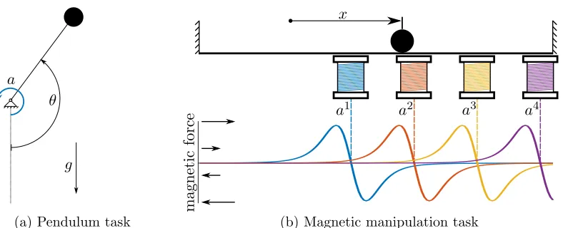
We perform our tests on two simulated control benchmarks: a pendulum swing-up task and a magnetic manipulation problem. Both were previously discussed by Alibekov et al. (2018). Although both represent dynamical systems with a two dimensional state-space, it will be shown in Section 6 that they are quite different when it comes to the optimal experience selection strategy. Here, a high level description of these benchmarks is presented, with the full mathematical description given in Appendix 9.3.

θ a

g

(a) Pendulum task

x

magnetic

force

a1 _a2 _a3 _a4

(b) Magnetic manipulation task

Figure 2: The two benchmark problems considered in this paper. In the pendulum task, an underactuated pendulum needs to be swung up and balanced in the upright position by controlling the torque applied by a motor. In the magnetic manipu-lation (magman) task, a steel ball (top) needs to be positioned by controlling the currents through four electromagnets. The magnetic forces exerted on the ball are shown at the bottom of the figure and can be seen to be a nonlinear function of the position. The forces scale linearly with the actionsa1_{, ..., a}4_{, which represent}

the squared currents through the magnets.

side is needed to build up momentum before swinging towards the upright position in the opposite direction. Once the pendulum is upright it needs to stabilize around this unstable equilibrium point. The state of the problem sE consists of normalized versions of the angle

θ and angular velocity ˙θ of the pendulum. The action space is a normalized version of the voltage applied to the motor that applies a torque to the pendulum. A reward is given at every time-step, based on the absolute distance of the state from the reference state of being upright with no rotational velocity.

The second benchmark is a magnetic manipulation (magman) task, in which the goal is to accurately position a steel ball on a 1-D track by dynamically changing a magnetic field. The relative magnitude and direction of the force that each magnet exerts on the ball is shown in Figure 2b. This force is linearly dependent on the actions, which represent the squared currents through the electromagnet coils. Normalized versions of the position x

and velocity ˙x form the state-space of the problem. A reward is given at every time-step, based on the absolute distance of the state from the reference state of having the ball at the fixed desired position.

In experiments where the buffer capacity C is limited, we take C = 104 experiences, unless stated otherwise. All our experiments have episodes which last four seconds. Unless stated otherwise, a sampling frequency of 50 Hz is used, which means the buffer can store 50 episodes of experience tupleshsi, ai, s0i, rii.

max-imum at episode 1, to a minmax-imum level from episode 500 onwards in all our experiments. At the minimum level, the amplitude of the exploration noise we add to the neural network policy is 10% of the amplitude at episode 1. Details of the exploration strategies used are given in Appendix 9.3.

5. Performance Measures and Experience Selection Notation

This section introduces the performance measures used and the notation used to distinguish between the experience selection strategies.

5.1 Performance Measures

When we investigate the performance of the learning methods in Sections 6 and 8, we are interested in the effect that these methods might have on three aspects of the learning performance: the learning stability, the maximum controller performance and the learning speed. We define performance metrics for these aspects, related to the normalized mean reward per episodeµr. The normalization is performed such thatµr = 0 is the performance

achieved by a random controller, while µr = 1 is the performance of the off-line dynamic

programming method described in Appendix 9.3. This baseline method is, at least for the noise-free tests, proven to be close to optimal.

The first learning performance aspect we consider is thestabilityof the learning process. As we have discussed in previous work (de Bruin et al., 2015, 2016a), even when a good pol-icy has already been learned, the learning process can become unstable and the performance can drop significantly when the properties of the training data change. We investigate to what extent different experience replay methods can help prevent this instability. We use the mean of µr over the last 100 episodes of each learning run, where the learning runs

should have converged to good behavior already, as a measure of learning stability. We denote this measure byµfinal_r .

Although changing the data distribution might help stability, it could at the same time prevent us from accurately approximating the true optimal policy. Therefore we also report themaximum performance achieved per learning trial µmax_r .

Finally, we want to know the effects of the experience selection methods on thelearning speed. We therefore report the number of episodes before the learning method achieves a normalized mean reward per episode of µr = 0.8 and denote this by Rise-time 0.8.

For these performance metrics we report the means and the 95% confidence bounds of those means over 50 trials for each experiment. The confidence bounds are based on bootstrapping (Efron, 1992).

5.2 Experience Selection Strategy Notation

Notation Proxy Explanation

FIFO age The oldest experiences are overwritten with new ones.

FULL DB - The buffer capacityC is chosen to be large enough to retain all experiences.

Table 1: Commonly used experience retention strategies for deep reinforcement learning.

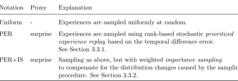
Notation Proxy Explanation

Uniform - Experiences are sampled uniformly at random.

PER surprise Experiences are sampled using rank-based stochasticprioritized experience replay based on the temporal difference error. See Section 3.3.1.

PER+IS surprise Sampling as above, but with weightedimportance sampling

to compensate for the distribution changes caused by the sampling procedure. See Section 3.3.2.

Table 2: Experience sampling strategies from the literature.

and sampling strategies commonly used in deep RL that were introduced in Section 3.3 are given in Tables 1 and 2 respectively. The abbreviations used for the new or uncommonly used methods introduced in Section 7 are given there, in Tables 4 and 5.

6. Analysis of Experience Utility

As previously noted by Schaul et al. (2016); Narasimhan et al. (2015); Pieters and Wiering (2016) and de Bruin et al. (2016a, 2015), when using experience replay, the criterion that determines which experiences are used to train the reinforcement learning agent can have a large impact on the performance of the method. The aim of this section is to investigate what makes an experience useful and how this usefulness depends on several identifiable characteristics of the control problem at hand.

In the following sections, we mention only some relevant aspects of our implementation of the deep reinforcement-learning methods, with more details given in Appendix 9.3.

6.1 The Limitations of a Single Proxy

0 500 1000 1500

Episode 0.60

0.65 0.70 0.75 0.80 0.85 0.90 0.95 1.00

µr

Pendulum swingup

selection FULL DB[PER]

FIFO[Uniform]

0 500 1000 1500

Episode

µr

Magman

selection FULL DB[PER]

FIFO[Uniform]

Figure 3: Comparison of the state-of-the-art (FULL DB[PER]) and the default method (FIFO[Uniform]) for experience selection on our two benchmark problems.

The first experience selection strategy tested is FIFO[Uniform]: overwriting the oldest experiences when the buffer is full and sampling uniformly at random from the buffer. We compare this strategy to the state-of-the-art prioritized experience replay method FULL DB[PER] by Schaul et al. (2016). Here, the buffer capacity C is chosen such that all experiences are retained during the entire learning run (C = N = 4×105 for this test).1 The sampling strategy is the rank-based stochastic prioritized experience replay strategy as described in Section 3.3. The results of the experiments are shown in Figure 3.

Figure 3 shows that FULL DB[PER] method, which samples training batches based on the temporal difference error from a buffer that is large enough to contain all previous experiences, works well for the pendulum swing-up task. The method very reliably finds a near optimal policy. The FIFO[Uniform] method, which keeps only the experiences from the last 50 episodes in memory, performs much worse. As we reported previously (de Bruin et al., 2016a), the performance degrades over time as the amount of exploration is reduced and the experiences in the buffer fail to cover the state-action space sufficiently.

If we look at the result on the magman benchmark in Figure 3, the situation is reversed. Compared to simply sampling uniformly from the most recent experiences, sampling from all previous experiences according to their temporal difference error limits the final perfor-mance significantly. As shown in Appendix 9.3, this is not simply a matter of the function approximator capacity, as even much larger networks trained on all available data are out-performed by small networks trained on only recent data. When choosing an experience selection strategy for a reinforcement learning task, it seems therefore important to have some insights into how the characteristics of the task determine the need for specific kinds of experiences during training. We will investigate some of these characteristics below.

6.2 Generalizability and Sample Diversity

One important aspect of the problem, which at least partly explains the differences in performance for the two methods on the two benchmarks in Figure 3, is the complexity of generalizing the value function and policy across the state and action spaces.

For the pendulum task, learning actor and critic functions that generalize across the entire state and action spaces will be relatively simple as a sufficiently deep neural network can efficiently exploit the symmetry in the value and policy functions (Montufar et al., 2014). Figure 4b shows the learned policy after 100 episodes for a learning run with FIFO[Uniform] experience selection. Due to the thorough initial exploration, the experiences in the buffer cover much of the state-action space. As a result, a policy has been learned that is capable of swinging the pendulum up and stabilizing it in both the clockwise and anticlockwise directions, although the current policy favors one direction over the other.

For the next 300 episodes this favored direction does not change and as the amount of exploration is decayed, the experiences in the buffer become less diverse and more centered around this favored trajectory through the state-action space. Even though the information on how to further improve the policy becomes increasingly local, the updates to the network parameters can cause the policy to be changed over the whole state space, as neural networks are global function approximators. This can be seen from Figure 4d, where the updates that further refine the policy for swinging up in the currently preferred direction have removed the previously obtained skill of swinging up in the opposite direction. The policy has suffered fromcatastrophic forgetting (Goodfellow et al., 2013) and has over-fitted to the currently preferred swing up direction.

For the pendulum swing up task, this over-fitting is particularly risky since the preferred swing up direction can and does change during learning, since both directions are equivalent with respect to the reward function. When this happens, the FIFO experience retention method can cause the data distribution in the buffer to change rapidly, which by itself can cause instability. In addition, the updates (4) and (6) now use the criticQ(s, a;θQ) function

in regions of the state-action space that it has not been trained on in a while, resulting in potentially bad gradients. Both of these factors might destabilize the learning process. This can be seen in Figure 4f where, after the preferred swing up direction has rapidly changed a few times, the learning process is destabilized and the policy has deteriorated to the point that it no longer accomplishes the balancing task. By keeping all experiences in memory and ensuring the critic errorδ stays low over the entire state-action space, the FULL DB[PER] method largely avoids these learning stability issues. We believe that this accounts for the much better performance for this benchmark shown in Figure 3.

-3 1 -1 velocity position 0 0 -2 -1 1 -1 0

(a) critic, episode 100

-1 1 -1 position velocity 0 0 -1 1 0 1

(b) actor, episode 100

-3 1 -1 position velocity 0 0 -2 1 -1 -1 0

(c) critic, episode 390

-1 1 -1 velocity position 0 0 1 -1 0 1

(d) actor, episode 390

-3 1 -1 position velocity 0 0 -2 -1 1 -1 0

(e) critic, episode 507

-1 1 -1 position velocity 0 0 1 -1 0 1

(f) actor, episode 507

Figure 4: The criticQ(s, π(s;θπ);θQ) and actorπ(s;θπ) functions trained on the pendulum

swing up task using FIFO[Uniform] experience selection. The surfaces represent the functions. The black dots show the trajectories through the state-action space resulting from deterministically following the current policy. The red and blue lines show respectively the positive and negative ‘forces’ that shape the surfaces caused by the experiences in the buffer: for the critic these areδ(s, a) (note a6=

π(s;θπ)). For the actor these forces represent∂Q(s, π(s;θπ);θQ)/∂a. Animations

0.0 0.2 0.4 0.6 0.8 1.0

µ

final r

buffer capacity =1·103 buffer capacity =1·104

P

endulum

swing-up

buffer capacity =1·105

0.0 0.05 0.1 0.2 0.5 1.0

synthetic sample fraction 0.0

0.2 0.4 0.6 0.8 1.0

µ

final r

0.0 0.05 0.1 0.2 0.5 1.0

synthetic sample fraction

0.0 0.05 0.1 0.2 0.5 1.0

synthetic sample fraction

Magman

Synthetic

none state action

Figure 5: The effect on the mean performance during the last 100 episodes of the learning runsµfinal_r of the FIFO[Uniform] method when changing a fraction of the observed experiences with synthetic experiences, for different buffer sizes.

6.2.1 Buffer Size and Synthetic Sample Fraction

To test the hypothesis that the differences in performance observed in Figure 3 revolve around sample diversity, we will artificially alter the sample diversity and investigate how this affects the reinforcement learning performance. We will do so by performing the fol-lowing experiment. We use the plain FIFO[Uniform] method as a baseline. However, with a certain probability we make a change to an experience hsi, ai, s0i, rii before it is written

to the buffer. We change either the state si or the action ai. The changed states and

actions are sampled uniformly at random from the state and action spaces. When the state is re-sampled the action is recalculated as the policy action for the new state including exploration. In both cases, the next state and reward are recalculated to complete the altered experience. To calculate the next state and reward, we use the real system model. This is not possible for most practical problems; it serves here merely to gain a better understanding of the need for sample diversity.

120 130 140 150 160

Rise-time

0.8

[episo

des]

buffer capacity =1·103 buffer capacity =1·104

P

endulum

swing-up

buffer capacity =1·105

0.0 0.05 0.1 0.2 0.5 1.0 synthetic sample fraction 200

400 600 800

Rise-time

0.8

[episo

des]

0.0 0.05 0.1 0.2 0.5 1.0 synthetic sample fraction

0.0 0.05 0.1 0.2 0.5 1.0 synthetic sample fraction

Magman

Synthetic none state action

(a) Effect on the number of episodes needed to reachµr= 0.8.

0.94 0.96 0.98

µ

max r

buffer capacity =1·103 buffer capacity =1·104

P

endulum

swing-up

buffer capacity =1·105

0.0 0.05 0.1 0.2 0.5 1.0 synthetic sample fraction 0.85

0.90 0.95 1.00

µ

max r

0.0 0.05 0.1 0.2 0.5 1.0 synthetic sample fraction

0.0 0.05 0.1 0.2 0.5 1.0 synthetic sample fraction

Magman

Synthetic none state action

(b) Effect on the number of maximum controller performance obtained per learning run.

For the magman benchmark, as expected, having more diverse states reduces the per-formance significantly. Having a carefully chosen fraction of more diverse actions in the original states can however improve the stability and learning speed slightly. This can be explained from the fact that even though the effects of the actions are strongly nonlinear in the state-space, they are linear in the action space. Generalizing across the action space might thus be more straightforward and it is helped by having the training data spread out over this domain.

6.3 Reinforcement-Learning Algorithm

The need for experience diversity also depends on the algorithm that is used to learn from those experiences. In the rest of this work we exclusively consider the DDPG actor-critic algorithm, as the explicitly parameterized policy enables continuous actions, which makes it especially suitable for control. An alternative to using continuous actions is to discretize the action space. In this subsection, we compare the need for diverse data of the actor-critic DDPG algorithm (Lillicrap et al., 2016; Silver et al., 2014) to that of the closely related critic-only DQN algorithm (Mnih et al., 2015). The experiments are performed on the pendulum benchmark, where the one dimensional action is divided uniformly into 15 discrete actions. Results for the magman benchmark are omitted as the four dimensional action space makes discretization impractical.

For the actor-critic scheme to work, the critic needs to learn a general dependency of the Q-values on the states and actions. For the DQN critic, this is not the case as the Q-values for different actions are separate. Although the processing of the inputs is shared, the algorithm can learn at least partially independent value predictions for the different

0.0 0.05 0.1 0.25 0.5

synthetic sample fraction 0.2

0.4 0.6 0.8 1.0

µ

final r

DDPG (state) DDPG (action) DQN (state) DQN (action)

(a) Effect on the mean performance during the last 100 episodes of the learning runsµfinal_r .

0.0 0.05 0.1 0.25 0.5

synthetic sample fraction 0

100 200 300 400 500

Rise-time

0.8

[episo

d

es]

(b) Effect on the number of episodes needed to reachµr= 0.8.

actions. These functions additionally do not need to be correct, as long as the optimal action in a state has a higher value than the sub-optimal actions.

These effects can be seen in Figure 7. The DDPG algorithm can make more efficient use of the state-action space samples by learning a single value prediction, resulting in significantly faster learning than the DQN algorithm. The DDPG algorithm additionally benefits from more diverse samples, with the performance improving for higher fractions of randomly sampled states or actions. The DQN algorithm conversely seems to suffer from a more uniform sampling of the state-action space. This could be because it is now tasked with learning accurate mappings from the states to the state-action values for all actions. While doing so might not help to improve the predictions in the relevant parts of the state-action space, it could increase the time required to learn the function and limit the function approximation capacity available for those parts of the state-space where the values need to be accurate. Note again that learning precise Q-values for all actions over the whole state-space is not needed, as long as the optimal action has the largest Q-value. Due to the better scalability of policy-gradient methods in continuous control settings, we exclusively consider the DDPG algorithm in the remainder of this work.

6.3.1 Sample Age

In the model-free setting it is not possible to add synthetic experiences to the buffer. Instead, in Section 7 we will introduce ways to select real experiences that have desirable properties and should be remembered for a longer time and replayed more often. This will inevitably mean that some experiences are used more often than others, which could have detrimental effects such as that the learning agent could over-fit to those particular experiences.

0.0 0.01 0.1 1.0

synthetic sample refresh probability 0.0

0.2 0.4 0.6 0.8 1.0

µ

final r

Pendulum swing-up

0.0 0.01 0.1 1.0

synthetic sample refresh probability 0.0

0.2 0.4 0.6 0.8 1.0

Magman

Synthetic fraction state [0.1] state [0.5] action [0.1] action [0.5]

To investigate the effects of adding older experiences for diversity, we perform the fol-lowing experiment. As before, a FIFO buffer is used with a certain fraction of synthetic experiences. However, when a synthetic experience is about to be over-written, we only sample a new synthetic experience with a certain probability. Otherwise, the experience is left unchanged. The result of this experiment is shown in Figure 8. For the pendulum benchmark, old experiences only hurt when they were added to provide diversity in the action space in states that were visited by an older policy. For the magman benchmark the age of the synthetic experiences is not seen to affect the learning performance.

6.4 Sampling Frequency

An important property of control problems that can influence the need for experience diver-sity is the frequency at which the agent needs to produce control decisions. The sampling frequency of a task is something that is often considered a given property of the environment in reinforcement learning. For control tasks however, a sufficiently high sampling frequency can be crucial for the performance of the controller and for disturbance rejection (Franklin et al., 1998). At the same time, higher sampling frequencies can make reinforcement learn-ing more difficult as the effect of taklearn-ing an action for a slearn-ingle time-step diminishes for increasing sampling frequencies (Baird, 1994). Since the sampling rate can be an impor-tant hyperparameter to choose, we investigate whether changing it changes the diversity demands for the experiences to be replayed.

In Figure 9, the performance of the FIFO[Uniform] method is shown for different sam-pling frequencies, with and without synthetic samples. The first thing to note is that, as expected, low sampling frequencies limit the controller performance. Interestingly, much of the performance loss on the pendulum at low frequencies can be prevented through

in-10 25 50 100 150 200 Sampling frequency [Hz] 0.0 0.2 0.4 0.6 0.8 1.0 µ final r Pendulum swing-up

10 25 50 100 150 200 Sampling frequency [Hz]

Magman

Synthetic

none state [0.5] action [0.5]

(a) Effect on the mean performance during the last 100 episodes of the learning runsµfinal

r .

10 25 50 100 150 200 Sampling frequency [Hz] 0.3 0.4 0.5 0.6 0.7 0.8 0.9 1.0 µ max r Pendulum swing-up

10 25 50 100 150 200 Sampling frequency [Hz]

Magman

Synthetic

none state [0.5] action [0.5]

(b) Effect on maximum controller performance per episodeµmax

r .

0 500 1000 1500

Episode 0.0

0.2 0.4 0.6 0.8 1.0

µr

Pendulum swingup [100Hz]

synthetic samples none

none [DE]

action [0.5]

action [0.5] [DE]

0 500 1000 1500

Episode

µr

Magman [200Hz]

synthetic samples none

none [DE]

action [0.5]

action [0.5] [DE]

Figure 10: The effect of synthetic actions and stochastically preventing experiences from be-ing written to the buffer [DE] for the FIFO[Uniform] method on the benchmarks with increased sampling frequencies.

creased sample diversity. This indicates that on this benchmark most of the performance loss at the tested control frequencies stems from the learning process rather than the funda-mental control limitations. When increasing the sampling frequencies beyond our baseline frequency of 50Hz, sample diversity becomes more important for both stability and per-formance. For the pendulum swing-up it can be seen that as sampling frequency increases further, increased diversity in the state-space becomes more important. For the magman, adding synthetic action samples has clear benefits. This is very likely related to the idea that the effects of actions become harder to distinguish for higher sampling frequencies (Baird, 1994; de Bruin et al., 2016b).

There are several possible additional causes for the performance decrease at higher frequencies. The first is that by increasing the sampling frequency, we have increased the number of data points that are obtained and learned from per episode. Yet the amount of information that the data contains has not increased by the same amount. Since the buffer capacity is kept equal, the amount of information that the buffer contains has decreased and the learning rate has effectively increased. To compensate for these specific effects, experiments are performed in which samples are stochastically prevented from being written to the buffer with a probability proportional to the increase in sampling frequency. The results of these experiments are indicated with [DE] (dropped experiences) in Figure 10 and are indeed better, but still worse than the performance for lower sampling frequencies.

The second potential reason for the drop in performance is that we have changed the problem definition by changing the sampling frequency. This is because the forgetting factor

γ determines how far into the future we consider the effects of our actions according to:

0.0 0.01 0.02 0.05 noise amplitude

0.0 0.2 0.4 0.6 0.8 1.0

µ

final r

Pendulum swing-up

0.0 0.01 0.02 0.05

noise amplitude 0.0

0.2 0.4 0.6 0.8 1.0

Magman

Synthetic none state [0.5] action [0.5]

Figure 11: Experiments with altered experiences and sensor and actuator noise. Results are from the last 100 episodes of 50 learning runs. A description of the performance measures is given in Section 5.1.

whereTs is the sampling period in seconds andτγ is the lookahead horizon in seconds. To

keep the same lookahead horizon, we recalculate γ, which is 0.95 in our other experiments (Ts = 0.02), to be γpendulum = 0.9747 (Ts = 0.01) and γmagman = 0.9873 (Ts = 0.005). To

keep the scale of the Q functions the same, which prevents larger gradients, the rewards are scaled down. Correcting the lookahead horizon was found to hurt performance on both benchmarks. The likely cause of this is that higher values of γ increase the dependence on the biased estimation of Q over the unbiased immediate reward signal (see Equation (4)). This can cause instability (Fran¸cois-Lavet et al., 2015).

6.5 Noise

The final environment property that we consider is the presence of sensor and actuator noise. So far, the agent has perceived the (normalized) environment state exactly and its (de-normalized) chosen actions have been implemented without change. Now we consider Equations (1) and (2) with σs =σa ∈ {0,0.01,0.02,0.05}. The results of performing these

experiments are shown in Figure 11. The results indicate that the need for data diversity is not dependent on the presence of noise. However, in Section 8.3 it will be shown that the methods used to determine which experiences are usefulcan be affected by noise.

6.6 Summary

Property Effect Explanation

Benchmark Very high The need for diverse states and actions largely depends on the ease and importance of generalizing across the state-actions space, which is benchmark dependent.

RL algorithm Very high Generalizing across the action space is fundamental to actor-critic algorithms, but not to critic-only algorithms with discrete action spaces.

Sampling frequency High The stability of RL algorithms depends heavily on the sampling frequency. Experience diversity can help learning stability. Having diverse actions at higher frequencies might be crucial as the size of their effect on the observed returns diminishes.

Buffer size Medium Small buffers can lead to rapidly changing data distributions, which causes unstable learning. Large buffers have more inherent diversity.

Sample age Low Although retaining old samples could theoretically be problematic, these problems were not clearly observable in practice.

Noise None The presence of noise was not observed to influence the

need for experience diversity, although it can influence experience selection strategies, as will be shown in Section 8.3.

Table 3: The dependence of the need for diverse experiences on the investigated environ-ment and reinforceenviron-ment learning properties.

benefits of diversity, the next section will propose strategies to obtain diverse experiences in ways that are feasible on real problems.

7. New Experience-Selection Strategies

7.1 Experience Retention

Although we showed in Section 6.4 that high sampling rates might warrant dropping expe-riences, in general we assume that each new experience has at least some utility. Therefore, unless stated otherwise, we will always write newly obtained experiences to the buffer. When the buffer is full, this means that we need some metric that can be used to decide which experiences should be overwritten.

7.1.1 Experience Utility Proxies

A criterion used to manage the contents of an experience replay buffer should be cheap enough to calculate,2 should be a good proxy for the usefulness of the experiences and should not depend on the learning process in a way that would cause a feedback loop and possibly might destabilize that learning process. We consider three criteria for overwriting experiences.

Age: The default and simplest criterion is age. Since the policy is constantly changing and we are trying to learn its current effects, recent experiences might be more relevant than older ones. This (FIFO) criterion is computationally as cheap as it gets, since determining which experience to overwrite involves simply incrementing a buffer index. For smaller buffers, this does however make the buffer contents quite sensitive to the learning process, as a changing policy can quickly change the distribution of the experiences in the buffer. As seen in Figure 4, this can lead to instability.

Besides FIFO, we also consider reservoir sampling (Vitter, 1985). When the buffer is full, new experiences are added to it with a probability C/i where i is the index of the current experience. If the experience is written to the buffer, the experience it replaces is chosen uniformly at random. Note that this is the only retention strategy we consider that does not write all new experiences to the buffer. Reservoir sampling ensures that at every stage of learning, each experience observed so far has an equal probability of being in the buffer. As such, initial exploratory samples are kept in memory and the data distribution converges over time. These properties are shared with the FULL DB strategy, without needing the same amount of memory. The method might in some cases even improve the learning stability compared to using a full buffer, as the data distribution converges faster. However, when the buffer is too small this convergence can be premature, resulting in a buffer that does not adequately reflect the policy distribution. This can seriously compromise the learning performance.

Surprise: Another possible criterion is the unexpectedness of the experience, as measured by the temporal difference errorδ from (4). The success of the Prioritized Experience Replay (PER) method of Schaul et al. (2016) shows that this can be a good proxy for the utility of experiences. Since the values have to be calculated to update the critic, the computational cost is very small if we accept that the utility values might not be

current since they are only updated for experiences that are sampled. The criterion is however strongly linked with the learning process, as we are actively trying to minimize δ. This means that, when the critic is able to accurately predict the long term rewards of the policy in a certain region of the state-action space, these samples can be overwritten. If the predictions of the critic later become worse in this region, there is no way of getting these samples back. An additional problem might be that the error according to (4) will be caused partially by state and actuator noise. Keeping experiences for which the temporal difference error is high might therefore cause the samples saved in the buffer to be more noisy than necessary.

Exploration: We introduce a new criterion based on the observation that problems can occur when the amount of exploration is reduced. On physical systems that are susceptible to damage or wear, or for tasks where adequate performance is required even during training, exploration can be costly. This means that preventing the problems caused by insufficiently diverse experiences observed in Section 6 simply by sustained thorough exploration might not be an option. We therefore view the amount of exploration performed during an experience as a proxy for its usefulness. We take the 1-norm of the deviation from the policy action to be the usefulness metric. In our experiments on the small scale benchmarks we follow the original DDPG paper (Lillicrap et al., 2016) in using an Ornstein-Uhlenbeck noise process added to the output of the policy network. The details of the implementation are given in Appendix 9.3. In the experiments in Section 8.5 a copy of the policy network with noise added to the parameters is used to calculate the exploratory actions (Plappert et al., 2018).

For discrete actions, the cost of taking exploratory actions could be used as a measure of experience utility as well. The inverse of the probability of taking an action could be seen as a measure of the cost of the action. It could also be worth investigating the use of a low-pass filter, as a series of (semi)consecutive exploratory actions would be more likely to result in states that differ from the policy distribution in a meaningful way. These ideas are not tested here, as we only consider continuous actions in the remainder of this work.

Note that the size of the exploration signal is the deviation of the chosen action in a certain state from the policy action for that state. Since the policy evolves over time we could recalculate this measure of deviation from the policy actions per experience at a later time. Although we have investigated using this policy deviation proxy previously (de Bruin et al., 2016b), we found empirically that using the strength of the initial exploration yields better results. This can partly be explained by the fact that recalculating the policy deviation makes the proxy dependent on the learning process and partly by the fact that sequences with more exploration also result in different states being visited.

7.1.2 Stochastic Experience Retention Implementation

Notation Proxy Explanation

Expl(α) Exploration Experiences with the least exploration are stochastically overwritten with new ones.

TDE(α) Surprise Experiences with the smallest temporal difference error are stochastically overwritten with new ones.

Resv Age The buffer is overwritten such that each experience observed so far has an equal probability of being in the buffer.

Table 4: New and uncommon experience retention strategies considered in this work.

Notation Proxy Explanation

Uniform + FIS - Experiences are sampled uniformly at random,

FIS (Section 7.2) is used to account for the distribution changes caused by theretention policy.

PER+FIS Surprise Experiences are sampled using rank based stochastic prioritized experience replay based on the temporal difference error. Full importance sampling is used to account for the distribution changes caused by both the retention and sampling policies.

Table 5: New experience sampling strategies considered in this work.

Additionally, although the overwrite metric we choose might provide a decent proxy for the usefulness of experiences, we might still want to be able to scale the extent to which we base the contents of the buffer on this proxy. We therefore use the same stochastic rank-based selection criterion of (7) suggested by Schaul et al. (2016), but now to determine which experience in the buffer is overwritten by a new experience. We denote this as TDE(α) for the temporal difference-based retention strategy and Expl(α) for the exploration-based policy. Here, α is the parameter in (7) which determines how strongly the buffer contents will be based on the chosen utility proxy. A sensitivity analysis ofαfor both Expl and PER is given in Appendix 9.3. The notation used for the new experience retention strategies is given in Table 4.

7.2 Experience Sampling

reten-tion and experience sampling strategies interact. In this context we introduce a weighted importance sampling method that accounts for the full experience selection strategy.

Importance sampling according to (8) can be used when performing prioritized experi-ence replay from a buffer that contains samples with a distribution that is unbiased with respect to the environment dynamics. When this is not the case, we might need to com-pensate for the effects of changing the contents of the buffer, potentially in addition to the current change in the sampling probability. The contents of the buffer might be the result of many subsequent retention probability distributions. Instead of keeping track of all of these, we compensate for both the retention and sampling probabilities by using the number of times an experience in the buffer has actually been replayed. When replaying an experience i for the K-th time, we relate the importance-weight to the probability under uniform sampling from a FIFO buffer of sampling an experience X times, where X is at least K: Pr(X ≥ K|FIFO[Uniform]). We refer to this method as Full Importance Sampling (FIS) and calculate the weights according to :

ωFIS_i = 



Pr(X ≥K|FIFO[Uniform]) h

Pdnpe

j=1 Pr(X≥j|FIFO[Uniform]) i

/np 



β

.

Here, nis the lifetime of an experience for a FIFO retention strategy in the number of batch updates, which is the number of batch updates performed so far when the buffer is not yet full. The probability of sampling an experience during a batch update when sampling uniformly at random is denoted by p. Note that np is the expected number of replays per experience, which following Schaul et al. (2016) we take as 8 by choosing the number of batch updates per episode accordingly. As in Section 3.3.2 we use β to scale between not correcting for the changes and correcting fully. Since the probability of being sampled at leastK times is always smaller than one forK >0, we scale the weights such that the sum of the importance weights for the expectednpreplays under FIFO[Uniform] sampling is the same as when not using the importance weights (n·p·1). The probability of sampling an experience at leastK times under FIFO[Uniform] sampling is calculated using the binomial distribution:

Pr(X≥K|FIFO[Uniform]) = 1−

K

X

k=0

n k

pk(1−p)n−k.

Correcting fully (β= 1) for the changed distributions would make the updates as unbi-ased as those from the unbiunbi-ased FIFO uniform distribution (Needell et al., 2016). However, since the importance weights of experiences that are repeatedly sampled for stability will quickly go to zero, it might also undo the stabilizing effects that were the intended outcome of changing the distribution in the first place. Additionally, as discussed in Section 3.3.2, the FIFO Uniform distribution is not the only valid distribution. As demonstrated in Sec-tion 8.4, it is therefore important to determine whether compensating for the retenSec-tion strategy is necessary before doing so.

0.6 0.8 1.0

µfinalr

FIFO[Uniform] FIFO[PER] TDE(1.20)[Uniform]

TDE(1.20)[PER] Expl(1.20)[Uniform] Expl(1.20)[PER] Resv[Uniform] Resv[PER] FULL DB[Uniform]

FULL DB[PER]

selection

0 100 200

Rise-time 0.8 [episodes]

0.6 0.8 1.0

µmaxr

(a) Swing-up

0.6 0.8 1.0

µfinalr

FIFO[Uniform] FIFO[PER] TDE(1.20)[Uniform]

TDE(1.20)[PER] Expl(1.20)[Uniform] Expl(1.20)[PER] Resv[Uniform]

Resv[PER] FULL DB[Uniform]

FULL DB[PER]

selection

0 250 500

Rise-time 0.8 [episodes]

0.6 0.8 1.0

µmaxr

(b) Magman

Figure 12: Performance of the experience selection methods under the default conditions of moderate sampling frequencies and no state or actuator noise. A description of the performance measures is given in Section 5.1.

8. Experience Selection Results

Using the experience retention and sampling methods discussed in Section 7, we revisit the scenarios discussed in Section 6. We first focus on the methods without importance sampling, which we discuss separately in Section 8.4. Besides the tests on the benchmarks of Section 4, we also show results on six additional benchmarks in Section 8.5. There we also discuss how to choose the size of the experience buffer.

8.1 Basic Configuration

and buffer size that determines the performance. It is again clear that this choice here depends on the benchmark. On the pendulum benchmark, where storing all experiences works well, the Resv method works equally well while storing only 104 experiences, which equals 50 of the 3000 episodes. On the magman benchmark, using a small buffer with only recent experiences works better than any other method.

Sampling according to the temporal difference error can be seen to benefit primarily the learning speed on the pendulum. On the magman, PER only speeds up the learning process when sampling from recent experiences. When sampling from diverse experiences, PER will attempt to make the function approximation errors more even across the state-action space, which as discussed before, hurts performance on this benchmark.

8.2 Effect of the Sampling Frequency

For higher sampling frequencies, the performance of the different experience selection meth-ods is shown in Figure 13. We again see that higher sampling frequencies place different demands on the training data distribution. With the decreasing exploration, retaining the right experiences becomes important. This is most visible on the Magman benchmark where FIFO retention, which resulted in the best performance at the end of training for the base sampling frequency, now performs worst. Retaining all experiences works well on both benchmarks. When not all experiences can be retained, the reservoir retention method is still a good option here, with the exploration-based method a close second.

8.3 Sensor and Actuator Noise

We also test the performance of the methods in the presence of noise, similarly to Section 6.5. The main question here is how the noise might affect the methods that use the temporal difference error δ as the usefulness proxy. The concern is that these methods might favor noisy samples, since these samples might cause bigger errors. To test this we perform learning runs on the pendulum task while collecting statistics on all of the experiences in the mini-batches that are sampled for training. The mean absolute values of the noise in the experiences that are sampled are given in Table 6. It can be seen that the temporal difference error-based methods indeed promote noisy samples. The noise is highest for those dimensions that have the largest influence on the value ofQ.

0.0 0.5 1.0

µfinalr

FIFO[Uniform] TDE(1.20)[Uniform] Expl(1.20)[Uniform] Resv[Uniform] FULL DB[Uniform]

selection

0 100 200

Rise-time 0.8 [episodes]

0.0 0.5 1.0

µmaxr

(a) Swing-up [100 Hz]

0.0 0.5 1.0

µfinalr

FIFO[Uniform] TDE(1.20)[Uniform] Expl(1.20)[Uniform] Resv[Uniform] FULL DB[Uniform]

selection

0 250 500

Rise-time 0.8 [episodes]

0.0 0.5 1.0

µmaxr

(b) Magman [200 Hz]

Figure 13: Performance of the experience selection methods with increased sampling fre-quencies. Results are from 50 learning runs. A description of the performance measures is given in Section 5.1.

position velocity action

Expl(1.0)[Uniform] 1.584 ·10−2 1.582·10−2 1.594·10−2 Expl(1.0)[PER] 1.654 ·10−2 1.630·10−2 1.595·10−2 TDE(1.0)[Uniform] 1.713·10−2 1.627·10−2 1.598·10−2 TDE(1.0)[PER] 1.846·10−2 1.743·10−2 1.594·10−2

0.6 0.8 1.0

µfinalr

FIFO[Uniform] FIFO[PER] TDE(1.20)[Uniform]

TDE(1.20)[PER] Expl(1.20)[Uniform] Expl(1.20)[PER] Resv[Uniform] Resv[PER] FULL DB[Uniform]

FULL DB[PER]

selection

0 100 200

Rise-time 0.8 [episodes]

0.6 0.8 1.0

µmaxr

(a) Swing-up [σs=σa= 0.02]

0.6 0.8 1.0

µfinalr FIFO[Uniform]

FIFO[PER] TDE(1.20)[Uniform]

TDE(1.20)[PER] Expl(1.20)[Uniform] Expl(1.20)[PER] Resv[Uniform] Resv[PER] FULL DB[Uniform]

FULL DB[PER]

selection

0 250 500

Rise-time 0.8 [episodes]

0.6 0.8 1.0

µmaxr

(b) Magman [σs=σa = 0.02]

8.4 Importance Sampling

Finally, we investigate the different importance sampling strategies that were discussed in Sections 3.3.2 and 7.2. We do this by using the FIFO, TDE and Resv retention strategies as representative examples. We consider the benchmarks with noise, since as we discussed in Section 3.3.2, the stochasticity in the environment can make importance sampling more relevant. The results are shown in Figure 15. We discuss per retention strategy how the sample distribution is changed and whether the change introduces a bias that should be compensated for through importance sampling.

FIFO: This retention method results in an unbiased sample distribution. When combined with uniform sampling, there is no reason to compensate for the selection method. Doing so anyway (FIFO[Uniform + FIS]) results in downscaling the updates from experiences that happen to have been sampled more often than expected, effectively reducing the batch-size while not improving the distribution. The variance of the updates is therefore increased without reducing bias. This can be seen to hurt perfor-mance in Figure 15, especially on the swing-up task where sample diversity is most important. Using PER also hurts performance in the noisy setting as this sampling proceduredoes bias the sample distribution. Using importance sampling to compen-sate for just the sampling procedure (FIFO[PER+IS]) helps, but the resulting method is not clearly better than uniform sampling.

TDE: When the retention strategy is based on the temporal difference error, there is a reason to compensate for the bias in the sample distribution. It can be seen from Figure 15 however, that the full importance sampling scheme improves performance on the magman benchmark, but not on the swing-up task. The likely reason is again that importance sampling indiscriminately compensates for both the unwanted re-sampling of the environment dynamics and reward distributions as well as the beneficial re-sampling of the state-action space distribution. The detrimental effects of compensating for the latter seen to outweigh the beneficial effects of compensating for the former on this benchmark where state-action space diversity has been shown to be so crucial.

Resv: The reservoir retention method is not biased with respect to the reward function or the environment dynamics. Although the resulting distribution is strongly off-policy (assuming the policy has changed during learning), this does not present a problem for a deterministic policy gradient algorithm with Q-learning updates, other than that it might be harder to learn a function that generalizes to a larger part of the state space. When sampling uniformly, we do sample certain experiences, from early in the learning process, far more often than would be expected under a FIFO[Uniform] selection strategy. The FIS method compensates for this by weighing these experiences down, effectively reducing the size of both the buffer and the mini-batches. In Figure 15, this can be seen to severely hurt the performance on the swing-up problem, as well as the learning stability on the magman benchmark.