Scalable Interpretable Multi-Response Regression via SEED
Zemin Zheng [email protected]
School of Management and School of Data Science International Institute of Finance
University of Science and Technololgy of China Hefei, Anhui 230026, China
M. Taha Bahadori [email protected]
School of Computational Science and Engineering Georgia Institute of Technology
Atlanta, GA 30332, USA
Yan Liu [email protected]
Computer Science Department Viterbi School of Engineering University of Southern California Los Angeles, CA 90089, USA
Jinchi Lv [email protected]
Data Sciences and Operations Department Marshall School of Business
University of Southern California Los Angeles, CA 90089, USA
Editor:Xiaotong Shen
Abstract
Sparse reduced-rank regression is an important tool for uncovering meaningful dependence structure between large numbers of predictors and responses in many big data applications such as genome-wide association studies and social media analysis. Despite the recent theoretical and algorithmic advances, scalable estimation of sparse reduced-rank regression remains largely unexplored. In this paper, we suggest a scalable procedure called sequential estimation with eigen-decomposition (SEED) which needs only a single top-rsparse singu-lar value decomposition from a generalized eigenvalue problem to find the optimal low-rank and sparse matrix estimate. Our suggested method is not only scalable but also performs simultaneous dimensionality reduction and variable selection. Under some mild regularity conditions, we show that SEED enjoys nice sampling properties including consistency in estimation, rank selection, prediction, and model selection. Moreover, SEED employs only basic matrix operations that can be efficiently parallelized in high performance computing devices. Numerical studies on synthetic and real data sets show that SEED outperforms the state-of-the-art approaches for large-scale matrix estimation problem.
Keywords: reduced-rank regression, scalability, high dimensionality, greedy algorithm, sparse eigenvector estimation
c
1. Introduction
Identifying complex dependence structures among predictors and responses is an important problem in statistics and machine learning, since these structures reveal hidden domain knowledge about the data. For example, in bioinformatics, identifying gene regulatory net-works is crucial for understanding gene regulatory paths and gene functions, which helps disease prediction and diagnosis. Similarly, in social media analysis, inferring the influ-ence networks from user activities, that is,Diffusion Network Inference problem (Leskovec et al., 2008; Zhou et al., 2013; Embar et al., 2014) is an important problem and it has found applications in social media marketing (Gomez-Rodriguez et al., 2012) and crisis manage-ment (Starbird and Palen, 2012). In these big data applications, inferring the dependence structures is challenging since the responses and predictors may be related through a few latent pathways and/or associated through only a subset of responses and predictors. More-over, the curse of dimensionality and massive amounts of data, that is, scalability issues make the dependence structure discovery problem even harder to solve. To recover sparse response-predictor associations and latent predictors, regularization methods such as lasso (Tibshirani, 1996) and group lasso (Yuan and Lin, 2006), and reduced-rank regression ap-proaches (Izenman, 1975; Velu and Reinsel, 2013) have been proposed, respectively. Chen et al. (2012) and Chen and Chan (2015) have proposed sparse reduced-rank regression ap-proaches by combining the regularization and reduced-rank regression techniques to find the complex dependence structures between responses and predictors.
Sparse reduced-rank regression works by modeling the associations between the predictor and response variables via a sparse and low-rank representation of the coefficient matrix. It not only enhances the interpretability of the estimated matrix by eliminating irrelevant features (Chen et al., 2012), but also reduces the number of free parameters of the model and thus the number of observations required for desired estimation consistency (Yuan et al., 2007; Bunea et al., 2011; Cand`es and Plan, 2011; Negahban and Wainwright, 2011; Chen et al., 2013). Sparse reduced-rank regression has found applications in micro-array biclustering (Chen et al., 2012), subspace clustering (Wang et al., 2013), social network community discovery (Richard et al., 2012; Zhou et al., 2013), and motion segmentation (Feng et al., 2014). In these applications, joint sparsity and low-rankness has been used to enforce a clustered dependence structure among data points. In particular, the key idea is to estimate a similarity matrix among data points that is simultaneously sparse and low-rank and then permute the rows and columns of the matrix to yield approximately block-diagonal structures, which naturally lead to clustering of data points into several groups. Note that Chandrasekaran et al. (2010), Agarwal et al. (2012), and the references therein have considered estimating matrices with a low-rank plus sparse representation which is different from our work as we are interested in estimating a matrix that is jointly low-rank and sparse.
lasso (RCGL), was proposed which directly penalizes the rank and the number of nonzero rows of the parameter matrix. They showed oracle rates for the estimated matrix and also provided a practical algorithm which iteratively and jointly solves a L1-regularization and low-rank estimation problem. To further improve the estimation accuracy, Chen et al. (2012) borrowed ideas from adaptive Lasso (Zou, 2006) and proposed the iterative exclusive extraction algorithm (IEEA) which finds a locally optimal solution in the neighborhood of the initial value. They also showed model selection consistency and asymptotic normality results along with the improved empirical performance of IEEA on microarray biclustering analysis data.
All the above approaches for sparse reduced-rank regression achieve both desirable the-oretical properties and strong empirical results. However, they cannot scale to large matrix estimation problems in many big data applications. The ADMM algorithm of Richard et al. (2012) and Zhou et al. (2013) uses iterative singular value thresholding (Cai et al., 2010) for solving the jointL1and nuclear norm regularization. Iterative singular value thresholding is known to be computationally expensive since it performs a full singular value decomposition of the parameter matrix in each iteration. On the other hand, RCGL (Bunea et al., 2012) is computationally much faster than ADMM since it only performs top-r singular value de-composition for estimating a rank-rmatrix in each iteration. Despite a lower computational cost per iteration, it is unclear how many iterations RCGL needs for convergence. IEEA (Chen et al., 2012) performs nested loops of alternating L1-penalized regression for each singular vector which can be expensive, especially on parallel computing devices. The iter-ative nature of these three approaches makes them not scalable and renders them inefficient for large matrix estimation even on high performance computing devices.
To overcome the scalability issues of the previous approaches, we propose a simple and scalable sparse reduced-rank regression procedure called sequential estimation with eigen-decomposition (SEED). SEED is designed for high-performing computing platforms. It converts the sparse and low-rank regression problem to a sparse generalized eigenvalue problem and then solves the problem using the recent algorithms for sparse eigenvalue decomposition (Cai et al., 2013; Ma, 2013; Yuan and Zhang, 2013). As a pure learning algorithm, SEED is expected to perform only a single top-r sparse eigenvalue decomposition for estimating a rank-r matrix, which makes it truly scalable and efficient for large matrix estimation problems.
Recently, Mishra et al. (2017) proposed the sequential co-sparse factor regression in a similar sparse and low-rank model setting, where a unit rank sparse coefficient matrix was recovered at each step such that both the left and the right singular vectors could be estimated with co-sparse pattern (an earlier version of the current paper was cited in theirs). Compared with their method, our approach separates the estimation of the singular vectors at each step with the left ones obtained through a generalized sparse eigenvalue problem and the right ones recovered directly based on the left ones. Moreover, we provide comprehensive theoretical properties to justify the validity of sequential estimation for sparse and low-rank coefficient matrices in high dimensions.
The rest of this paper is organized as follows. Section 2 introduces our SEED method. We discuss the implementation details of SEED in Section 3 and present its asymptotic properties in Section 4. We demonstrate the advantages of SEED on both synthetic and real data sets in Section 5, and in Section 6 we discuss some extensions of our SEED method. The proofs of some main results are relegated to the Appendix. Additional technical details are provided in the Supplementary Material.
2. Sequential Estimation with Eigen-Decomposition
We will first introduce the model setup and then the proposed methodology.
2.1. Model and Problem Formulation
Denote by{(xi,yi)}n
i=1nobservations in the fixed design setting, wherexi ∈Rpandyi ∈Rq represent the ith predictor and the corresponding response vectors, respectively. Given a predictor vectorx, the corresponding response vectory is drawn from the following model
y=C∗Tx+ε,
where the noise vectorε∼ N(0,Σ) is aq-dimensional multivariate Gaussian random vector with mean zero and covariance matrix Σ, and C∗ ∈ Rp×q is the regression coefficient
matrix.1 We can rewrite the model in the matrix form as follows
Y=XC∗+E, (1)
where Y= [y1, . . . ,yn]T,X = [x1, . . . ,xn]T, andE = [ε1, . . . ,εn]T denote the matrices of
stacked response, predictor and noise vectors, respectively.
Let P=n−1XTX be the Gram matrix of the predictors. We consider model (1) from a latent factor point of view, where the true regression coefficient matrix C∗ is jointly low-rank and sparse, similar to Bunea et al. (2012) and Chen et al. (2012). In particular, rank(C∗) =r∗ with the matrix rankr∗ min(p, q). Without loss of generality, we assume that rank(XC∗) = rank(C∗) since if rank(XC∗)<rank(C∗), the redundant part ofC∗ can be removed such that it reflects the true number of latent factors. Then C∗ will have the following decomposition
C∗ =
r∗
X
k=1
u∗kv∗Tk =
r∗
X
k=1
C∗k, (2)
where the left singular vectorsu∗k∈RpareP-orthogonal with unit length, that is,u∗T
k Pu∗k0 =
0 if k6=k0 and kuk∗k2 = 1, while the right singular vectorsv∗k∈Rq are orthogonal, that is, v∗Tk v∗k0 = 0 for k6=k0, and C∗k is the layer kunit rank matrix of C∗. The singular vectors
are sorted by the magnitudes of the singular valuesσk= √1nqkXC∗kkF in descending order,
consistent with their contributions to the prediction ofY.
We consider the left singular vectors (both the population and estimated ones) in the constraint spaceu ⊥Ker(P), where Ker(P) denotes the null space of P, to guarantee the model identifiability. Otherwise, u would contain certain component eu such that Xue = 0,
which does not contribute to the prediction ofY. It is worth noticing that the decomposition in the form of C∗ =Pr∗
k=1u∗kv∗Tk is not unique without orthogonality constraints and the
entrywise sparsity in the singular vectors is not invariant to rotations. The decomposition in (2) is a special one since theP-orthogonality of u∗k arises naturally from the power method and leads to a latent factor analysis interpretation of the reduced rank estimation in which the latent factors Xu∗k are uncorrelated. Moreover, decomposition (2) coincides with the singular value decomposition of XC∗ except for different scalings on the singular vectors. We defer the discussion on the identifiability of decomposition (2) (existence and uniqueness up to simultaneous sign changes ofu∗k and v∗k) to Supplementary Material.
The aforementioned modeling of the regression coefficient matrix gives a latent factor model withr∗latent factors, whereXu∗kis thekth latent factor andv∗kdescribes the impacts of the kth factor on the response variables. As illustrated in Yuan et al. (2007), the low-rankness of C∗ renders dimension reduction such that all responses can be predicted by a relatively small set of common factors. Furthermore, the left singular vectorsu∗kare assumed to be sparse, yielding the necessity of predictor selection. Similar sparsity assumptions were made in Bunea et al. (2012) and Chen et al. (2012) to enhance model interpretability by removing irrelevant features in high dimensions. Specifically, Chen et al. (2012) assumed that both the left and right singular vectors are sparse while Bunea et al. (2012) imposed restriction on the number of nonzero rows of the regression coefficient matrix. In this paper, we are interested in two cases: (i) when the right singular vectors are not required to be sparse and (ii) when it is desirable to have sparse right singular vectors, which entails the response selection. We will show that both cases are efficiently accommodated by our procedure.
Our goal is to accurately estimate the singular vectors u∗k and v∗k, and the true rank r∗ such that we can recover the latent factors, their impacts, and the underlying number of latent factors as well as the significant predictors. As a singular vector can have two opposite directions, we always assume that the estimated left singular vector takes the correct one, that is, the angles between estimated and population left singular vectors are no more than a right angle. Once the estimated rank and singular vectors are obtained, the estimateCb of
2.2. Description of SEED
The following proposition provides us insight into estimating the top-r∗ left and right sin-gular vectors ofC∗.
Proposition 1 Consider the noiseless case Y∗ =XC∗ with C∗ =Pr∗
k=1u
∗ kv
∗T
k defined in
(2). Then u∗1, . . . ,u∗r∗ are the r∗ non-degenerate left singular vectors of C∗ if and only if
they are eigenvectors of the following generalized eigenvalue problem
XTY∗Y∗TXu=λXTXu (3)
with respect to the nonzero eigenvalues λ1,· · · , λr∗, where λk = nqσ2
k is the kth largest
eigenvalue of Y∗Y∗T with σk =kXC∗kkF/
√
nq defined in Section 2.1. Furthermore, given the left singular vector u∗k, the corresponding right singular vector vk∗ can be written as
v∗k= 1
u∗Tk XTXu∗kY ∗TXu∗
k. (4)
Proposition 1 shows that the problem of estimating the singular vectors can be trans-formed into the generalized eigenvalue problem in (3), thanks to theP-orthogonality of the left singular vectors. It motivates us to estimate the left singular vectors in the noisy case
Y=XC∗+E by solving the following generalized eigenvalue problem
XTYYTXu=λXTXu. (5)
The estimation consistency can be guaranteed by the matrix perturbation theory (see Sec-tion 4 for details). On the other hand, it is not difficult to see that the eigenvectors with respect to different eigenvalues of problem (5) are P-orthogonal, which further gives the orthogonality of the right singular vectors estimated according to (4). It implies that the right and left singular vectors obtained by solving the generalized eigenvalue problem will automatically be orthogonal andP-orthogonal, respectively.
Related results of principal component analysis in low dimensions can be found in Baldi and Hornik (1989), Diamantaras and Kung (1996), and De La Torre and Black (2003). Note that in the high-dimensional setting, the regime of interest for this paper, the Gram matrix
P can not be invertible and the generalized eigenvalue problem is potentially challenging to solve. We will address the implementation challenges in Section 3.
Based on Proposition 1, our proposed procedure SEED performs a two-step estimation for the regression coefficient matrix. It first solves the generalized eigenvalue problem (5) to obtain the estimated left singular vectorsub1, . . . ,urb with unit length and then finds the
estimated right singular vectors bv1, . . . ,vbr according to (4) as follows
b
vk =
1
b
uTkXTXubk
YTXbuk. (6)
The maximum rank r depends on the magnitude of the estimated singular value σbk =
kXCkb kF/
√
nq with Ckb =ukb bvkT (whether it is larger than a thresholdµ) and the optimal
Algorithm 1:SEED
Input: (1) DataY∈Rn×q and X∈Rn×p (2) Termination accuracyµand sparsity
parameterθ
1 Compute matrices: P← n1XTX, R← n1YTX, Q← 1qR>R
2 k←1
3 repeat
4 (ubk,σbk)←kth θ-sparse eigenvector and eigenvalue of Qu=λPu
5 if bσk> µ then
6 bvk← 1
b
u>
kPbuk
Rubk #Optional thresholding of vbk for sparsity
7 Cbk ←ubkbvk>
8 k←k+ 1
9 end
10 until bσk < µ
11 tune the optimal rank br 12 return Cb =
Pbr k=1Cbk
The details of the procedure are provided in Algorithm 1. To achieve a sparse solution, we need to find the rank-r sparse matrix via a sparse eigenvalue decomposition procedure in Line 4 of Algorithm 1. This can be done in a sequential way and practical methods will be provided in Section 3. The practical methods need a sparsity parameter θ, such as a threshold (Ma, 2013) or a sparsity size (Yuan and Zhang, 2013). We will show in Section 5 that SEED is robust to the choices of parametersθ andµ. If the right singular vectors are also required to be sparse, we perform a simple element-wise thresholding on vkb after we
obtain it in Line 6.
3. Scalable Implementation of SEED
Algorithm 1 requires a sparse solution of (5) which is a generalized eigenvalue problem with a rank deficient matrixP. In this section, we propose two different procedures to solve (5) and study multiple practical aspects of SEED.
3.1. Fast Approach
The bottleneck in speeding up Algorithm 1 is Line 4 where we need to solve a sparse generalized eigenvalue problem. To overcome this bottleneck, we propose a new solution to estimating the left singular vectors by rewriting equation (5) as
XT(YYT −λI)Xu=0.
(1) λ←λmax(YYT).
(2) ub1 ←sparse eigenvector relative to the zero eigenvalue ofX
TYYTX−λXTX.
Based onbu1, the corresponding right singular vectorvb1 and the unit rank matrixCb1will be
obtained. To continue, we compute the residual Yk=Y−X
Pk−1
j=1Cjb in thekth step and
replace Y with Yk in the above two-step procedure to obtain the kth left singular vector
b
uk. Overall, the first step requires calculation of the top-r eigenvalues for an n×nmatrix
(or q×q ifq < n) while the second step finds the corresponding eigenvectors by solving a regular sparse eigenvalue problem.
The above procedure significantly accelerates the speed of SEED as it converts a de-generate sparse generalized eigenvalue problem to two simpler regular sparse eigenvalue problems. Existing procedures such as the iterative thresholding method (Ma, 2013) can be used to compute both eigenvalue problems efficiently. Generally speaking, SEED will be extremely efficient in applications with low rank structure such as image processing as it stops early after achieving a few important signals. Moreover, the speed of SEED can be greatly enhanced by parallel implementation on high performance computing devices such as GPU, due to the fact that it employs only basic matrix operations.
3.2. Alternative with Enhanced Stability
In cases where the perturbation can be large, for numerical stability purposes, we can also solve (5) by the following modified problem with a very small positiveρ:
XTYYTXu=λ(XTX+ρI)u. (7)
Note that XTX+ρI is invertible since the eigenvalues of XTX are nonnegative. Denote by Xe ∈ Rp×p the modified predictor matrix such that Xe
T
e
X = XTX+ρI, which can be obtained via the Cholesky decomposition, and Ye = (Xe
T
)−1XTY the modified response matrix. Then the above equation (7) can be rewritten as
e
XTYeYe
T
e
Xu=λXe
T
e
Xu, (8)
which adopts the same form as (5).
A computationally efficient technique for solving equation (8) is to solve the sparse
eigenvalue problem Pe
−1
e
Qu=λu, where the modified Gram matrix Pe =n−1Xe
T
e
X and Qe
is defined accordingly as in Algorithm 1. We can computePe
−1
by the Sherman-Morrison-Woodbury formula as follows:
(ρIp+XTX)−1 =
1 ρIp−
1 ρ2X
T(I n+
1 ρXX
T)−1X.
The above equation requires inversion of ann×nmatrix instead of a p×p matrix, which is significantly faster in the high-dimensional setting when pn.
Remark. The formulation of Xe and Ye can be regarded as a generalization of the
of kY∗−XCk2F, we can enhance the stability by adding a small Frobenius norm regular-ization as follows:
e
C= argminCnkY−XCkF2 +ρkCk2Fo, where the Frobenius norm is defined askCk2
F =
P
i,jC2i,j for any matrixC. After
complet-ing the squares, we get
e
C= argminCnkYe −XCe k2F o
,
which means that Xe and Ye are the corresponding predictor and response matrices that
take into account the shrinkage effects (James and Stein, 1961; Zheng et al., 2014).
3.3. Practical Aspects
Now we analyze several practical aspects of SEED as follows.
Refitting. In Algorithm 1, a refitting can be performed during the eigenvalue decompo-sition in Line 4 to enhance the stability. The refitting procedure is as follows. In the kth step, we perform the top-ksingular value decomposition Cb =USVb T forCb =
Pk
j=1Cbj and
refit the solution by finding Se = argminS
Y−XUSVT
2
F. The estimate with refitting
is defined as Ce = USVe T. In practice, we find this approach more stable and report the
results based on this variation of SEED in numerical studies.
Sparse eigenvector estimation. The previous approaches for solving the generalized eigenvalue decomposition problem indicate that we can solve the problem via regular sparse eigenvalue decomposition. This allows us to reuse the existing procedures for sparse eigen-value decomposition such as Cai et al. (2013), Ma (2013), Yuan and Zhang (2013), and Lei and Vu (2015) to solve the problem in (5). In numerical studies, we use the iterative thresholding method (Ma, 2013), which is detailed in Algorithm 2 for estimating the sparse eigenvector relative to the largest eigenvalue of a given sparse eigenvalue problemSu=λu
with sparsity parameter θ(threshold level).
It is worth pointing out that although sparse eigenvalue decomposition is a nonconvex problem, Ma (2013) proved that the sparse eigenvectors obtained by the iterative threshold-ing algorithm will converge to their population counterparts with asymptotic probability one within O(logn) iterations. The initial estimate ub(0) is generated from the diagonal thresholding sparse PCA algorithm proposed in Johnstone and Lu (2009), which is a reg-ular eigenvalue problem after constraining on the significant coordinates (variances). This iterative thresholding algorithm can also be applied to recover several sparse eigenvectors simultaneously.
Algorithm 2:Iterative thresholding
Input: MatrixS∈Rp×p, threshold levelθ, and initial estimate ub
(0) ∈
Rp.
1 k←1
2 repeat
3 Multiplication: t(k)= (tij(k)) =Sub(k−1) 4 Thresholding: bt
(k) = (bt
(k)
ij ) withbt
(k)
ij =t
(k)
ij 1(|tij|≥θ) 5 QR factorization: ub(k)R(k)=bt
(k)
with R(k)=kbt
(k) k2
6 k←k+ 1.
7 until convergence
8 return ub(k) at convergence
4. Asymptotic Properties of SEED
In this section, we will analyze the statistical properties of SEED. Define the maximum sparsity level of the left singular vectors as s∗ = maxrk∗=1ku∗kk0 p, which is assumed mainly for theoretical analysis (see Condition 1 below) and unknown in our practical im-plementation. We consider the estimated left singular vectors with the number of nonzero elements less than certain sparsity level s > s∗, that is, kbukk0 ≤s fork = 1,· · ·, r, where
r > r∗ is an upper bound of the estimated rank that can be controlled by the algorithm in practice. When the generalized eigenvalue problem (5) does not have ans-sparse solution, the estimated largest s-sparse eigenvalue can be reformulated as
b
λ= max
u6=0,kuk0≤s
uT(XTYYTX)u uT(XTX)u
due to the extremal property of eigenvalues, and the corresponding maximizer bu will be treated as the estimated left singular vector. Note that there is no sparsity constraint on either the population or the estimated right singular vectors sincev∗kcan be recovered from (4) based on accurate estimation of u∗k.
4.1. Technical Conditions
Here we list a few technical conditions and discuss their relevance in detail.
Condition 1 (Restricted Isometry) There exists a positive constant φs such that the
Gram matrix P satisfies
φs≤min
z∈Rp
k
Pzk2 kzk2
:kzk0≤2s
≤max
z∈Rp
k
Pzk2 kzk2
:kzk0≤2s
≤φ−s1
for some s > s∗.
Condition 2 (Minimum Singular Value Separation) The non-zero singular valuesσk
Condition 3 (Bounded Eigenvalues) The eigenvalues of the population covariance ma-trix of the noise vector ε satisfy 0 < γl2 ≤λj(Σ) ≤γu2 <∞ for j= 1, . . . , q, where γl and γu are positive constants with γu ≤cγσr∗ for some positive constant cγ.
Condition 4 (Minimum Signal Strength) There exists some positive constantδ ∈(0,1) such that the following lower bounds on the magnitudes of the non-zero elements ofu∗k and
v∗k hold for any 1≤k≤r∗
min
i∈supp(u∗
k)
|u∗i| ≥3Cu
r
s nlog
pq δ ,
min
i∈supp(v∗
k)
1
√
q|v ∗
i| ≥3Cv
r
s nlog
pq δ ,
where Cu and Cv are constants defined in Theorem 1.
Condition 1 imposes bounds on the 2s-sparse eigenvalues of P, which is weaker than the regular bounded eigenvalue assumption since the sparse eigenvalues do not grow as fast as the regular eigenvalues when the dimensionality p increases. As a typical condition in high dimensions, it restricts the correlations between small numbers of features and thus guarantees the identifiability of the true support. See, for instance, Cand`es and Tao (2005) and Zhang (2011) for more discussion on it.
Recall thatσkis thekth largest singular value ofXC∗/
√
nq. Condition 2 requires strict separation among the singular values such that the left singular vectors are distinguishable. For ease of presentation, we assumedσ to be a constant and indicate the roles ofdσ clearly
in the constants of the theoretical results. In fact, XC∗ adopts a spiked eigen-structure (Johnstone, 2001; Shen et al., 2016) with the spiked singular values allowed to diverge at the rate of √nq. This rate is reasonable for an n by q matrix as we do not impose any sparsity on the columns ofC∗.
The elements of the unobserved noise vector ε were assumed to be independent and identically distributed (i.i.d.) in Bunea et al. (2012). We relax it a bit in Condition 3 by imposing bounded eigenvalues for the noise covariance matrix for recovering the true rank in Theorem 2. Our technical argument still applies when either γl →0 or γu → ∞ as long
as their rates of convergence can be controlled within certain magnitudes.
The two inequalities in Condition 4 are imposed for the model selection consistency of the predictors and responses, respectively. The magnitude of the minimum signal strength is Opslog(pq)/n, which is relatively mild as it converges to zero in our setting. Since
u∗k is assumed to have unit length, the singular values of C∗ are absorbed into v∗k in view of decomposition (2) so that there is an extra scaling factor √1
q in the second inequality.
4.2. Main Results
Denote by P2 = maxpj=1Pjj and γ2 = maxqj=1Σjj the maximum diagonal components of the Gram matrix and noise covariance matrix, respectively. Without loss of generality, we assume that V = maxrk∗=1√1
qkv ∗
kk2 is finite for theq-dimensional vectors v∗k. Moreover, it
is clear that under Conditions 1 and 3, P and γ are also finite constants. The estimated regression coefficient matrix is given byCb =
Pr˜
by information criterion (9) andCbk=ubkvbTk. The following theorem bounds the estimation
errors of SEED with the estimated left singular vectors buk taking the correct signs as
discussed before.
Theorem 1 (Consistency of Estimation and Prediction) Suppose that Conditions 1 and 2 hold, γ is finite, and slog(pq) = o(n), then with probability at least 1−δ for any
δ∈(0,1)and uniformly over k= 1, . . . , r∗, we have
kubk−u∗kk2 ≤Cu
r
s nlog
pq δ +o
r s nlog pq δ , 1 √
qkvbk−v
∗
kk2 ≤Cv
r
s nlog
pq δ +o
r s nlog pq δ ,
kX(ubk√−u∗k)k2
n ≤ Cu √ φs r s nlog pq δ +o
r s nlog pq δ , 1 √
qkCbk−C ∗
kkF ≤(V Cu+Cv)
r s nlog pq δ +o r s nlog pq δ ,
kX(Ckb −C∗k)kF
√
nq ≤
(V C√u+Cv) φs r s nlog pq δ +o r s nlog pq δ ,
where the constants Cu = 4γP σ1 dσφ5s/2
and Cv = 2
√
2φ−s3/2(2V φ −1/2
s +σ1)Cu+ 2
√
2φ−s1γP. Theorem 1 is established based on the perturbation theory of sparse generalized eigen-value problem (Lemma 6). It shows that the uniform estimation error bounds for both top-r∗ singular vectors u∗k and √1
qv ∗ k, top-r
∗ latent factors √1
nXu ∗
k and unit rank matrices
1
√ qC
∗
k, and the uniform prediction error bounds of the top-r
∗ latent factors are all in the
same order of O
q s nlog pq δ
. The tail probabilityδ can decay to zero quickly asp and q
grow with rates such asδ∝(pq)−α for some positive constantα >1. This is due to the fact
that when δ∝(pq)−α, we haveqnslogpqδ →0 under the assumption thatslog(pq) =o(n). Furthermore, the estimation and prediction accuracy would then be within the rate of Opslog(pq)/n, where the factor log(pq) reflects the curse of dimensionality as there are pq parameters in total from the regression coefficient matrixC∗.
If the true rankr∗ can be correctly identified, it is not difficult to see that the estimation accuracy for √1
qC
∗ will be within the rate of O{p
r∗slog(pq)/n} (see Corollary 3 below),
which coincides with the minimax error bound for estimating the regression coefficient vector in the univariate response setting (Raskutti et al., 2011) with the dimensionality p and sparsity levelsreplaced by the overall dimensionalitypqand the product r∗s, respectively.
Similarly, with the true rank r∗, the normalized prediction error kX(Cb −C∗)kF/
√
nq
will be within the rate of O
np
r∗slog(pq)/n
o
zero asymptotically. Overall speaking, the prediction error bound in Bunea et al. (2012) was derived from the regularization framework, while the prediction accuracy of SEED is obtained from the matrix perturbation theory (Lemmas 5 and 6).
Based on the discussion before, a desirable statistical property of any low-rank estima-tion procedure is accurately recovering the true rank of the parameter matrix. Similar to Lasso, the nuclear norm regularization needs to be enhanced by techniques such as adaptive regularization to accurately recover the rank of the matrix (Bach, 2008; Chen et al., 2013). In contrast, we can directly control the rank of the solution in SEED by limiting the number of steps. In particular, we propose a GIC-type (Fan and Tang, 2013) information criterion that guarantees rank recovery by SEED when the optimal rank is tuned according to it.
Theorem 2 (Consistency of Rank Recovery) Suppose Conditions 1-3 hold,slog(pq) = o(n), r∗=o
1 √
(log logn)∨√s ·
h
n
log(pq)
i14
, and r=o
h
n slog(pq)
i14
. Define the following in-formation criterion
Cn=√nlogLn(Y,X,Cb) + rank(Cb) p
log(pq) log logn, (9)
where Ln(Y,X,C) = qn1 kY−XCk2F. Under the above information criterion, with
proba-bility at least 1−(pq)−α for some positive constant α >1 and sufficiently large n, SEED will select the true rank, that is, rank(Cb) = rank(C∗).
In the high-dimensional setting where the number of predictors can increase exponen-tially with the sample size, it is demonstrated in Fan and Tang (2013) that we need some power of the logarithmic factor of dimensionality (plog(pq) for our setting) in the model complexity penalty of the information criterion to consistently identify the true model, and the slow diverging rate log logn is set to prevent underfitting. The proof of Theorem 2 indeed shows that information criterion (9) will keep decreasing until the estimated rank reaches the true rankr∗, where in each step the amount of decrease in the objective function
Ln(Y,X,Cb) equals to the squared singular value obtained by solving the generalized
eigen-value problem (5). After reaching the true rank, the estimated singular eigen-value becomes small such that the model complexity penalty will overweight the decrease and then information criterion (9) would start increasing. Therefore, in the sequence of solutions generated by SEED, the estimate Cb with rank r∗ will be the minimizer of (9) such that the true rank
can be correctly identified.
As discussed before, correct identification of the true rank will yield the estimation accuracy of C∗ as well as the prediction accuracy of XC∗. Therefore, combined with Theorem 2, it is immediate that the results in Theorem 1 give the following corollary.
Corollary 3 (Consistency of Overall Estimation and Prediction) Given Conditions 1-3, slog(pq) = o(n), r∗ = o
1 √
(log logn)∨√s ·
h
n
log(pq)
i14
, and r = o
h
n slog(pq)
i14
for any constant α >0 and sufficiently large n, we have
1
√
qkCb −C ∗k
F ≤(1 +α)(V Cu+Cv)
r
r∗slog(pq) n
!
+o
r
r∗slog(pq) n
!
,
kX(Cb −C∗)kF
√
qn ≤
(1 +α)(V Cu+Cv)
√
φs
r
r∗slog(pq) n
!
+o
r
r∗slog(pq) n
!
.
Besides estimation consistency and rank recovery, SEED is also able to find the true support of the singular vectors. To achieve this goal, after selecting the optimal rank, we need to further refine the model selection procedure by performing a hard-thresholding. See, for example, Fan and Lv (2013) for applications of thresholding in high-dimensional sparse modeling. Specifically, denote by Tθ(z) the estimator after the hard-thresholding
operation on every element ofz= (z1,· · ·, zp)∈Rp such that
Tθ(zi) =
0 if|zi|< θ zi otherwise
, i= 1, . . . , p.
Based on the results of Theorems 1 and 2 and the signal strength assumption in Condition 4, we have the following properties for the estimator with a further thresholding.
Theorem 4 (Support Recovery of Singular Vectors) Given Conditions 1-4,slog(pq) =o(n), r∗ =o
1 √
(log logn)∨√s·
h
n
log(pq)
i1
4
, and r=o
h
n slog(pq)
i1
4
, for every pair of sin-gular vectors, (ubk,vbk), k= 1, . . . , r
∗, the following results hold.
a) If the threshold θ∈(54Tu,47Tu) withTu =Cu
q
s nlog
pq
δ, then with probability at least
1−δ, we have supp(Tθ(buk)) = supp(u
∗ k);
b) If the thresholdθ ∈(54Tv,47Tv) with Tv =Cv
q
qs n log
pq
δ, then with probability at least
1−δ, we have supp(Tθ(bvk)) = supp(v
∗ k).
Theorem 4 shows that both supports of the left and right singular vectors can be ac-curately recovered with properly chosen tuning parameter θ. Together with the correctly identified true rankr∗, the above results indeed yield consistent selection of both predictors and responses. In practice, this thresholdθcan be tuned by criteria such as cross-validation. Besides the statistical properties established before, the proposed procedure SEED en-joys great flexibility in the sense that it does not rely on exact eigenvalue decomposition and the perturbation errors in the generalized eigenvalue problem (5) will be linearly incor-porated into the estimated singular vectorsubk andvbk. Furthermore, our analysis does not
5. Numerical Studies
In this section, we conduct experiments on three data sets, including two simulation data sets (one for a medium-scale experiment and one for a large-scale experiment) and one application data set in social media analysis, to examine the empirical performance of SEED.
5.1. Simulation Studies
5.1.1. Simulation Example 1
We generate a medium-scale synthetic data set as follows: the predictorsx are drawn from a multivariate Gaussian distribution asx∼ N(0p×1,ΣX), whereΣX is thep×pcovariance matrix with auto-regressive structure, that is, ΣX,i,j = ρ|i−j| for some 0 < ρ < 1 which
will be specified later. The responses y are drawn according to conditional distribution
y|x ∼ N(C>x, γΣE) where the noise covariance matrix ΣE is also selected to have the autoregressive structure with ρ = 0.5 and we set γ = 0.3. We generate the parameter matrixCas follows: first we generate a block-sparse matrixCe with 5% non-zero elements.
Each non-zero element ofCe is drawn from aN(0,1). To achieve a low-rank structure, we
find the top-r singular value decomposition of Ce asCe =USVT, and then set the elements
of U and V whose magnitude is smaller than 0.01 to zero to obtain ¯U and ¯V. The final parameter matrix is obtained as C = ¯US¯V¯T where the first r diagonal elements of the diagonal matrix ¯S are set to 100,99, . . . ,101−r. Without loss of generality, we add a few vectors to the design matrix to ensure the orthogonality condition of Section 4.1. In all of the simulation experiments, we generate 100 data sets and report the mean and standard error of performance for different methods.
We compare the performance of SEED with two state-of-art methods: (1) RCGL (Bunea et al., 2012) and (2) Penalized regression with simultaneousL1 and nuclear-norm penaliza-tion. The optimization problem is solved by the popular alternating direction method of multipliers (Boyd et al., 2010) and we will refer to this baseline as the “ADMM” algorithm. For a fair comparison, all model parameters are set based on a separate validation set with sizenvalid = 500. To tune the parameters in SEED, we created a grid of sparsity thresholds
θ and for each value of θ, the validation errors were recorded while increasing the rank of the solution matrices. The robustness of sparsity thresholdθ and termination parameterµ will also be analyzed.
The quality of the estimatorCb is evaluated via four performance metrics listed as follows.
(1)Normalized Prediction Error defined as
Normalized Prediction Error = kYtest−XtestCbkF
kYtestkF .
(2)Normalized Parameter Estimation Error defined as
Normalized Parameter Estimation Error = kCb −CkF
kCkF ,
(3)Rank Recovery Error defined as
Rank Recovery Error =|rank(Cb)−rank(C)|.
Since the solution of the nuclear norm always leads to small non-zero singular values (which preventsCb from being low-rank), we threshold the singular values ofCb that are more than
100 times smaller than its largest singular value to have a fair comparison.
(4) Support Recovery AUC, that is, the area under the receiver operating characteristic (ROC) curve of comparing support of Cb with the ground truth, which is always between
0 and 1. It is computed by varying the decision threshold and obtaining the false positive and true positive curve. Then the area under the false positive and true positive curve is reported as AUC. The value of AUC indicates the probability that a procedure assigns a higher value to a randomly chosen non-zero element than a randomly chosen zero element (Hanley and McNeil, 1982). It is an appropriate metric for measuring support recovery accuracy because in sparse support recovery we have more zeros than non-zeros which inflates the result of the simple 0-1 accuracy measure. In contrast, AUC is more robust to imbalanced positive/negative prediction labels.
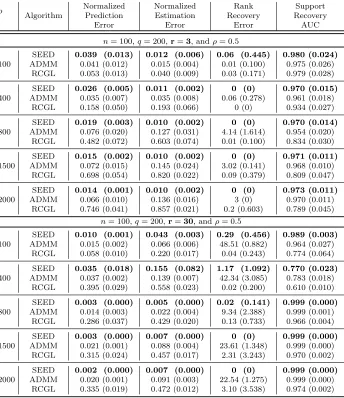
Table 1 shows the results of all algorithms on a variety of regimes by varying the dimen-sionalitypand the rankr. We can see that SEED is superior or comparable to the baseline algorithms across all four measures. As the results show and the theory predicts, in most high-dimensional cases, nuclear norm usually overestimates the true rank of the matrix. Furthermore, we find that the iterative SVD procedure in the RCGL algorithm often re-sults in significant underestimation of the true rank, when the true rank is large. Note that in addition to accuracy, SEED also significantly reduces the variance of the estimation.
Figure 1a shows the solution path for SEED on one example data set (p= 400,r = 5,q= 200, ρ= 0.5, andn= 100). The corresponding singular values are set to 30,27,24,21, and 18. In the horizontal axis, we show the termination parameterµnormalized bykYk2
F/(nq).
We can see that SEED can identify the correct rank with medium values of µ. Figure 1b shows the solution path for the top left singular vector u1 of C on an example data set (p = 200, q = 100, n= 50, ρ = 0.5, and r = 1). Both of the solution paths indicate that SEED is robust to the particular choice of parameters and in a large range of parameters SEED is able to successfully recover the true rank of the matrix and the support of the singular vectors.
5.1.2. Simulation Example 2
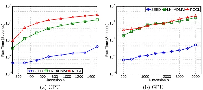
In order to study scalability of SEED, we conduct the experiments on two computing envi-ronment, including: (1) an off-the-shelf personal computer (PC) and (2) a graphics process-ing unit (GPU), to demonstrate the runtime efficiency and the parallelization capability of SEED.
p Normalized Normalized Rank Support
Algorithm Prediction Estimation Recovery Recovery
Error Error Error AUC
n= 100,q= 200,r=3, andρ= 0.5 100
SEED 0.039 (0.013) 0.012 (0.006) 0.06 (0.445) 0.980 (0.024)
ADMM 0.041 (0.012) 0.015 (0.004) 0.01 (0.100) 0.975 (0.026) RCGL 0.053 (0.013) 0.040 (0.009) 0.03 (0.171) 0.979 (0.028) 400
SEED 0.026 (0.005) 0.011 (0.002) 0 (0) 0.970 (0.015)
ADMM 0.035 (0.007) 0.035 (0.008) 0.06 (0.278) 0.961 (0.018) RCGL 0.158 (0.050) 0.193 (0.066) 0 (0) 0.934 (0.027) 800
SEED 0.019 (0.003) 0.010 (0.002) 0 (0) 0.970 (0.014)
ADMM 0.076 (0.020) 0.127 (0.031) 4.14 (1.614) 0.954 (0.020) RCGL 0.482 (0.072) 0.603 (0.074) 0.01 (0.100) 0.834 (0.030) 1500
SEED 0.015 (0.002) 0.010 (0.002) 0 (0) 0.971 (0.011)
ADMM 0.072 (0.015) 0.145 (0.024) 3.02 (0.141) 0.968 (0.010) RCGL 0.698 (0.054) 0.820 (0.022) 0.09 (0.379) 0.809 (0.047) 2000
SEED 0.014 (0.001) 0.010 (0.002) 0 (0) 0.973 (0.011)
ADMM 0.066 (0.010) 0.136 (0.016) 3 (0) 0.970 (0.011) RCGL 0.746 (0.041) 0.857 (0.021) 0.2 (0.603) 0.789 (0.045)
n= 100,q= 200,r=30, andρ= 0.5 100
SEED 0.010 (0.001) 0.043 (0.003) 0.29 (0.456) 0.989 (0.003)
ADMM 0.015 (0.002) 0.066 (0.006) 48.51 (0.882) 0.964 (0.027) RCGL 0.058 (0.010) 0.220 (0.017) 0.04 (0.243) 0.774 (0.064) 400
SEED 0.035 (0.018) 0.155 (0.082) 1.17 (1.092) 0.770 (0.023)
ADMM 0.037 (0.002) 0.139 (0.007) 42.34 (3.085) 0.783 (0.018) RCGL 0.395 (0.029) 0.558 (0.023) 0.02 (0.200) 0.610 (0.010) 800
SEED 0.003 (0.000) 0.005 (0.000) 0.02 (0.141) 0.999 (0.000)
ADMM 0.014 (0.003) 0.022 (0.004) 9.34 (2.388) 0.999 (0.001) RCGL 0.286 (0.037) 0.429 (0.020) 0.13 (0.733) 0.966 (0.004) 1500
SEED 0.003 (0.000) 0.007 (0.000) 0 (0) 0.999 (0.000)
ADMM 0.021 (0.001) 0.088 (0.004) 23.61 (1.348) 0.999 (0.000) RCGL 0.315 (0.024) 0.457 (0.017) 2.31 (3.243) 0.970 (0.002) 2000
SEED 0.002 (0.000) 0.007 (0.000) 0 (0) 0.999 (0.000)
ADMM 0.020 (0.001) 0.091 (0.003) 22.54 (1.275) 0.999 (0.000) RCGL 0.335 (0.019) 0.472 (0.012) 3.10 (3.538) 0.974 (0.002)
−5 −4 −3 0
5 10 15 20 25 30
log µ
Singular Value
(a) Rank
−3 −2 −1
−0.2 0 0.2 0.4 0.6
log θ
Parameter Value
(b) Support
Figure 1: (a) Solution path for the singular values of the estimated matrices. The plot show the value of top five singular values of the solutionCb as we change the stopping
error µ. (b) Solution path for the top left singular vector u of the estimated matrices. Only seven coefficients are non-zero. The range of the parameters are generated as follows: µ= logspace(−5,−1,5) andθ= logspace(−1,log10(20),10), where logspace(a, b, n) indicates the minimum value 10a, maximum value 10b, and total numbern.
200 400 600 800 1000 1200 1400 10−1
100 101 102 103
Dimension p
Run Time (Seconds)
SEED LN−ADMM RCGL
(a) CPU
500 1000 2000 3000 5000 10−1
100 101 102 103
Dimension p
Run Time (Seconds)
SEED LN−ADMM RCGL
(b) GPU
Figure 2: Speedup by SEED on (a) CPU and (b) GPU devices. Note that the vertical axis is in logarithmic scale.
2000 4000 6000 8000 10000 0
10 20 30 40 50 60
Dimension p
Run Time (Seconds)
(a)
2000 4000 6000 8000 10000 0
0.05 0.1 0.15 0.2 0.25 0.3 0.35
Dimension p
Parameter Estimation RMSE
(b)
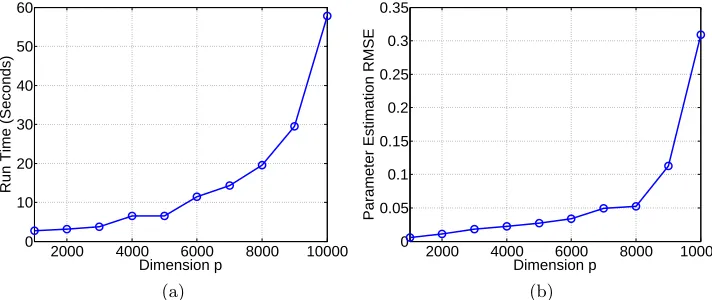
Figure 3: Scalability experiments on very large data sets on GPU using the fast approach. Accuracy results are normalized.
Figures 2b and 3 are obtained under the setting ofq= 10000,n= 5000,r= 1 and non-zero ratio of 10%. The results indicate that while SEED is fast on the GPU, it also achieves reasonable accuracy. Note that the results show that SEED is able to estimate a sparse and low-rank matrix with 108 elements in less than a minute, confirming its extreme scalability.
5.2. Real Data Analysis
Diffusion Network Inference, that is, the task of inferring influence networks from user activities, is one of the central tasks in social networks analysis (Gomez-Rodriguez et al., 2012) because it helps improve social marketing by finding the influential users in a network. It is a challenging problem because: (i) in many social networks the influence is expressed implicitly (Gomez-Rodriguez et al., 2012) and (ii) empirical studies show that common metrics such as number of friends or followers fail to accurately measure the social influence of the users (Cha et al., 2010).
A popular computational approach in estimating social influence among users is to count the number of users’ activities over a time span (in regularly or irregularly spaced intervals) and analyze the resulting time series data (Truccolo et al., 2005). Many different models have been developed, among which the vector auto-regressive model arises as a simple and robust solution (Trusov et al., 2009; Bahadori and Liu, 2013). That is, every user i is described by a time series xi(t) fort= 1, . . . , T and i= 1, . . . , q, such that
xi(t) = q
X
j=1
βTi,jxt,Laggedj +εi(t),
where βi,j is the vector of coefficients modeling the effects of time series xj, xt,Laggedj =
[xj(t−L), . . . , xj(t−1)]T is the history of xj up to time t with L the maximal time lag,
andεi(t) is the random noise at time t. Denoting by x(t) = [x1(t), . . . , xq(t)]T, we have the
following multi-response regression model:
1 2 3 4 5 0.45
0.5 0.55 0.6 0.65 0.7 0.75
Rank
Graph Recovery AUC
SEED RCGL LN-ADMM
M
Figure 4: The graph recovery accuracy of the algorithms as the rank of solution varies.
where the predictor vectorxt,Lagged= [(xt,Lagged1 )T, . . . ,(xt,Laggedq )T]T,BT = βTi,j
1≤i,j≤qis
the evolution matrix, andε(t) = [ε1(t), . . . , εq(t)]T. The influence network can be built from
the evolution matrix by establishing an edge from nodejto node iifkβi,jk1 is significantly larger than zero.
In this experiment, we gather a Twitter data set with tweets on the “Haiti earthquake” and apply vector auto-regressive model to identify the potential top influencers on this topic (that is, those Twitter accounts with the largest impact on the others). We divide the 17 days after the Haiti Earthquake on Jan. 12, 2010 into 1000 uniformly spaced intervals and generate a multivariate time series data set by counting the number of tweets on this topic for the top 1000 users who tweeted most about it. For accurate modeling, we remove the users that were highly correlated with each other, most of which were operated by the same users and tweeted exactly the same content. We also remove robot-like user-accounts which tweeted on very regular intervals, which in total led to a subset of 270 users. We analyze this data by a VAR model with the maximal time lag L= 5 based on the intuition about the maximum retweeting delay, which requires estimation of aq= 270 dimensional response vector usingp= 1350 predictors while we have onlyn= 995 observations.
Since we do not have access to the true influence network, we use the retweet network as a surrogate of the ground truth following the evaluation convention in the social networks community. The retweet network is constructed by adding an edge from user i to user j if user j has retweeted at least 4 of the tweets of user i. Clearly, the retweet network is not the actual underlying temporal dependency graph, mainly because there are possible implicit influence patterns as well. However, it is the best possible metric that we could obtain for graph estimation accuracy evaluation in our data set (Cha et al., 2010). The retweet network for the 270 selected users is sparse; it has only 0.11% of possible edges.
We apply SEED, ADMM, and RCGL algorithms to uncover the influence network in our twitter data set. Figure 4 shows the accuracy of the procedures in uncovering the true influence network in terms of AUC. For every value of the rank parameter, we tune the sparsity by 5-fold cross-validation. Given the fact that exact rank constraint cannot be enforced directly in the ADMM algorithm, we find the best value of the nuclear norm regularization parameter λL by 5-fold cross-validation. Then, we compute the low-rank
SEED ADMM RCGL
2.83 127.34 256.87
Table 2: Run time (in seconds) of the algorithms on the application data set.
The results in Figure 4 show that SEED significantly outperforms the baseline proce-dures. They also indicate that, in all of the algorithms, as we increase the rank of the solution matrix, the accuracy is improved initially and then quickly saturates. SEED achieves the highest accuracy when the rank is 4. Note that this result also confirms other studies that the social network connections may be strongly influenced by a few unobserved exogenous variables (Myers et al., 2012). The results in Table 2 demonstrate the significant speedup achieved by SEED compared to the baselines.
6. Discussion
In this paper, we propose to convert the problem of sparse reduced-rank regression into a sparse generalized eigenvalue problem, which allows us to efficiently employ the recently developed sparse eigenvalue decomposition techniques. After this transformation, the left singular vectors can be estimated in simple steps and the estimation of both sparse and dense right singular vectors is unified in a single framework. As a pure learning algorithm, SEED deviates from traditional regularization frameworks (that is, a loss function plus certain penalties), leading to computational efficiency and scalability. Furthermore, we prove that SEED achieves nice estimation and prediction accuracy similar to the minimax error bound in the univariate regression setting (Raskutti et al., 2011).
Some interesting problems for future research include extending the current formulation of the regression coefficient matrix in (2) to the case where the singular values can be repeated such that the left singular vectors (which correspond to latent factors) are not identifiable. Then we will need to estimate the eigenspaces spanned by important singular vectors and characterize the estimation accuracy by some new criterion, such as the one in Cai et al. (2013) and Ma (2013). Another research direction is to explore the theory of random design matrices and this can be addressed by using an extended version of perturbation theory (Lemma 6), where the perturbation inPis also included in the analysis.
Moreover, it is computationally straightforward to extend SEED to the generalized linear models by adapting the sequential quadratic programming framework. For this extension, we first approximate the loss function by the quadratic loss function and find the optimal unit rank matrix. Then we can add the unit rank matrix to the solution and re-approximate the loss function with another quadratic function around this new solution. By performing these three steps sequentially, we can efficiently estimate the low-rank coefficient matrix. Statistical properties of such estimator can be analyzed by extending the results in Lozano et al. (2011) for greedy sparse procedures to reduced-rank regression.
We would like to acknowledge support for this project from NSF CAREER Awards DMS-0955316 and IIS-1254206, NSFC-11601501, 11671374 and 71731010, Anhui Provincial Natu-ral Science Foundation-1708085QA02, Fundamental Research Funds for CentNatu-ral Universities-WK2040160028, Okawa Foundation Research Award, a grant from the Simons Foundation, and Adobe Data Science Research Award. The authors would like to thank Emre Demirkaya and Sanjay Purushotham for helpful discussions. The authors also sincerely thank the Action Editor and referees for their valuable comments that helped improve the article substantially.
Appendix A. Proofs of Theorems 1 and 2
We need the following two lemmas in the proofs of Theorems 1 and 2.
Lemma 5 Suppose ε ∼ N(0q,Σ) and γ2 = maxjΣjj. We have stacked n realization of
these random vectors in the rows of n×q matrix E. Denote by P2 = max
j[1nXTX]jj given
a deterministic n×p matrix X. Then for anyδ ∈(0,1), with probability at least 1−δ, 1
nkE TXk
2,s ≤
r
2qs(γP)2
n log
2pq δ .
Lemma 6 (Perturbation Theory for Sparse Symmetric Generalized Eigenvalue Problems) Suppose Q,P ∈ S+p are two p×p semi-definite matrices. For the following generalized
eigenvalue problem and its perturbed variant with sparse eigenvectors
Qu=λPu, (10)
(Q+δQ)bu=bλPub, (11)
where u,bu ⊥ Ker(P) with kuk0 ≤ s
∗, k
b
uk0 ≤ s and s∗ < s, under Condition 1, we have uniformly over k= 1,· · · , p−dim{Ker(P)},
|λbk−λk| ≤φs−1kδQk2,s. (12)
Here λk and λbk are the kth largest eigenvalues of equations (10) and (11), respectively,
kδQk2,s denotes the s-sparse largest singular value of δQ, andφs is defined in Condition 1.
Furthermore, denote by uk andubk the unit length sparse eigenvectors correspond to λk
and bλk, respectively, with ukb taking the correct directions. When there exists some positive
eigengapdλ which is the minimum difference between non-zero eigenvalues of equation (10)
and the perturbation ofQsatisfieskδQk2,s =o(dλ), then uniformly overksuch thatλk 6= 0,
kubk−ukk2≤ √
2φ−s2d−λ1kδQk2,s+o(d−λ1kδQk2,s). (13) A.1. Proof of Theorem 1
the eigenvalue perturbation theory (Lemma 6), we derive the error bound forubk. Using the
bound forukb , in the third step, the error bound forbvk is calculated.
Step 1: Bounding the perturbation of matrix Q. For notational simplicity, define the noise free response variables as Y∗ = XC∗, Q = qn12X
TY∗Y∗TX and its noisy version
b
Q = qn12X
TYYTX. Denote by k
b
Q−Qk2,s the s-sparse largest singular value of Qb −Q.
Since Y=Y∗+E, we can derive the following bound,
kQb −Qk2,s =
1 qn2
X
TYYTX−XTY∗Y∗T X
2,s ≤
2 n2q
XTY∗ETX 2,s+
1 n2qkE
TXk2 2,s,
where the last inequality is due to the expansion of XTYYTX and an application of the triangular inequality.
By Condition 1 and Proposition 1, we have kXk2,s ≤
√
nφ−s1/2 and
kXTY∗k2≤ kXk2,s· kY∗k2 =kXk2,s·√nqσ1≤n √
qσ1φ−s1/2, (14)
where the first inequality holds since the unit length vector v satisfying kXTY∗vk2 = kXTY∗k2 must be one of the v∗k in (2) due to the strict separation of the singular values by Condition 2, so that XTY∗v∗k =XTXC∗v∗k with C∗v∗k yielding an s-sparse vector for
XTX. Therefore, we get
2 n2q
XTY∗ETX
2,s ≤
2 n2q
XTY∗
2·
ETX
2,s≤
2σ1φ−s1/2 n√q
ETX
2,s.
Leta∗ =σ1φ
−1/2
s . It follows that
kQb −Qk2,s ≤
2a∗ n√qkE
TXk
2,s+
1 n2qkE
TXk2
2,s. (15)
Step 2: Error bounds for ukb and Xbuk. Using Lemma 5, for any δ ∈(0,1) with
proba-bility at least 1−δ, we have
1 n√qkE
TXk
2,s≤γP
r
2s n log
2pq δ .
Since snlogpqδ →0 , substituting the above bound in equation (15) yields
kQb −Qk2,s ≤γP a∗ r
8s n log
2pq δ +o
r s nlog pq δ . (16)
Therefore, under Conditions 1 and 2, applying Lemma 6 with Qb = 1
qn2X
TYYTX,
Q= qn12XTY
∗Y∗TX, and P= 1
nX
TX gives the following bound for
b
uk,
kubk−u∗kk2≤
4γP a∗ dσφ2s
r
s nlog
pq δ +o
r s nlog pq δ
=Cu
r
s nlog
pq δ +o
whereCu= 4γP a ∗
dσφ2s =
4γP σ1 dσφ5s/2
is a constant. Sincekubk−ukk0 ≤2s, further applying Condition 1 yields
1
√
nkX(buk−u
∗
k)k2≤φ
−1/2
s Cu
r
s nlog
pq δ +o
r s nlog pq δ .
Step 3: Error bound for vbk. With the estimated left singular vector ubk, we can further
estimate the corresponding right singular vector as
b
vk=
1
b
u>kXTXukb
YTXubk,
and compare it to v∗k, which by Proposition 1 can be expressed as
vk∗ = 1
u∗>k XTXu∗kY ∗T
Xu∗k.
For simplicity of notation, we drop the index kof vk and uk and write
kvb−v∗k2 =
1
u∗>XTXu∗−e1
Y∗TXu∗−e2
− 1
u∗>XTXu∗Y ∗T Xu∗ 2 ,
wheree1 ,u∗>XTXu∗−ub
>XTX
b
uande2 ,Y∗TXu∗−YTXub. Using the Taylor expansion
of 1−x1 atx= 0, we can write
kvb−v∗k2≤
Y∗TXu∗ u∗>XTXu∗
e1
u∗>XTXu∗
2 + e2
u∗>XTXu∗
2
+Te
= (u∗>XTXu∗/n)−1(kv∗k2|e1|/n+ke2k2/n) +Te
≤φ−s1(kv∗k2|e1|/n+ke2k2/n) +Te, (17)
whereTe=
k
v∗k2|e1|/n
u∗>Pu∗ +
ke2k2/n
u∗>Pu∗
P∞
`=1
|e1|/n
u∗>Pu∗
`
denotes the higher order terms in the Taylor expansion and the last step is by Condition 1.
Bounding |e1|: Let ub = u
∗ +δ
u. Since ku∗k0 ≤ s∗, kubk0 ≤ s and s
∗ < s, we have
kδuk0 ≤2s. Asu∗ is a unit length vector, it yields from Condition 1 that |e1|/n=
1 n(u
∗+δ
u)>XTX(u∗+δu)−
1 nu
∗>XTXu∗
=|2u∗>Pδu+δTuPδu| ≤φs−1(2kδuk2+kδuk22). (18) Bounding ke2k2: Similarly, let YTX=Y∗TX+ETX. We obtain
ke2k2/n=k(Y∗TX+ETX)(u∗+δu)−Y∗TXu∗k2/n ≤ kY∗TXδuk2/n+kETXu∗k2/n+kETXδuk2/n
where in the last step we used kY∗TXδuk2/n≤a∗ √
qkδuk2 similarly as in (14). Since √1
qkv ∗
kk2 ≤ V, substituting inequalities (18) and (19) in inequality (17) with reorganization yields
kvbk−v∗kk2 ≤
V√qkδuk2
φ2
s
2 +kδuk2
+ 1
nφs
kETXk2,s(1 +kδuk2) +φ−s1a∗√qkδuk2+Te.
When slog(pq/δ) = o(n), we can see that both the events E1 =
n
kδuk2 =O
q s nlog pq δ o
and E2 =
n
Te=O
q qs n log pq δ o
occur, if the eventE0=
n
1
n√qkE TXk
2,s =O
q s nlog pq δ o
holds for someδ∈(0,1), where in the second event we have used the results in inequalities (18) and (19) together with an application of geometric series sum. Note that the first term
of Te is O
q qs n log pq δ
and the common ratio isOqns logpqδ .
Therefore, by applying the result in Lemma 5 for bounding kETXk2,s/nand the result for the estimation error bound ofkubk−u∗kk2 inStep 2, we can conclude with probability at least 1−δ that
kvbk−v∗kk2 ≤
(2V φ−s1+a∗)Cu+γP φs
r
2qs n log
pq δ +o
r qs n log pq δ
+Te
≤ 2{(2V φ
−1
s +a∗)Cu+γP} φs
r
2qs n log
pq δ +o
r qs n log pq δ
=Cv
r
qs n log
pq δ +o
r qs n log pq δ ,
whereCv = 2
√
2φ−s1n(2V φs−1/2+σ1)φ
−1/2
s Cu+γP
o
.
Step 4: Error bounds for √1
qkCbk−C ∗
kkF and √1qnkX(Cbk−C∗k)kF. With the estimation
error bounds of buk and vbk, we write
1 qnkX(C
∗
k−Cbk)k2F =
1
qtrace{(C ∗
k−Cbk)TP(C∗k−Cbk)}= ˜e1+ ˜e2+ ˜e3, (20)
where the last equality follows from the decomposition
C∗k−Cbk=u∗kv∗Tk −ubkbvTk = (u∗k−ubk)v∗Tk +ubk(v∗k−bvk)T (21)
such that
˜ e1 =
1
qtrace{v ∗ k(u
∗ k−ukb )
TP(u∗
k−ukb )v
∗T k },
˜ e2 =
2
qtrace{(v ∗
k−vkb )ub
T jP(u
∗
k−ukb )v
∗T k },
˜ e3 =
1
qtrace{(v ∗
k−vkb )ub
T kPbuk(v
∗ k−bvk)
We will bound them separately. Since the estimation error bounds of ubk and bvk, k=
1,· · · , r∗, hold with probability at least 1−δ. It yields that
˜ e1 =
1
qtrace{(u ∗ k−buk)
TP(u∗
k−buk)v
∗T k v
∗
k}=V2·(u ∗ k−ukb )
TP(u∗ k−ukb )
≤V2φ−s1ku∗k−ubkk22 ≤V2φ−s1Cu2
s nlog pq δ +o s nlog pq δ ,
where the first inequality follows from Condition 1 and the factku∗k−ukb k0 ≤2s. Similarly, we have
˜
e2 ≤2V φ−s1CuCv
s
nlog pq
δ
+os nlog pq δ , ˜
e3 ≤φ−s1Cv2
s
nlog pq
δ
+os nlog
pq δ
.
In view of (20), the above bounds together give
1
qnkX(Cbk−C ∗
k)k2F ≤φ −1
s (V Cu+Cv)2
s nlog pq δ +o s nlog pq δ .
Thus we have
1
√
qnkX(Cbk−C ∗ k)kF ≤
(V Cu+Cv)
φ1s/2
r s nlog pq δ +o r s nlog pq δ .
By a similar but simpler argument, it follows from the decomposition (21) that
1
√
qkC ∗
k−CbkkF ≤
1
√
qk(u ∗
k−buk)v
∗T k kF +
1
√
qkubk(v
∗ k−vbk)
Tk F
= √1
qku ∗
k−ubkk2· kv
∗ kk2+
1
√
qkbukk2· kv
∗
k−bvkk2
≤(V Cu+Cv)
r s nlog pq δ +o r s nlog pq δ .
It concludes the proof.
A.2. Proof of Theorem 2
The main idea for proving the rank consistency result is noting thatbσk2= (ub>kQbubk)/(ub>kPubk)
which relates to the termination criteria is in fact thekth largest eigenvalue of the problem
b
Qu= λPu. Thus, we will show that the amount of decrease in the objective function in thekth step equals to the thekth largest eigenvalue of the problemQub =λPu. Given the
perturbation bounds in Lemma 6, we can bound its difference from the true eigenvalue and show that after r∗ greedy steps, the eigenvalues become almost zero.
To prove the result in Theorem 2, we need to bound logLk−1 −logLk, where Lk =
1
nqkY−XCkk2F is the objective function with Ck = Pkj=1Cbj the estimated coefficient
matrix up to thekth step. By using the fact that 1−1
x ≤log(x)≤x−1 forx >0, we can
write
Lk−1− Lk
Lk−1
≤log
L
k−1 Lk
≤ Lk−1− Lk Lk
Next, we show that the amount of the decrease in the objective function in the kth step is equal to the the kth largest eigenvalue of the problem Qub = λPu, which satisfies the
following equality
Lk−1− Lk=
1
nqkY−XCk−1k
2
F −
1
nqkY−XCkk
2
F
= 1
nqkY−XCk−1k
2
F −
1
nqkY−XCk−1−Xubkvb
> kk2F
= 1 nq
2DY−XCk−1,Xubkbv
> k
E
− kXbukbv
> kk2F
.
Now, using the P-orthogonality ofbuk’s, we have
Lk−1− Lk=
1 nq
2
D
Y,Xubkvb
> k
E
− kXubkvb
> kk2F
= 1 nq 2
b
u>kXTYYTXukb
b
u>kXTXukb
−ub
> kX
TYYTX
b
uk
b
u>kXTXbuk !
= ub
> kQbubk b
u>kPbuk
=σb
2
k,
where the second step is due to the substitution of the solution forvkb in (6) and a few steps
of algebraic rearrangement.
Underfitted regimek≤r∗. Under Condition 1, using the perturbation bound in Lemma 6 for the eigenvaluesσ2k’s withk≤r∗, we can write
b
σk2≥σk2−φs−1k∆Qk2,s.
Further applying inequality (16), we know that there exists some positive constantC such that
φ−s1k∆Qk2,s ≤2a∗φ−s1γP
r
2s n log
pq δ +o
r s nlog pq δ ≤C r s nlog pq δ .
Therefore, it follows that with probability at least 1−δ,
b
σ2k≥σ2k−C
r
s nlog
pq
δ . (22)
Then we can derive the following lower bound
s
Lk−1− Lk
Lk−1 ≥
r
σk2−C
q s nlog pq δ 1 √ nq Pr∗
j=kkXC ∗
jkF +Pk−j=11kX(C
∗
j −Cbj)kF +kEkF
, (23)
where C∗j =u∗jv∗Tj , Cbj =ubjvbj, in the nominator we have used the result obtained in (22)