* Corresponding author.
E-mail: [email protected] (M. M. Saffar) © 2014 Growing Science Ltd. All rights reserved. doi: 10.5267/j.ijiec.2014.10.001
International Journal of Industrial Engineering Computations 6 (2015) 15–32
Contents lists available at GrowingScience
International Journal of Industrial Engineering Computations
homepage: www.GrowingScience.com/ijiecA new multi objective optimization model for designing a green supply chain
network under uncertainty
Mohammad Mahdi Saffar*, Hamed Shakouri G. and Jafar Razmi
Department of Industrial Engineering, College of Engineering, University of Tehran, Tehran, Iran
C H R O N I C L E A B S T R A C T
Article history: Received June 6 2014 Received in Revised Format September 9 2014
Accepted October 2 2014 Available online October 3 2014
Recently, researchers have focused on how to minimize the negative effects of industrial activities on environment. Consequently, they work on mathematical models, which minimize the environmental issues as well as optimizing the costs. In the field of supply chain network design, most managers consider economic and environmental issues, simultaneously. This paper introduces a bi-objective supply chain network design, which uses fuzzy programming to obtain the capability of resisting uncertain conditions. The design considers production, recovery, and distribution centers. The advantage of using this model includes the optimal facilities, locating them and assigning the optimal facilities to them. It also chooses the type and the number of technologies, which must be bought. The fuzzy programming converts the multi objective model to an auxiliary crisp model by Jimenez approach and solves it with -constraint. For solving large size problems, the Multi Objective Differential Evolutionary algorithm (MODE) is applied.
© 2015 Growing Science Ltd. All rights reserved Keywords:
Reverse supply chain CO2 emission
Uncertainty Jimenez method Multi objective differential evolutionary algorithm
1. Introduction
Supply chain management includes managing production and supply processes, from raw material to final customers as well as considering the whole supply chain network from the beginning to the end of the useful life of the product. Some researchers and organizations not only consider the above definition they also think about raw materials and their role in supply chain management, supply of resources processes, construction, and transportation in supply chain networks. Supply chain networks contain forward flows and backward ones, such as discounts, persuasive payments, information flows, and collecting the impaired product from customer zones. Consequently, decisions are made in three levels of strategic decisions, tactical decisions, and operational decisions.
1.1. Strategic decisions
1.2 Tactical decisions
Medium planning decisions particularly determining the inventory levels, discount planning, choosing suppliers in each market are made in this level. The time intervals of the decisions in this level are varied from three months to one year and predicting process are more specified than strategic levels and moreover, organizations prescribe a set of policies.
1.3 Operational level
The lifespan of these kinds of decisions are from one day to one week and they are made on the foundation of customers’ demands. Short time planning focuses on how to assign products to customers, deciding the date of satisfying orders, and scheduling the time for vehicles. By making new rules related to wastage and produced commodity, especially in Europe, producers have developed their processes and become responsible for collecting, distributing, and updating their second hand commodities. Apart from that, in order to motivate and improve a logistic system, it is required to consider reverse distribution, and reverse logistics to satisfy customer. This happens in a way that customers are assured that the logistic system is secure enough to meet their demands and in case of any fault and defect in distributed products, by using reverse logistics in a mean time, the perfect ones superseded the defective ones. Among the most important decisions in supply chain, there are the strategic level decisions and what really matters in supply chain strategic design is locating facilities and then relating the located facilities based on the design. Melkote and Daskin (2001) represent a single-period locating-network designing model considering capacity constraints. In this model, each vertex is a demand center and only one facility, which has a limited capacity, is permitted to be assigned to each vertex. The objective function minimizes the cost of transportation, locating the facilities, and allocations. Thanh et al. (2008) introduce a dynamic model under uncertainty in which various parameters such as demands, selling prices, and cost of funding facilities in different periods are contemplated. Drenzner and Wesolowsky (2003) in their paper introduce a period single-layer location model. Furthermore, Ambrosino and Acutella (2005) study a dynamic multi-single-layer model including the layer of factory, the layer of central distribution centers, the layer of regional distribution centers, and the layer of demands. In the paper of Ozdemir et al. (2006), a two-layer model considering capacity constraints is depicted whereby the total costs are minimized as well as choosing the optimal allocation. The model of Pirkal and Jyraman (1998) is multi product supply chain design. One of the significant specifications in supply networks is the flow of goods with defects and faults. In recent years, some papers mention flows, consider spoil of inventory items, receiving defective goods from customers, and therefore create a backward flow in supply chain network. Some other papers take both, forward and backward, flows into account and introduce an integrated flow. For example, as initial works in reverse supply chain network design problem, Fleischmann et al. (1997) introduce a comprehensive survey on the application of mathematical modeling in reverse supply chain management. Barros et al. (1998) present a MILP model for a sand recycling network solved by a heuristic algorithm. Jayaraman et al. (1999) present a MILP model for reverse supply chain network design based on customer demands for recovered products. The goal of the presented model is to minimize the traditional costs. Jayaraman et al. (2003) develop their previous work to model the single product two-level hierarchical location problem considering the reverse logistics operations of hazardous products. They also extend a heuristic to solve large-sized problem. Pati et al. (2008) introduce a mixed-integer goal programming model for paper recycling supply chain network design. The aims of objective functions are: (1) minimizing the positive deviation from the specified budget (2) minimizing the negative deviation from the minimum planned waste collection and (3) minimizing the positive deviation from the maximum limit of wastepaper. Krikke et al. (1999) propose a MILP model for a two-stage reverse logistics network.
multi-product dynamic model. In addition, Lu and Bostel (2007) represent a three-layer designing model, which locate facilities in the reverse logistics networks optimally. Pishvaee et al. (2011) introduce a linear model minimizing transportation costs. Moreover, Pishvaee et al. (2012) provide a model considering both forward and backward flows, simultaneously. The design of forward and reverse logistics networks has a strong impact on the performance of each other. Thus, to avoid the sub-optimality caused by the separated design, the design of the forward and reverse supply chain networks should be integrated (Pishvaee et al., 2010; Fleischmann et al., 2001). Salema et al. (2007) develop the Fleischmann et al. (2001) model by using stochastic mixed-integer programming approach under uncertainty. Lu and Bostel (2007) propose a mixed-integer programming model including both forward and reverse networks and their interactions simultaneously and to solve the presented model, they use Lagrangian-based heuristic. Klibi et al. (2010) conduct a survey on supply chain network design problems to demonstrate future research directions. Pishvaee et al. (2010) propose a bi-objective mixed-integer linear programming model minimizing the total costs in a closed-loop logistics and maximizing the network responsiveness. A memetic algorithm is extended to solve the presented bi-objective MILP model. Thus, by using integrated design of forward and reverse supply chain networks the profits results are taken and the whole life cycle of good and product are supported. General models (e.g. Wang & Hsu, 2010b) and case-based (e.g. Ko & Evans (2007)) are proposed by researchers. The imprecise nature of returned products causes a high degree of uncertainty in closed-loop and reverse supply chain network design problems.
Ilgin and Gupta (2010) present a comprehensive review on company's conscious about environment and product recycle and recovery and they survey some affiliate papers that work on environmental supply chain network design. Since the end-of-life (EOL) goods and products have important impact on environment, this has created a need to extend and develop models for reverse supply chain (logistics) network design. Additionally, as seen in relevant literature, a thin part of works incorporates the environmental issues into supply chain network design decisions. Hugo and Pistikopoulos (2005) present a bi-objective mathematical programming model to consist environmental impact in forward supply chain network problem. The proposed model maximizing the total profit and moreover, minimizes the environmental impact by applying LCA principles. For electronic equipment recycling network a model is presented by Quariguasi Frota Neto et al. (2009) to minimize traditional cost objective in addition to cumulative energy demand and wastes. Quariguasi Frota Neto et al. (2008) proposed a bi-objective linear programming model for forward supply chain network design considering environmental impacts in European pulp and paper industry. However, the developed model is able to optimize the quantity of flow between supply chain layers and ignores the other decisions such as determining the location, number of facilities and capacity of them. All of the mentioned papers in the area of environmental supply chain network design avoid the integrated design of forward and reverse networks and incorporating the environmental issues into decision making model. In addition, all of the above mentioned papers are incapable to model the uncertainty of parameters in supply chain network design problem. To cope with this uncertainty issues, most of the relevant papers applied stochastic programming approaches (e.g. Pishvaee et al., 2009; El-Sayed et al., 2010). Because of the lack of historical data in real cases that is rarely available and the high computational complexity, the use of stochastic programming models seems to be impossible for real cases. Therefore, in recent years, a few number of papers use more flexible approaches such as fuzzy programming (e.g. Wang & Hsu, 2010a). El-Sayed et al. (2010) present an integrated designing network under probabilistic approaches, which determined distribution centers, suppliers, re-assembly centers, and re-distribution centers. Furthermore, Qin and Jin (2009) consider the rate of reverse products, their quality levels for being useable or recycling under uncertainty.
improve the results of first stage with four movements. Syam (2002) apply simulated annealing operation to solve the model considering logistic costs in supply chain. Table 1 shows the characteristic of some papers regarding to literature review are studied to find the research gap.
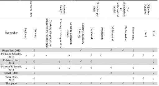
Table 1
The summary of literature review and research gap Network Flow
Network
Design
Green supply
chain The
chara
cte
ris
tic
of
math
ema
tic
al
model Object
ive
Function
Researcher
Backward Forwa
rd
Choosing the pr
oduction
and recovery
technologies
Loca
ting r
ecov
ery
cen
ters
Loca
ting Co
lle
ct
ion
cent
ers
Locating Inv
entory
loca
ting
Backward. Production Multi-period Multi-product Uncerta
inty
F
uel Cost
Baghalian, 2013 √ √ √ √ √ √
Pishvaee &Razmi,
2013 √ √ √ √ √ √ √ √ √
Pishvaee et al.,
2011 √ √ √ √ √ √ √
Pishvae & Torabi,
2011 √ √ √ √ √ √ √ √ √
Sawik, 2011 √ √ √ √
Shaw et al.,
2013 √ √ √ √ √
This paper √ √ √ √ √ √ √ √ √ √ √ √ √
As in Table 1 there is no paper, which considers environmental issues in the form of recovery, production, and reverse network- and economic cost simultaneously and design the supply chain network with real hypotheses and quite a few uncertain parameters.
2. Problem Definition
Based on Fig. 1, the supply chain network studied in this paper, distributes goods among customers from distribution centers.
Fig. 1. The structure of the proposed study
Production centers
Customer centers
Collection and examination centers Distribution
centers
Recovery center
Then, product, after being defective, are returned to supply chain and after examination, the recoverable products are sent to recovery centers and the remains are sent to material customers. In recovery centers, after maintaining the products, they are returned to distribution centers to be sent to customer zones. The model considers the cost of locating facilities, transportation costs, the cost of production and maintenance, rate of CO2 emission related to production, maintenance, and operation,
the time machines are available, rate of returned products, rate of recoverability, by reason of being uncertain in real problems are considered in form of fuzzy parameters. Fuzzy indexes are shown with the sign “~”on top of them.
Model assumptions
Each facility has a limited capacity.
The locations of customer zones and the material customers are fixed and predicted. All demands should be met.
The potential location of distribution centers, collection centers, and recovery centers are discrete.
The model is multi-product multi-period.
The amount of CO2 emission of production and recovery are uncertain.
In each layer, it is possible to use from several or all centers of that layer.
The probability that a defective product is sent to a customer is more than zero and this product is sent to collection center.
The output of the model
The model looks for optimal locations of collection and examination centers, and recovery centers.
The optimal flows of goods among all facilities are related altogether.
The model determines the number of machines from each technology for production and recovery centers.
The model determines the types of products and how many of them produced or recovered by the chosen machines.
The model determines how much of salvage materials are sold to which customers. The indexes, parameters, and decision variables are as follows:
Indices and sets
j Index of different parts, j0,1, , J
r Index of candidate locations for the distribution centers,r0,1, , R
v Index of fixed locations for the material costumer zones, v1, 2,,V
k Index of fixed locations for the costumer zones, k1, 2,,K
q Index of candidate locations for the collection centers, q1, 2,,Q
m Index of candidate locations for the recovery centers, m1, 2,,M
z Index of capacity levels available for distribution centers, z1, 2,,Z
l Index of different technologies available for production centers, l1, 2,,L
o Index of different technologies available for recovery centers, o1, 2,,O
Parameters
z r
H Fixed cost of opening distribution center r with capacity level z
q
h Fixed cost of opening collection center q
m
r Fixed cost of opening recovery center m
l
Cs Purchasing cost per machine with l technology in the plant
o m
Cs Purchasing cost per machine with o technology at recovery center m
l j
h Producing cost per unit j produced in the plant with technology l
o jm
Remanufacturing cost per unit j at recovery center m with technology o
jr
c Transportation cost for shipping one product unit j from plant to distribution center r
jrk
a Transportation cost for shipping one product unit j from distribution center r to costumer
zone k
jkq
b Transportation cost for shipping one product unit j of returned products from customer zone k to collection center q
jqm
v Transportation cost for shipping one product unit j of recoverable products from
collection center q to recovery center m
jmr
s Transportation cost for shipping one product unit j of recovered products from recovery
center m to distribution center r
jqv
V Transportation cost for shipping one product unit j from collection center q to raw material customer v
l
Ti Available time for one machine with l technology in plant
l j
Pt Time needed for producing one product unit j with l technology in plant
o
TM Available time for one machine with o technology in recovery center
o j
PTM Time needed for recovering one product unit j with o technology in recovery center
ji
C
Capacity of supplier i for producing part jz r
V oR Available volume for keeping parts of distribution center r with capacity level z
l j
L CO2 equivalent emission per unit product j produced by the plant with technology l
o j
CO2 equivalent emission per unit product j recovered with technology o
jkt
Rate of return percentage product type j from customer zone k in period t
jkt
r Amount of returned product unit j to customer center k in period t
j
Rate of recoverable percentage product type j
jv
Co Price per unit of product j in raw material costumer v
jkt
d
Demand of costumer zone k for product j in period t jV o Volume of one unit of product j Decision variables
jrt
y Quantity of parts j shipped from plant to distribution center r in period t
jrkt
Quantity of part j shipped from distribution center r to customer zone k by in period t
jkqt
Quantity of returned products j shipped from customer zone k to collection center q
jqmt
M Quantity of collected products j shipped from collection center q to recovery center m
in period t
jmrt
Quantity of recovered products j shipped from recovery center m to distribution center m by transportation mode p at period t
jqvt
U Quantity of salvaged products j shipped from collection centers q to material costumer
zone v in period t
l jt
z Quantity of products j manufactured in the plant with technology l in period t
l
NM Number of purchased machines with l technology in the plant mo
jmt Quantity of collected products j in recovery center m that recovered with o technology
in period t
o m
NoM Number of purchased machines with o technology in recovery center m
z r
= 1 if a distribution center with capacity level z is opened at location r; 0, otherwise
q
z =1 if a collection center is opened at location q; 0, otherwise
m
=1 if a recovery center is opened at location m; 0, otherwise
3. The proposed fuzzy model
A
Facility location fixed cost
. . .
z z
r r q q m m
r z q m
H
h z
r
B
The cost of buying production and maintaining machine .
.
l l o o
m m
l l
NM Cs
Cs NoM
C
Production and recovery costs
. .
l l o o
jt j jmt jm
l j t m o j t
z
h
m
D
Transportation costs
. .
. .
. .
jrt jr jrkt jrk
r j t r k j t
jkqt jkq jqmt jqm
k q j t q m j t
jmrt jmr jqvt jqv
m r j t q v j t
y c
a
b
M
v
s
U
V
E
Income of selling salvaged products
.
jqvt jv
q v j t
U
Co
(1) First objective function: total
costs
(2) Second objective function: CO2
emission costs
subject to
Decision Variable Constraints
(3)
, ,
j t k
(4) , l t (5) , j t (6) , ,
r j t
(7)
, ,
k j t
(8)
, ,
q j t
(9)
, ,
q j t
(10)
, ,
m j t
(11)
, ,
j m t
(12) , r t (13) , ,
m o t
(14) r (15) q
(16) m
(17)
, ,
0,1
, , , ,
zr
z
q mr z q m
min ljt. lj ojmt. oj
l j t m o j t
z L
m
r d jrkt jkt
. .l l l l
jt j j
Z Pt NM Ti
= y l jt jrt l r z
jrt jmrt jrkt
m k
y
. ( 1)
jkqt jkt jkt q
jk t
r
d
jkqt jqmt jqvt
k m v
M U
.
j jkqt jqmt
k m M
jqmt jmrt q rM
o
jmt jqmt
o q
m M
. z. z
jrkt j r r
j k z
V o V oR
. .o o o o
jmt j m
j
m PTM TM NoM
1 z r z
. jkqt q k j tM z
.
o
jqmt m m
q j t o
M NoM M
The first objective function minimizes total costs and the second objective function minimizes the CO2
emissions. The constraint (3) ensures that customer demands for each type of products must be met, considering production limit and available time limits. Constraint (4) assures that the productions of factory is less than its capacity, constraint (5) strikes a balance between the input and the output of the distribution centers. Constraint (6) indicates the equivalent of input and output of customer centers, considering rate of returned goods of previous periods. Constraint (8) ensures that the input and output of collection centers are equal. Constraint (9) divides defective goods into recoverable goods and unrecoverable ones, based on the rate of recoverable defective good. Constraints (10) depict the balance between input and output of recovery centers. Constraint (11) assures that all products must be repaired by one type of technologies. Constraint (12) ensures that the volume of products in distribution centers are less than the distribution centers capacity. Constraint (13) ensures that unless a technology is not bought, no product is repaired with that technology. Constraint (14) assures that if in a candidate location a distribution center is constructed, it uses one type of capacity level. Constraint (15) ensures if a collection center is not constructed no product will be sent to it. Constraint (16) assures if a recovery center is not constructed, no product will be sent to it and o technology will be bought for it.
4. Solution procedure
The mathematical model for solving the mixed integer linear programming problem is a multi- objective fuzzy programming model. This two-stage approach is introduced by Jimenez et al. (1996). In the first stage, the model converts to a deterministic slack multi objective model and then, in the second stage, the -constraint process gives the final output to the decision makers.
The first step: a definite slack multi objective model for the fuzzy model:
This method is based on common ranking, which was introduced by Jimenez et al. (1996). What makes this model applicable is its applicability on stochastic parameters with different fuzzy functions whether they are symmetric or not. Such concepts as expected interval and expected value are the milestones of this method. First, these concepts were represented by Yager (1981). In order to introduce of these concepts triangle fuzzy number ( ,p m, )o
c c c c is considered and its membership
function is explained as follow:
(20)
Expected interval (EI) and expected value (EV) for the triangle fuzzy number care as follow:
(21)
(22)
(18)
(19)
, , m , , , , , .
l l o o
jt jmt m
z NM NoM Z l j t o m
, , , , , , , , , , , ,
jrt jrkt jkqt jqmt jmrt jqvt
y M U Z j r t k q m v
( )
1 ( )
( ) 0
p
p m
m p
m o
m o
o m
p o
x c
fc x if c x c
c c
if x c
x
c c x
gc x if c x c
c c
if x c or x c
1 1
1 1
2
0 0
1 ( ) ( )
( ) 1
2
1
,
,
(
), (
)
2
c p m m o
c c
c
x dx x dx
c c
EI
E E
f
g
c
c
c
1 2
( )
2
2
4
c c p m o
c
E
E
c
c
c
Apart from that, for each pair fuzzy number such as
a
andb
, the degree ofa
, which is greater thanb
is as follows,
2 1 2 1
1 2 2 1
2 1 1 2
1 2
0 0
( , ) 0
( )
1 0
a b a b
a b a b
M a b a b
a b
if E E E E
a b if E E E E
E E E E
if E E
(23)
where
M ( , )a b indicates the degree ofa
, which is greater thanb
. When it is said
M ( , )a b
itmeans
a
is at least greater thanb
with
degree shown asa b. Apart from that, for each pair of fuzzy numbera
andb
, it is saida
is equal tob
with
degree if these two formulas exist, simultaneously:(24)
Or
(25)
Now, we consider a fuzzy mathematical programming model in which all parameters are defined as triangular fuzzy numbers.
min ( )
subject to
, 1,...,
, 1 1,...,
0 t
i i
i i
z c x
a x b i l
a x b i m
x
(26)
According to Jimenez et al. (1996), a vector n
x R with degree
is feasible if
1,....
mini m
M (a x bi , )i
and according to Eq. (24) and Eq. (25) the a xi bi and a xi bi areequivalent to:
2 1
2 1 2 1
, 1,...,
i i
i i i i
a x b
a x a x b b
E E
i l
E E E E
(27)
2 1
2 1 2 1
1 , 1,...,
2 2
i i
i i i i
a x b
a x a x b b
E E
i l m
E E E E
(28)
which can be replaced by:
2 1 2 1
(1
)Eai
Eai x
Ebi (1
)Ebi, i 1,...,l
(29)
2 1 2 1
(1 ) (1 ) , 1,...,
2 2 2 2
i i i i
a a b b
E E x E E i l m
(30)
2 (1 ) 1 (1 ) 2 1 , 1,...,
2 2 2 2
i i i i
a a b b
E E x E E i l m
(31)
2
,
2a
b
a
b
( , ) 1
2 M a b 2
By using Jimenez et al. (1996) ranking method, it is proved that a feasible solution such as x 0 is an
optimal solution of the model (26) with
-acceptance if and only if X such that a xi bi for i 1,...,l and a xi bi for i l 1,...,m and x 0 holds the following equation:0 1 2
( ) ( )
t t
c x c x (32)
So under this circumstances, 0
x with at least ½ degree has a better solution than other feasible
solutions. The above equation can be rewritten as follows:
0 0
2 1 2 1
2 2
t t t t
c x c x c x c x
E E E E
(33)
Hence, by applying the concepts of excepted interval and excepted value for fuzzy numbers, the deterministic slack model can be rewritten as follows:
min
EV c x
( )
2 1 2 1
2 1 2 1
2 1 2 1
subject to
(1 ) (1 ) , 1,...,
(1 ) (1 ) , 1,...,
2 2 2 2
(1 ) (1 ) , 1,...,
2 2 2 2
0
i i i i
i i i i
i i i i
a a b b
a a b b
a a b b
E E x E E i l
E E x E E i l m
E E x E E i l m
x
(34)
Auxiliary Crisp Model
Based on the mentioned descriptions the model in this paper is converted to an auxiliary crisp model:
T
he num
ber
of
equation in f
uzzy
m
odel
T
he num
ber
of
equation in
auxiliary crisp
m
odel
A
A
0
2
2 2
. . .
4 4 4
p m p m o p m o
z z z
q q q
z
r r r m m m
r q m
r z q m
h h h
H H H r r r
Z
C C
2 2
. .
4 m 4
l j t m o j t
p m o
p m o
o o o
l l l
j j j jm jm jm
l o
jt jm t
h h h
z
. . 1 . ,2 2
. . 1 .
2 2
l
l l p l
m o m
j j j j
l jt r
p m m o
l l l l
l i
NM Ti T Ti Ti l t
Pt Pt Pt Pt
Z
DD
2 2
. .
4 4
r j t q m j t
p
p m o m o
jr jr jr jrk jrk jrk
jrt jrkt
a a a
c c c
y
+ 2 2 . . 4 4k q j t q v j t
p m o p m o
jkq jkq jkq jqm jqm jqm
jqmt jkqt
b b b v v v
M
+ . 2 . 2
4 4
r j t q m j t
p m o p m o
jmr jmr jmr jqv jqv jqv
jmrt jqvt
s s s V V V
U
EE
2 .
4
q v j t
p m o
jv jv jv
jq v t
C o
C o
C o
U
(1)
(35)
min A B CDE
(2)
(36)
(3)
(37)
(4)
(38)
(7)
(39)
(9)
(40)
(13)(41)
‐constraint method
As it is known -constraint is a generation method (Hwang & Masud, 1979) that is capable of depicting an optimal Pareto solution for decision makers to make most preferred decisions. This method puts one of the objective functions as the main objective function and considers as constraints. By changing the value of the right hand sides of constraints (the value ofei) the optimal solutions are obtained.
. 2 1 . 2 , ,
jkqt r
p
m o m
jkt jkt jkt jkt k j t
r
r
r
r
2 2 . . 4 4l j t m o j t
p m o p m o
l l l o o o
j j j j j j
l o
jt jmt
L
L
L
Min
z
m
. + 1 . , , ,
2 2
jrkt r
p
m o m
jkt jkt jkt jkt j t k
d
d
d
d
. 1 . . , ,
2 2 2 2 jk q t jq m t
k r
p
m o m
j j j j M q j t
. 1 . . 2 1 . 2 . , ,
2 2
.
p
m o m
p m m o
o o o o
o j j j j o o o o o
m o t m
jmt k
PTM PTM PTM PTM TM TM TM TM
m NoM
(42)
max
…
∈
There are two significant points that should be noticed about -constraint: 1) The range of each objective function must be determined over the efficient set, 2) The value of must be systematically varied for producing a Pareto set.
5. Experimental results
To show the validity and reliability of the represented model, several numerical experiments are executed and relevant solution results are provided in this section. As it is shown in Table 2 the experiments are solved for alpha 0.9, 0.8, 0.7 and the Pareto solutions, economic costs, CO2 (divided
into production and recovery), number of located units (stores, collection centers), and solving time (in seconds) are considered. Table 2 indicates the fact that two objective functions are in conflict, which means GAMS software works correctly. Because of the lack of data in these models, two test problems with different sizes are designed based on expert’s knowledge and available data gathered by Pishvaee and Torabi (2010).
Table 2
Experimental results solved by GAMS
alpha Solution Pareto Objective Function Satisfaction level
Solving time
(s)
Num. of located facilities
Cost Co2 emissions
Cost CO
2
em
ission
Distr
ibuti
on
Collectio
n
Recover
y
Productions Recovery
0.9
1 9.79E+0.8 1.13E+0.8 5.34E+0.8 1 0 12 2 1 1
2 9.93E+0.8 1.07E+0.8 4.81E+0.8 0.9 0.3 20 2 1 1
3 102E+0.8 1.02E+0.8 4.6E+0.8 0.9 0.5 20 2 2 2
4 1.09E+0.8 1.02E+0.9 4.32E+0.8 0.5 0.7 14 3 3 3
5 1.16E+0.8 9.85E+0.8 4.21E+0.8 0.2 0.9 15 3 3 3
6 1.21E+0.8 9.88E+0.8 4.08E+0.8 0 1 18 3 4 3
0.8
1 8.57E+0.7 9.79E+0.8 4.56E+0.8 1 0 20 2 1 1
2 8.59E+0.7 9.55E+0.8 4.29E+0.8 0.9 0.3 14 2 1 1
3 9.57E+0.7 9.31E+0.8 4.18E+0.8 0.8 0.5 11 3 2 2
4 8.99E+0.7 9.29E+0.8 3.96E+0.8 0.4 0.7 18 3 3 2
5 6.11E+0.7 9.2E+0.8 3.93E+0.8 0.2 0.8 15 3 4 3
6 1.16E+0.7 9.02E+0.8 3.92E+0.8 0 1 18 3 4 3
0.7
1 7.74E+0.8 8.911E+0.8 4.148E+0.8 1 0 30 2 1 1
2 7.95E+0.8 8.597E+0.8 3.86E+0.8 0.9 0.2 38 2 1 1
3 8.05E+0.8 8.10E+0.8 3.63E+0.8 0.8 0.4 32 2 2 1
4 8.69E+0.8 8.07E+0.8 3.44E+0.8 0.4 0.4 38 2 3 2
6. Multi-Objective differential evolutionary algorithms (DE)
6.1 Setting parameters in DE
Each operator in DE has a value, which should be set to obtain better results. The value of the operators are shown in Table 3. In order to set the operators, all cases are examined and the best solution result and then the best values are chosen. For this purpose, distance indicators, the quality, diversity and distance from the ideal point indicators are used and the experiment with the best average rank is chosen and its parameters are selected as the value of DE operators. These values are shown in Table 3. Table 3
Setting Algorithm's Parameters
explanation
sign
0.3 Differential vector coefficient
F Mutation parameter
0.8 The probability of choosing any member of vector in experimental
population
CR Crossover parameter
100 The number of vectors in each generation
NP Population
10000 An specified number of generation the algorithm reaches
Gmax
Condition in which algorithm stops
To show the efficiency and function of DE, it is compared with NSGA-II based on spacing Metric, Quality Metric.
Spacing Metric
This index shows the uniformity of distribution of Pareto solution in the solution space and calculated as follows:
∑ ̅
1 ̅ (43)
is Euclidean distance between two adjacent Pareto solution in the solution space and also ̅ is also equal to the mean distance. The less the spacing metric, the better the algorithm works.
6.2. Quality Metric
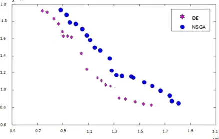
This index obtains all Pareto solutions by each algorithm altogether and then conducts non-dominant experiments on all answers and finally, the quality of algorithm is the percent of new Pareto solutions of that algorithm. The more the index value is, the better the algorithm performs. The experimental results are shown in Table 4 and Fig 2. The Pareto solutions indicate that DE works effective and efficient. The experimental results of represented model explain that the economic costs rise because of considering environmental issues and trying to strike a reasonable balance between two objective functions. The other advantage of this model, in comparison with basic models, is that it also determines how many machines must be bought in production and recovery centers. Although the income of selling salvaged materials is contemplated, it is not enough to cover the new increase of costs.
7. Conclusion
(M of Ta Ex α 0.7 0.8 0.9 MODE) has two algorit able 4 xperimental C 195 789627
been used a thms indicat
results solv
CO2 emissions
1586223 1508409 1437043 1399003 1347855 1325244 1309832 1358504 1299710 1298730 1289618 1284689 1038201 1052190 972887 969660 943800 903657 873570 864647 0.372
552..686
and its effic te that MOD
Fig. 1. P
ved by MOD
Objective Funct
0.646 2
cacy and eff DE properly
Pareto solut
DE and NSG
DE tion Cos 8049.5 8145.5 8200.9 9060.7 9706.2 10086. 10982. 110479 117591 122754 12987 13648 13821 15350 16638 16764 17800 17959 18627 19124 fficiency hav y works for
tion of MOD
GA-II st 58692 51389 96825 72513 2853 .4134 .8389 9.698 1.845 4.489 7.814 8.993 .219 ..644 8.191 4.259 0.414 ..800 7.476 4.580 823455
ve been com solving the
DE and NS
Q SM 0.7 0.525 0.6 0.372 0.8 0.488 0.8 0.495 0.312 0.584 0.7 0.654 0.4 0.627 0 0.431 0.5 0.826 0.7 0.987 0.8 0.551 0.997 0.605 0.5 0.502 0.793 0.7 0.458 0.9 0.680 0.467 0.7 0.525 mpared with e model. GA-II N Objecti QM CO2 emissions 1656743 795 1637654 646 1568433 800 1534524 867 1464573 1 1432376 1 1400323 727 1398543 433 1349710 0. 1348730 597 1328574 737 1305432 835 1243231 1 1137886 1 1116457 595 1075656 1 1035654 750 996754 965 935785 1 885744 795 h NSGA-II. NSGA II ive Function Cost s 10685.453 11453.478 11685.447 11947.455 12123.896 122862.414 126832.839 12896.345 13197.554 13567.674 13827.974 15175.536 15864.485 16007.872 16498.490 16917.268 18042.829 18859.999 19395.102 19802.674 20453.024
. The results
References
Ambrosino, D., & Scutella, M. G. (2005). Distribution Network Design: New Problems and Related Models. European Journal of Operational Research, 165(3), 610-624.
Baghalian, A., Rezapour, S., & Zanjirani Farahani, R. (2013). Robust supply chain network design with service level against disruptions and demand uncertainties: A real-life case. European Journal of Operational Research, 227(1), 199-215.
Barros, A. I., Dekker, R., & Scholten, V. (1998). A two-level network for recycling sand: a case study.
European Journal of Operational Research, 110(2), 199-214.
Drezner, Z., & Wesolowsky, G. O. (2003). Network design: selection and design of links and facility location. Transportation Research, 37(3), 241-256.
Du, F., & Evans, G. W. (2008). A bi-objective reverse logistics network analysis for post-sale service.
Computers & Operations Research, 35(8), 2617–2634.
El-Sayed, M., Afia, N., & El-Kharbotly, A. (2010). A stochastic model for forward_reverse logistics network design under risk. Computers & Industrial Engineering, 58(3), 423–431.
Fleischmann, M., Beullens, P., Bloemhof-ruwaard, J. M., & Wassenhove, L. (2001). The impact of product recovery on logistics network design. Production and Operations Management, 10(2), 156–
173.
Fleischmann, M., Bloemhof-Ruwaard, J., Dekker, R., van der Laan, E., van Nunen, J. A. E. E., & van Wassenhove, L. (1997). Quantitative models for reverse logistics: a review. European Journal of Operational Research, 103(1), 1-17.
Hinojosa, Y., Kalcsics, J., Nickel, S., Puerto, J., & Velten, S. (2008). Dynamic supply chain design with inventory. Computers & Operations Research, 35(2), 373-391.
Hugo, A., & Pistikopoulos, E. N. (2005). Environmentally conscious long-range planning and design of supply chain networks. Journal of Cleaner Production, 13(15), 1471–1491.
Hwang, C. L., & Masud, A. (1979). Multiple Objective Decision Making. Methods and Applications: A State of the Art Survey. Lecture Notes in Economics and Mathematical Systems, 164,
Springer-Verlag, Berlin.
Ilgin, M. A., Surendra, M., & Gupta, S. M. (2010). Environmentally conscious manufacturing and product recovery (ECMPRO): a review of the state of the art. Journal of Environmental
Management, 91(3), 563–591.
Jabal Ameli, M. S., Azad, N., & Rastpour, A. (2009). Designing a Supply Chain Network Model with Uncertain Demand and Lead Times. Journal of Uncertain Systems, 3(2), 123-130.
Jayaraman, V., Guige Jr., V. D. R., & Srivastava, R. (1999). A closed-loop logistics model for manufacturing. The Journal of the Operational Research Society, 50(5), 497–508.
Jayaraman, V., Patterson, R. A., & Rolland, E. (2003). The design of reverse distribution networks: models and solution procedures. European Journal of Operational Research, 150(1), 128–149.
Jiménez, M. (1996). Ranking fuzzy numbers through the comparison of its expected intervals.
International Journal of Uncertainty, Fuzziness and Knowledge-Based Systems, 4(4), 379-388.
Klibi, W., Martel, A., & Guitouni, A. (2010). The design of robust value-creating supply chain networks: a critical review. European Journal of Operational Research, 203(2), 283-293.
Ko, H. J., & Evans, G. W. (2007). A genetic-based heuristic for the dynamic integrated forward/reverse logistics network for 3PLs. Computers & Operations Research, 34(2), 346–366.
Krikke, H. R., Van Harten, A., & Schuur, P. C. (1999). Reverse logistic network re-design for copiers.
OR Spektrum, 21(3), 381–409.
Lee, D., & Dong, M. (2007). A heuristic approach to logistics network design for end-of-lease computer products recovery. Transportation ResearchPart E: Logistics and Transportation Review,
44(3), 455–474.
Listes O., & Dekker, R. (2005). A stochastic approach to a case study for product recovery network design. European Journal of Operational Research, 160(1), 268–287.
Lu, Z., & Bostel, N. (2007). A facility location model for logistics systems including reverse flows: the case of remanufacturing activities. Computers & Operations Research, 34(2), 299–323.
Melkote, S., & Daskin, M. S. (2001). Capacitated facility location/network design problem. European Journal of Operation Research, 129(3), 481-495.
Min, H., Ko, C. S., & Ko, H. J. (2006). The spatial and temporal consolidation of returned products in a closed-loop supply chain network. Computers & Industrial Engineering, 51(2), 309–320.
Ozdemir, D., Yucesan, E., & Herer, Y. T. (2006). Multi-location transshipment problem with capacitated transportation. European Journal of Operational Research, 175(1), 602-621.
Pati, R., Vrat, P., & Kumar, P. (2008). A goal programming model for paper recycling system. Omega,
36(3), 405–417.
Pirkul, H., & Jayaraman, V. (1998). A multi-commodity, Multi-Plant, Capacitated Facility Location Problem: Formulation and Efficient Heuristic Solution. Computers and Operational Research,
25(10), 869-878.
Pishvaee, M. S., Farahani, R. Z., & Dullaert, W. (2010). A memetic algorithm for bi-objective integrated forward/reverse logistics network design. Computers & Operations Research, 37(6),
1100–1112.
Pishvaee, M. S., Jolai, F., & Razmi, J. (2009). A stochastic optimization model for integrated forward/reverse logistics network design. Journal of Manufacturing Systems, 28(4), 107–114.
Pishvaee, M. S., Rabbani, M., & Torabi, S. A. (2011). A robust optimization approach to closed-loop supply chain network design under uncertainty. Applied Mathematical Modelling, 35(2), 637-649.
Pishvaee, M. S., & Razmi, J. (2012). Environmental supply chain network design using multi-objective fuzzy mathematical programming. Applied Mathematical Modelling, 36(8), 3433-3446.
Pishvaee, M. S., & Torabi, S. A. (2010). A possibilistic programming approach for closed-loop supply chain network design under uncertainty. Fuzzy Sets and Systems, 161(20), 2668-2683.
Qin, Y., & Jin, M. (2009). Optimal Model and Algorithm for Multi-Commodity Logistics Network Design Considering Stochastic Demand and Inventory Control Original Research Article. Systems Engineering-Theory & Practice, 29(4), 176-183.
Quariguasi Frota Neto, J., Bloemhof-Ruwaard, J. M., van Nunen, J. A. E .E., & van Heck, E. (2008). Designing and evaluating sustainable logistics networks. International Journal of Production Economics, 111(2), 195–208.
Quariguasi Frota Neto, J., Walther, G., Bloemhof, J., van Nunen, J. A. E. E., & Spengler, T. (2009). A methodology for assessing eco-efficiency in logistics networks. European Journal of Operational Research, 193(3), 670–682.
Salema, M. I. G., Barbosa-Povoa, A. P., & Novais, A. Q. (2007). An optimization model for the design of a capacitated multi-product reverse logistics network with uncertainty. European Journal of Operational Research, 179(3), 1063–1077.
Sawik, T. (2011). Supplier selection in make-to-order environment with risks. Mathematical and Computer Modelling, 53(9), 1670-1679.
Shaw, K., Shankar, R., Yadav, S. S., & Thakur, L. S. (2012). Supplier selection using fuzzy AHP and fuzzy multi-objective linear programming for developing low carbon supply chain. Expert Systems with Applications, 39(9), 8182-8192.
Syam, S. S. (2002). A model and methodologies for the location problem with logistical components.
Computers and Operations Research, 29(9), 1173-1193.
Thanh, P. N., Bostel, N., & Peton, O. (2008). A dynamic model for facility location in the design of complex supply chains. International Journal of Production Economics, 113(2), 678-693.
Wang, H. F., & Hsu, H. W. (2010a). Resolution of an uncertain closed-loop logistics model: An application to fuzzy linear programs with risk analysis. Journal of Environmental Management,
Wang, H. F., & Hsu, H. W. (2010b). A closed-loop logistic model with a spanning-tree based genetic algorithm. Computers & Operations Research, 37(2), 376–389.
Yager, R. R. (1981). A procedure for ordering fuzzy subsets of the unit interval. Information Sciences,