This PDF is a selection from an out-of-print volume from the National Bureau
of Economic Research
Volume Title: Behavioral Simulation Methods in Tax Policy Analysis
Volume Author/Editor: Martin Feldstein, ed.
Volume Publisher: University of Chicago Press
Volume ISBN: 0-226-24084-3
Volume URL: http://www.nber.org/books/feld83-2
Publication Date: 1983
Chapter Title: Tax Reform and Corporate Investment: A Microeconometric
Simulation Study
Chapter Author: Michael Salinger, Lawrence H. Summers
Chapter URL: http://www.nber.org/chapters/c7711
8
Tax Reform and
Corporate Investment:
A
Microeconometric
Simulation Study
Michael A. Salinger and Lawrence H. Summers
This paper develops a methodology for simulating the effects of alterna- tive corporate tax reforms on the stock market valuation and investment plans of individual firms. The methods are applied to estimate the effects of alternative corporate tax reforms on the thirty Dow Jones companies. The estimates are all based on extensions of Tobin’s q theory of invest- ment to take account of the effects of tax policy. As well as providing the basis for the estimates of the effects of tax policy, the results here provide strong microeconometric support for the q theory of investment. The q theory approach provides a superior method for estimating the effects of investment incentives because it recognizes the effects of changes in the cost of capital on the desired level of output.
A central concern in the design of tax policy is the avoidance of windfall gains or losses. This concern is closely related to the goal of providing incentives only at the margin. A crucial virtue of the q approach em- ployed here is that it provides a clear delineation of the impact of tax policies on the market value of existing capital as well as of new capital. It thus allows an examination of the incidence of tax changes on the holders of different assets. This represents an important extension of the inci- dence concepts usually used in public finance, which focus only on the rate of return on capital with no consideration of the wealth effects caused by short-run changes in its relative price.
The interaction of inflation and the corporate tax system has received widespread attention in recent years. As is by now well understood, inflation affects the corporate tax system in three important ways. His- toric cost depreciation and firms’ reluctance to use LIFO inventory accounting cause inflation to raise the tax burden on corporate capital. Michael A . Salinger and Lawrence H. Summers are with the Massachusetts Institute of Technology and the National Bureau of Economic Research.
248 Michael A. Salinger/Lawrence H. Summers
This is offset by the deductibility of nominal rather than real interest payments. While the impact of these interactions of inflation and the tax system on aggregate investment and stock market valuation has been discussed extensively, their effect on the behavior of individual firms has been little studied. Even if indexing the tax system had little effect on the level of aggregate investment or the stock market, the results in this paper suggest that it would have a large impact on the composition of invest- ment among firms. Full indexing of the corporate tax system, for exam- ple, would raise the Dow Jones average by about 8 % . The effects of the investment experience of individual firms would vary substantially.
The first section of the paper outlines the q theory of investment that provides the basis for the simulations reported in this paper. The analysis draws on the work of Hayashi (1982) and Abel(l979) in linking the Tobin q approach to investment with the firm’s problem of determining an optimal investment path in the presence of adjustment costs. In particu- lar, it shows how an investment equation relating the level of investment to tax-adjusted q can be used to infer the shape of a firm’s adjustment cost function. The q theory provides an improved basis for estimating the effects of tax reform on investment because the process of adjustment is modeled explicitly.
The estimation of q investment equations for the thirty Dow Jones companies is discussed in the second section. These estimates require the estimation of a time series of tax-adjusted q for each company. These are developed using Compustat data. The time series estimates are quite supportive of the q theory. The data confirm the importance of the tax adjustments to q suggested by the theory.
In the third section, the impact of alternative tax returns on q and investment is examined. This requires calculating the present value of the expected change in revenue which would result from alternative reforms. It is also possible to calculate the impact of these policies on the market value of individual firms’ equity. The results suggest that some reforms could have potent effects. Complete indexing would raise the Dow Jones average by an estimated 7.6%. The variance among companies is sub- stantial, with the effect ranging from - 13% for Sears to 20% for Amer- ican Brands.
The fourth section combines the results of the preceding sections to provide evidence on the response of investment to indexing the tax system and to various reforms. The results suggest that, because adjust- ment costs are very large, tax reforms are likely to have a much larger impact on long-run capital intensity than on investment in the short run. The results of the q theory approach are contrasted with those obtained using other methods.
A fifth (and final) section reviews some limitations of the analysis and suggests directions for future research.
249 Tax Reform and Corporate Investment
8.1
This section describes the procedure developed in Summers (19814 for using investment equations involving Tobin’s q as a basis for estimat- ing the impact of tax policies on both investment and the stock market. Here the focus is on the investment decisions of individual firms. The essential insight underlying Tobin’s theory is that in a taxless world, firms will invest so long as each dollar spent purchasing capital raises the market value of the firm by more than one dollar. Tobin goes on to assume that as a good approximation the market value of an additional unit of capital equals the average market value of the existing capital stock. That is, the value of the marginal “q” on an additional dollar of investment is well proxied by average q , which is the ratio of the market value of the capital stock to its replacement cost. It is natural then to assume that the rate of investment is an increasing function of the marginal return to investment as proxied by q.
An approach of this type has several virtues relative to other standard approaches to explaining investment. Perhaps most important, the q
theory approach is supply oriented. In the formulation presented below, firms make output and capital intensity decisions simultaneously. This captures the essence of an important channel through which investment stimuli are supposed to work. By reducing the cost of one factor of production, firms are encouraged to supply more output. This channel is obscured in most of the standard econometric approaches to investment decision making, in which the level of output is taken as predetermined. In this section, we show that the q theory of investment can be derived from the assumption that firms face adjustment costs and make invest- ment decisions optimally with the objective of maximizing market value. Output along with investment is treated as a choice variable.
A second virtue of the q theory approach is that it can be used to evaluate a wider menu of policy proposals than standard methods. Almost all of the empirical literature on tax policy and investment ne- glects entirely taxes levied at the personal level. These are difficult to introduce into investment equations of the flexible accelerator type. Since they d o affect stock market values, they are easily handled by the q theory approach. In addition, because the q theory is derivable directly from the assumption of intertemporal optimization, it can be used to evaluate the effects of policy announcements and temporary policies. The approach is forward looking and so can be used to study the effects of future policies on current investment. As Robert Lucas has emphasized, standard econometric investment equations cannot be used to predict the effects of any fundamental changes in policy.’ The approach developed
Taxes in a q Theory of Investment
1. This criticism applies at two levels. First, most standard approaches of the type used in policy evaluation exercises d o not include any forward looking variables. Thus there is no
250 Michael A. Salinger/Lawrence H. Summers
here is immune from this criticism because the only parameters which are estimated are technological and do not depend on the policy rule.
In what follows, the behavior of a representative, competitive firm seeking to maximize the market value of its equity is considered. We begin by examining how individuals value corporate stock and then turn to the firm’s decision problem. Throughout, it is assumed that firms neither issue new equity nor repurchase existing shares.* Hence share prices are proportional to the outstanding value of a firm’s equity. We assume that equity holders require a fixed real after-tax return p in order to induce them to hold the outstanding equity. The approach here is partial equilibrium in that the required rate of return is assumed to be unaffected by changes in tax policy. While this assumption is obviously appropriate for an individual firm, its relevance to an economy-wide tax change is less clear. However, Summers (1981a, b ) argues that any effects of tax reforms on the required rate of return are likely to be minor and of ambiguous sign. The required return p is the sum of the capital gains and dividends net of tax. It follows that
(1) (p
+
IT)K
= (1 - c)k+
(1 - OD)Div ,where c represents the effective accrual rate of taxation on capital gains,’
O D the tax rate on dividends, and IT the rate of inflation. Differences in the tax rates faced by different investors are ignored. To solve this differen- tial equation it is necessary to impose a transversality condition. We do this by requiring that at time t
This condition precludes the possibility of an explosive solution to (1). With the transversality condition satisfied and the assumption of per- fect foresight, the solution to (1) becomes
(3) 1 - c - O D Div exp
[
-js*
‘
1 - c du] dsway to use them to contemplate the effect of an announced change in policy. Implicitly, they assume that all tax parameters are expected to remain permanently constant. Second, because expected tax changes are an important feature of the historic experience, the equations are misspecified so that parameter estimates are unlikely to be reliable. The substantial importance of these problems is demonstrated by the simulations below.
2. Under the conditions described below, firms would never want to issue new equity. Legal restrictions severely limit firms’ ability to repurchase their own shares. A discussion of these restrictions and the limitations of other mechanisms which might seem to be func- tionally equivalent to repurchasing shares is contained in Auerbach (1979). For the issues considered here the assumption that shares are not repurchased is not likely to have important effects.
3. This corresponds to the statutory rate adjusted for deferral and the lack of construc- tive realization at death.
251 Tax Reform a n d C o r p o r a t e Investment
In the steady state, where taxes, the price level, and dividends are held constant, this expression reduces to
(4) (1 - OD)Div
P V =
In this case capital gains taxes do not matter because there are no capital gains. More generally, as in (3), capital gains taxes raise the discount rate on future dividends as well as affect the valuation of current dividends. Note that equation (3) implies that because of dividend taxes an extra dollar of promised dividends raises share valuation only by (1 - O D ) .
The firm seeks to choose an investment and financial policy to maxi- mize (3) subject to the constraints it faces. It is constrained by its initial capital stock and by a requirement that sources equal uses of funds. It will also be necessary to assume that credit market constraints do not permit the firm to finance more than a fraction of its investment with debt.4 This can be thought of as a measure of the firm’s debt capacity. In the model presented below, the firm will always choose to borrow as much as possible; we assume that a share b of all new investment comes from debt issues and the remainder is financed through retained earnings. Finally, the firm cannot change its capital stock costlessly. The cost of installing extra capital is assumed to rise with the rate of capital accumulation. For convenience, it is assumed that the cost function is convex and ho- mogeneous in investment and capital. Under these conditions dividends may be derived as after-tax profits less investment expenses.s That is, ( 5 ) Div = [ p F ( K , L ) -
w L
- p b i K ] ( l - T ) - [ l - ITC - b+
(1 - ~ ) + ] p l + T D+
p b K ( n - 6 R ) ,where K and L refer to factor inputs,p is the overall price level, F ( K , L ) is the production function, w is the wage rate, i is the nominal interest rate, T is the corporate tax rate, ITC is the investment tax credit,
4
is the adjustment cost function, I represents investment, 6R is the real rate of depreciaton,
and D represents the value of currently allowable deprecia- tion allowances. It has been assumed that adjustment costs are expensed and ineligible for the investment tax credit.The tax law is assumed to allow for exponential depreciation at a rate that may differ from
aR
but to be based on historical cost. This implies that4. This is acrude way of modeling the effects of bankruptcy costs on the firm’s choice of a debt-equity ratio. As noted below, the assumption of a constant debt-capital ratio is a fairly good representation of recent American experience. McDonald (1980) treats the choice of financial policy in more detail.
5. The assumption here is that all marginal equity finance comes from retained earnings. This follows from the assumption made earlier of a constant number of shares. It accounts
for some of the apparently paradoxical results described below. The last term reflects the net receipts from new debt issues (withdrawals) necessary to maintain the debt-capital ratio as the capital stock depreciates and the price level rises.
252 Michael A. Salinger/Lawrence H. Summers
(6)
Combining equations (3) and ( 5 ) , making use of (6), and rearranging yield an expression for the value of a firm's equity at time t:
(7) 0, = c6*puZuexp[ - ST(s - u ) ] du . = Jm[ [ p F ( K , L ) - W L - p b K i ] ( l - T ) - [ l - ITC - Z , - b
+
( 1 - T ) + ] p l + p b K ( n - 8)] ( l - '")FS ds + B,.
( 1 - c)PrAll the tax parameters can be arbitrary functions of time. For ease of exposition the following symbols have been introduced:
s p+7T
ps = exp
[
-j
O - d u ] 1 - CCD
2, = ~ 6 ~ e x p [ - 6T(u - s ) ] h du
.
CLS
These rather formidable expressions have simple interpretations. B, rep- resents the present value of depreciation allowances on existing capital. 2, is the present value, evaluated at the time of the investment, on a dollar of new investment. In maximizing (7) the firm can ignore B,, since it is independent of any future decisions. The constraint faced by the firm in maximizing (7) is that capital accumulation equals net investment: (9) K , =
Zs
- sRK,.
The first-order conditions for optimality are6
6. Assuming that adjustment expenses were treated as investment under the tax law would not importantly alter the results. If these costs are taken to represent managerial effort, or as interference with concurrent production, the assumption in the text is appropri- ate. Similar conditions differing because of assumptions about taxation have been derived by Hayashi (1981) and Abel (1982).
253 Tax Reform and Corporate Investment
(1 - 0”) (1 - c) (1 - T)+’
+
b ( n - S”)]Equation (lob) characterizes the investment function. It implicitly de- fines a function linking investment to the shadow price of capital Alp, and the tax parameters. The condition for zero investment is that
- - A - (’ -
e”)
[l - ITC - 2, - b ].
Pf (1 -
4
This result can be characterized in intuitive terms. It implies that the shadow price of additional capital goods is equated to their marginal cost in after-tax dollars. Equation (11) implies that there will be investment even if the shadow price of new capital goods is less than 1. This is because taxes and debt finance reduce the effective price of new capital goods.
Equation (lob) is of no operational significance as a theory of invest- ment unless an observable counterpart to the shadow price Alp, can be developed. Hayashi (1982) has shown in a similar model with a less elaborate tax system how the shadow price is linked to the market valuation of existing capital. The derivation below follows his very closely. Equation (7) implies that
Pt Kt
- (1 - ITC - 2, - b
+
(1 - T)+)Z Kusing the definition of p. The first-order conditions (10) imply that equation (12) can be rewritten
254 Michael A. Salinger/Lawrence H. Summers
Now, using the first-order condition for
A,
it can be seen thatx exp
[
-S(P.--
n--+
I S R ) d u ]l - c K
A
Pt
d s = - ’ .
The shadow price of additional capital may thus be expressed as a function of the firm’s market value. The term B, is subtracted from market value since the depreciation allowances the firm will receive on existing capital provide no inducement to further investment. Substitut- ing equation (14) in equation (lob) yields an investment function express- ible entirely in terms of observables:
- 1
+
b+
ITC+
Z ( V - B ) ( 1 - c ) pK(1 - O D ) (1 - T ) - - - I - K + g R = h K Kwhere h( ) = (+
+
(I/K) +‘) -’.
Equation (15) is a structural investmentfunction relating investment and stock market valuation.
For simplicity we postulate that up to some level of I / K , adjustment is costless. Above that level, marginal adjustment costs rise linearly with investment. That is, total adjustment costs are
= O
It follows that the function +( ) is given by
which is homogeneous in I and K as required. This implies that the investment function (15) can be written as
I 1
- = h(Q) =
K
+
-P
Q ,255 Tax Reform and Corporate Investment
By estimating equation (18) the parameters of the adjustment cost func- tion +( ) can be inferred. This is the approach taken in the next section.
Before turning to the data, it is necessary to highlight the restrictive- ness of the assumptions under which the stock market provides a proxy for the marginal q which drives investment decisions. The crucial assump- tion in the preceding derivation is that capital is both malleable and homogeneous. Only with this technological assumption does the market value of existing capital provide a proxy for the increment to market value arising from new investment. The assumption made here is incon- sistent with putty-clay formulations in which existing capital can only be used in fixed proportions while new capital is malleable. It is also incon- sistent with the view that the recent energy shocks have reduced the market value of existing energy-intensive capital but raised the incentive to invest in new energy-conserving capital.
A second restrictive assumption is that firms produce with constant returns to scale and earn no rents. If firms earn rents because of decreas- ing returns, intangible investments, or market power, these will be reflected in their market value and so measured q will not be a satisfactory proxy for the return to investment.
While these limitations are severe, they are in no way unique to the q
theoretic approach to investment. Exactly the same issues arise in con- nection with variants on the flexible accelerator approach.
8.2 Construction of the Tax-adjusted Q Variable
This section presents estimates of the Q investment equations which provide the basis for an estimate of the impact of tax policy. With the early exception of Grunfeld (1960), almost all the empirical work using q
has focused on aggregate or industry investment. Little or no account has been taken of tax effects. The construction of the necessary data is described in the appendix. The equations were estimated for the thirty Dow Jones companies.
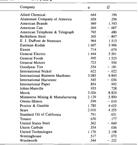
In table 8.1, estimates of Tobin's q ratio of the market value of the firm to the replacement cost of its capital stock are displayed along with the tax-adjusted variant of Q for the companies included in the sample. Note that Q is the shadow price of capital less its acquisition cost. It is therefore comparable to q - 1 rather than q . The magnitudes of the estimates appear plausible. Moreover, companies whose prospects look dim, such as the steel companies, have low values of q whereas companies with rapid growth prospects, such as IBM, have high values of q . In all
256 Michael A. Salinger/Lawrence H. Summers
Table 8.1 1978 y and Q
Company Y Q
Allied Chemical
Aluminum Company of America American Brands
American Can
American Telephone & Telegraph Bethlehem Steel E . I. DuPont de Nemours Eastman Kodak Exxon General Electric General Foods General Motors Goodyear Tire International Nickel
International Business Machines International Harvester International Paper Johns-Manville Merck
Minnesota Mining & Manufacturing Owens-Illinois
Proctor & Gamble Sears
Standard Oil of California Texaco
United States Steel Union Carbide United Technologies Westinghouse Woolworth ,644 .658 ,989 ,569 ,765 .303 .964 1.607 ,714 1.444 ,995 ,723 ,554 ,622 3.083 ,545 ,854 ,933 3.026 2.129 ,599 1.783 2.010 ,791 ,670 ,362 .554 1.170 ,517 ,544 .196 ,296 1.543 - ,007 ,480 1.513 3.906 .674 3.501 1 .S23 ,934
-
,181 - ,022 9.845 - ,034 ,992 ,728 8.829 5.850-
,010 4.625 4.255 ,631 ,177 - ,660 ,036 2.198 .072 - .222-
,807likelihood, the high values of q for some companies also reflect the market’s valuation of intangible assets. Lindenberg and Ross (1981) estimated q in a fashion similar to the estimates in this paper. They report eighteen year averages of q for each company. The correlation between the two sets of estimates of eighteen year averages of q for the twenty-five firms common to both samples is 0.953. On average, however, our estimates of q tend to be higher than theirs. We assume that capital depreciates faster than they do. Their calculations of capital-augmenting technical change only partially offset the difference in the depreciation rates. In estimating q , one needs to make many arbitrary assumptions. The high correlation between the two studies suggests that these assump- tions have more of an effect on the level than on the variations in q .
Theory, failing to take account of taxes, suggests that firms should not invest when q is less than 1. This is the case for most of the firms in the sample. Only for a much smaller fraction of the sample is the tax-adjusted
257 Tax Reform and Corporate Investment
mcasure Q less than zero. The difference is due in large part to the fact that the Q measure takes account of the effects of dividend taxes, which reduce the opportunity cost of corporate retentions. Note, however, that even using this concept, eight companies appear to have no incentive to invest. The reason that these companies actually invest almost certainly involves the failure of the assumption made here that capital is homogeneous and malleable. In a world of heterogeneous capital, even firms with very low market values will find some investment worthwhile.
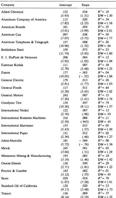
Estimates of equation (18) for the thirty companies are shown in table 8.2. The equations are all estimated using ordinary least squares. Because the estimates of Q are likely to be less reliable for the earlier years in the sample, we used only the last fifteen observations on each company. Some of the equations d o exhibit serial correlation. Rao and Griliches (1969) show that when the error process is first-order autoregressive and the autocorrelation coefficient is relatively high (generally 0.4 or greater), the GLS transformation can improve efficiency even in small samples. If the error process is of higher order, then simply doing a first-order autoregressive transformation can reduce the efficiency of the estimator. With only fifteen data points, making higher-order autocor- relation corrections is not likely to improve efficiency, so we chose not to make any autoregressive transformations. When there is positive serial correlation, however, the f statistics for the OLS estimates will be over- stated if we assume that the errors are white noise. Thus the t statistics reported are based on the assumption that the errors follow a first-order autoregressive process.
The results support the Q theory. In twenty-eight of the thirty regres- sions, the estimated slope coefficient is positive. Nearly half of the estimates are statistically significant. The low R 2 values indicate, how- ever, that much of what affects investment decisions is not captured by the Q variable. The bottom rows of the table report estimates of the equations pooling the company data. Regardless of whether allowance is made for company-specific effects, the coefficient of Q is highly signifi- cant. If different firms have the same adjustment cost functions, then both the intercept and slope will be equal across firms. Because we do not d o the GLS transformation, we cannot do an F test of this hypothesis. Instead, we d o a
x2
test, which overwhelmingly rejects the null hypothe- ses that both parameters are equal across firms. We also test for the equality of just the slopes and just the intercepts. In both cases, we reject the null hypothesis.’7. To do a xz test, we run the following regression:
= a o
+
a l Q+
a,FRMDUMl+ ..
.+
a,,FRMDUM29+
a31 FRMDUMl x Q+
. . . + a,,FRMDUM29 x Q ,I
RNPPE
+
RLINV258 Michael A. Salinger/Lawrence H. Summers
Table 8.2 Investment Equations Using Tax-adjusted Q
Company Intercept Slope
Allied Chemical
Aluminum Company of America American Brands
American Can
American Telephone & Telegraph Bethlehem Steel E. I. DuPont de Nemours Eastman Kodak Exxon General Electric General Foods General Motors Goodyear Tire International Nickel
International Business Machines International Harvester International Paper Johns-Manville Merck
Minnesota Mining & Manufacturing Owens-Illinois
Proctor & Gamble Sears
Standard Oil of California Texaco ,152 ,115 (7.82) ,101 (3.01) ,097 (7.07) .157 (10.96) ,150 (1 1.74) .206 (5.92) .111 (2.79) .177 (10.05) .179 (2.81) .117 .242 (7.26) .134 (10.56) .122 (2.76) .316 (2.59) .153 .151 (2.39) .181 (5.72) .245 (3.04) ,193 (3.19) .130 (2.71) .163 (3.12) .029 (1.07) .120 (9.17) ,136 (8.14) (5.93) (5.39) (5.43) ,018 (1.31) .020 (2.23) ,059 (3.99) .038 (3.75) ,008 (1.32) .073 (3.45) .004 (1.02) .007 (3.48)
-
,003 .013 (1.77) ,011 .007 (1.41) ,037 (6.11) ,007 ,006 ,015 .012-
,009 ( - .76) .001 ,005 (1.46) ,030 (1.81) ,002 ,016 (7.28) .020 (3.48) ,009 (2.19) ( - .55) (3.45) (.96) ( ,945) ( 5 7 ) (.46) ( 5 1 ) (.33) R 2 = . 1 9 DW=1.30 R 2 = . 3 4 DW=1.56 R 2 = .55 DW=2.01 R 2 = .56 DW = 1.77 R 2 = .26 DW=.64 R 2 = .53 D W = 1.60 R 2 = . 1 2 DW=1.09 R 2 = .58 DW=1.25 R 2 = . 0 4 DW=1.06 R 2 = .26 D W = 1.03 R 2 = .64 D W = 1.02 R 2 = .15 DW=1.74 R 2 = .74 DW = 1.57 R 2 = .13 DW=.93 R 2 = . l l DW=.45 R 2 = .05 DW=1.00 R 2 = .02 DW=1.27 R 2 = .06 DW = 1.36 R 2 = .03 DW=1.29 R 2 = .18 DW=1.42 R 2 = .29 DW = 1.22 R 2 = .01 DW = .95 R 2 = .79 DW=1.91 R 2 = .53 DW=1.73 R 2 = .37 D W = 1.35259 Tax Reform and Corporate Investment
Table 8.2 (cont.)
Company Intercept Slope
United States Steel .090
(5.28) Union Carbide ,169 United Technologies .114 (2.25) Westinghouse .113 (4.30) Woolworth ,181 (7.31) All companies with common intercept .166
(21.09) All companies with different intercepts . . .
(7.37) .010 R 2 = .04 ( 3 5 ) DW=.69 ,009 R 2 = .10 (.51) DW=1.10 .068 R 2 = .56 (3.18) DW=1.15 ,022 R 2 = .57 (3.24) DW = 1.05 .013 R 2 = .25 (1.41) DW=.68 ,004 R 2 = 2 8 .006 R 2 = . 5 4 (4.77) (4.32)
The theory of investment developed in the preceding section implies that lagged values of q should not have any effect on current investment. It takes no account of delivery lags or lags in implementing investment plans. This is a potentially serious difficulty. The equations in table 8.2 were therefore reestimated including lagged values. While this improved their explanatory power a little bit, lagged Q was rarely significant, so these results are not reported here.
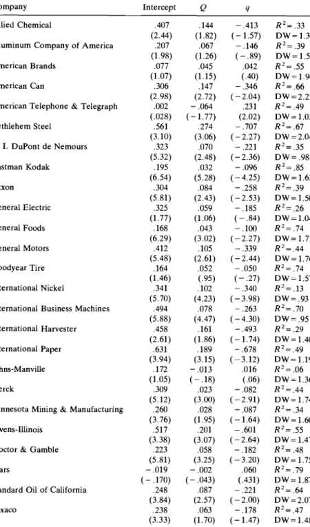
In table 8.3, the relative explanatory power of Q and q is contrasted. If equation (18) were the true investment function, then the coefficient on Q would be positive and significant and the coefficient on q would be insignificant. With only three exceptions, the coefficient of Q is positive; in over half the regressions, it is significant. Nearly all of the coefficients of q are negative, and nearly half are significant. This is not surprising. Because capital is not homogeneous and the stock market is extremely volatile, one would expect the stock market component of q to be a very noisy signal of the marginal return on incremental investment. The tax-adjustment parts of the Q series are much less subject to error. It is therefore reasonable to expect that their effect would be greater than that of the stock market. This is reflected in the negative coefficients on q . This point underscores the importance of making tax adjustments in studying the relation between investment and q.R
matrix of the regression. Let V be the lower right-hand 58 x 58 submatrix of V. Let a be the column vector composed of u2 to a5y. Under the null hypothesis that the adjustment cost functions are identical, u ' ( V ) -
'&,&.
The test statistic is 357.8. The statistics for the tests that just the intercepts and just the slopes are equal are, respectively, 95.5 and 120.8. Notice that our estimate of the covariance matrix asymptotically approaches the true covariance matrix only as f+=. Even though the pooled regression has 450 data points, Tis still 15, so the asymptotic distribution of the test is unlikely to hold.8. If we had a larger sample, we could handle the errors in variables with an instrumental variables procedure. The tax rates are appropriate instruments because they are measured
260 Michael A. Salinger/Lawrence H. Summers
Table 8.3 Investment Equations Using Q and q
Company Intercept Q 9
Allied Chemical
Aluminum Company of America American Brands
American Can
American Telephone & Telegraph
Bethlehem Steel E . I. DuPont de Nemours Eastman Kodak Exxon General Electric General Foods General Motors Goodyear Tire International Nickel
International Business Machines
International Harvester
International Paper
Johns-Manville
Merck
Minnesota Mining & Manufacturing
Owens-Illinois
Proctor & Gamble
Sears
Standard Oil of California
Texaco ,407 (2.44) ,207 (1.98) ,077 (1.07) ,306 (2.98) ,002 (.028) ,561 (3.10) ,323 (5.32) ,195 (6.54) ,304 (5.81) ,325 (1.77) .168 (6.29) ,412 (5.48) ,164 (1.46) ,341 (5.70) ,494 (5.88) ,458 (2.61) ,631 ,172 (1.05) ,309 (5.12) ,260 (3.76) S17 (3.38) ,223 (5.81) - ,019 ( - ,170) (3.94) ,248 (3.84) ,238 ,144 (1.82) ,067 (1.26) ,045 (1.15) ,147 (2.72) - ,064 ( - 1.77) ,274 (3.06) ,070 (2.48) .032 (5.28) ,084 (2.43) ,059 (1.06) .043 (3.02) ,105 (2.61) .052 .lo2 (4.23) .078 ,161 (1.86) .189 (3.15) (.95) (4.47) - .013 ( - .18) ,023 ,028 (1.95) ,201 (3.07) ,058 (3.25) - ,002 ( - ,043) ,087 (2.57) ,063 (3.00) - ,413 ( - 1.57) - .146 ( - .89) ,042 (.40) - ,346 (- 2.04) ,231 (2.02) - ,707 (-2.27) - ,221 ( - 2.36) R 2 = . 3 3 D W = 1.30 R 2 = . 3 9 DW=1.56 R'= .55 DW=1.96 R 2 = . 6 6 DW=2.22 R 2 = . 4 9 DW=1.03 R 2 = .67 D W = 2.04 R 2 = .35 DW=.98 -.096 R Z = . 8 5 -4.25) DWz1.63 -.258 R2=.39 -2.53) DW=1.50 -.185 R Z = . 2 6 (-.84) DW=1.04 -.lo0 R 2 = . 7 4 -2.27) DW=1.71 -.339 R 2 = . 4 4 ( - 2.44) - ,050 ( - .27) - ,340 (-3.98) - ,263 ( - 4.30) - ,493 ( - 1.74) - ,678 (-3.12) ,016 (.06) - .082 (-2.91) - .087 ( - 1.64) - .601 (-2.64) - .182 ( - 3.20) .060 (.431) - ,221 - '178 (- 2.00) DW = 1.76 R 2 = .74 D W = 1.57 R 2 = .13 DW=.93 R 2 = .70 DW=.95 R 2 = .29 DW=1.40 R 2 = .49 DW=1.19 R Z = .06 DW=1.36 R Z = .44 DW = 1.74 R 2 = .34 DW=1.60 R Z = .55 D W = 1.47 R Z = .48 DW=1.75 R2=.79 DW=1.87 R2= .64 DW = 2.07 R Z = .47 (3.33) (1.70) (-1.47) DW=1.48
261 Tax Reform and Corporate Investment
Table 8.3 (cont.)
Company Intercept Q 4
United States Steel .196 ,070 -.170 R2=.04
(3.91) (2.52) (-2.38) DW=.75 (1.36) (.83) (-.73) D W z l . 8 7 (1.90) (2.37) (-1.10) DW=1.34 (1.96) (.89) (-.17) DW=1.08 (3.45) (1.36) (-1.05) DW=.99 Union Carbide ,419 ,142 -.428 R Z = . 3 8 United Technologies ,239 ,122 -.195 R 2 = . 6 0 Westinghouse ,122 ,028 -.017 R 2 = . 5 7 Woolworth ,254 .052 -.132 R’z.32
All companies with common intercept .226 ,031 -0.90 R 2 = . 3 3
All companies with different intercepts . . . ,033 -.099 R2=.59 (12.08) (4.16) (-3.48)
(5.15) (-4.38)
The results obtained in this section provide quite strong microecon- ometric support for the q theory of investment. The results parallel closely those obtained in Summers’ (19814 study of aggregate invest- ment over the entire 1929-78 period. The aggregate results suggest a somewhat larger responsiveness of investment to q than is found here. This is probably because aggregation reduces some of the noise in indi- vidual firms’ q. Future progress in reconciling micro- and macroestimates of the effects of q , and in improving the explanatory power of these equations, must await the development of methods for taking account of rents and the nonhomogeneity of the capital stock.
8.3 Tax Reform and Corporate Valuation
This section assesses the impact of alternative tax reforms on corporate profitability and on share valuation. The equations estimated in the previous section provide the basis for estimating the impact of a given tax reform on a firm’s investment. In order to estimate the effect of a given tax reform on a firm’s investment, one must first calculate its effect on Q. The principal difficulty in this calculation comes in estimating the effect of the reform on V , the market value of firm equity. The procedure followed here is to estimate the impact on the market value of equity by calculating the present value of the change in tax liabilities which a reform will cause assuming that the firm’s growth is not affected by the tax change.
A proper calculation of this type would require the simultaneous estimation of the entire growth path of the firm. This path is of course precisely compared with the value and replacement cost of the firm and because they are determined exogenously. In small samples, however, instrumental variable regressions are badly biased.
262 Michael A. Salingerl Lawrence H. Summers
affected by tax reforms. Deriving the path of investment following a tax change requires the solution of a two-point boundary value problem as described in Summers (1981a). Because the response of investment to change in
Q
is estimated to be small, the approximation error involved is likely to be very small.The first step in estimating the change in market value from a tax change is estimating its effect on after-tax profits. In this paper, we consider three alternative tax reforms: indexation of the tax system to adjust for inflation, 25% acceleration of depreciation deductions, and reduction in the statutory corporate tax rate from 46 to 40%.’ It is easiest to begin by describing how the change in profits arising from the corpo- rate rate reduction was calculated.
In general, reported profits differ from taxable profits. As a result, to estimate the effect of a change in the corporate tax rate, we look at actual taxes paid. With a tax rate of 46%, taxes are given by
T = 0 . 4 6 1 ~ ~ - ITC - FTC,
where T = taxes,
IT^
= taxable profits, ITC = investment tax credit, and FTC = foreign tax credit. Reducing the corporate tax rate to 0.40 increases profits by 0 . 6 ~ ~ . We assume that all foreign taxes paid can be claimed as a credit.’O Thus we estimate the change in profits by6 46
An (tax reduction) = - (T
+
ITC+
FTC).
(19)
The change in profits from accelerating depreciation and using replace- ment cost depreciation are, respectively,
AIT (depreciation acceleration) -
-
(:
‘
E)NPLT x 0.46, AIT (replacement cost depreciation)L
= -(NPL~ - N P L ~ ) x 0.46. L
In indexing debt, we allow firms to deduct only real interest payments on the market value of the debt. Using an ARMA procedure based only on prior data, we estimate that at the beginning of 1978 the expected inflation rate over a long horizon was 0.053. We thus deduct from profits: 9. Specifically, we assume that the useful life for tax purposes is reduced by 25%. The reduction results in a 33%% increase in 6 , the depreciation rate.
10. Firms may claim foreign taxes up to the United States statutory tax rate times foreign pretax profits as a tax credit. The maximum applies to all foreign taxes paid. Thus a firm can offset taxes above the United States corporate tax rate by operating in another country with a tax rate lower than the United States’.
263 Tax Reform and Corporate Investment
(20) A.rr(debt indexation) = 0.053 x MVDEBT X 0.46.
In general, the inventory adjustment is
(21) An(inventory indexation) = 0.46 X FRFIFO
CPI x INV-1 x
-.
CPI - 1
When inventories are drawn down, however, an adjustment also has to be made for liquidated LIFO inventories. As in the estimation of real inventories, we assume that the reduction in LIFO inventories comes from goods purchased in the previous year.
To estimate the change in market value, we need to project future values for each firm's taxes, net plant, debt, and inventories. We assume that the real value of these quantities grows at the same rate. We esti- mated the growth rate of real net property, plant, and equipment from 1964 to 1978. Over that period, some of the firms had growth rates exceeding 10% per year. In general, such growth rates reflect the adjust- ment to a new equilibrium and we do not expect them to continue. Thus we average the historic growth rate with 3% to get expected future growth.
In the calculations below, it is assumed that investors expect that the rate of inflation will remain permanently at 0.053. It is assumed that potential tax reforms are permanent and unanticipated. When consider- ing, for example, the acceleration of depreciation, we assume that people did not foresee the tax law change. When the change occurs, people expect it to last forever. We assume that a real discount rate of 10% can be applied to all cash flows. This may be misleading, since the risk characteristics of depreciation allowances differ greatly from those of pretax profits.
The formula for the change in V from corporate tax rate reduction, inventory indexation, and debt indexation is
AT 1 - O D
AV=--
0 . 1 - g 1 - c '
where g is the growth rate. To reduce the effect of wide annual fluctua- tions, we use three year averages of inventories and taxes paid rather than the 1978 values. The averages are calculated in real terms and adjusted for growth.
The change in Vfrom a change in the depreciation tax law is the sum of the changes in the value of depreciation deductions on existing capital and on future additions to capital. The former is simply the change in B .
New investment at time t is given by
NI(t) = g
+
- RNPPE(0)eg',264 Michael A. SalingerILawrence H. Summers
where RNPPE represents the real value of net property, plant, and equipment. The change in the value of the depreciation deduction at time t of investment at time t is the change in Z . Thus the change in the value of depreciation deductions on all future new investment is the change in Z times the discounted stream of investment.
While most recent discussions of corporate tax reforms have focused on the likely impact on investment, issues of equity should be considered as well. Unsophisticated observers focus on the distinction between tax relief for business and for individuals. This is misleading, as corporations should be thought of as conduits. All taxes are ultimately borne by individuals in their role as labor suppliers, consumers, or suppliers of capital. The change in the value of the stock market following a tax change is a direct measure of the present value of the burdens it will impose on the suppliers of equity capital. It thus seems a natural candi- date for measuring the incidence of capital tax reforms.
In addition to examining the impact of tax policy on the functional distribution of income, it is instructive to model the effects of tax reforms on the stock market for two other reasons. First, it is widely accepted that a good tax reform should minimize windfall gains and losses. The size of the policy-induced jump in the stock market is a good measure of its windfall effect. If, as available evidence suggests, investors fail to hold diversified portfolios, then differential effects of tax reforms on different securities create windfall gains and losses.
Second, the effect of tax policy on the stock market is of concern to those sensitive to issues of vertical equity. Virtually all corporate equity is owned directly or indirectly by the very wealthy. About 75% is held directly by individuals. Of this, available evidence indicates that about 50% is held by families with incomes in the top 1% of the population. This actually understates the true concentration because much of the remainder of the stock is held by individuals with deceptively low re- ported incomes due to successful sheltering or life-cycle effects. The remaining stock is mostly held by pension funds, foreigners, and insur- ance companies. Since almost all pension plans offer defined benefits, the pension’s assets are ultimately owned not by the beneficiaries but by the shareowners in the corporations with pension liabilities. Hence this stock also should be assigned primarily to rich households. The distributional consequences of insurance company and foreign ownership are less clear. But the conclusion that any tax-induced change in profitability which shows up in the stock market redounds almost entirely to the very wealthy seems inevitable. Therefore the analysis below focuses on the effects of tax reforms on both investment and the stock market. Recent research suggests the importance of dividend clienteles. This implies that changes in the relative valuation of different firms may have large effects on the distribution of wealth.
265 Tax Reform and Corporate Investment
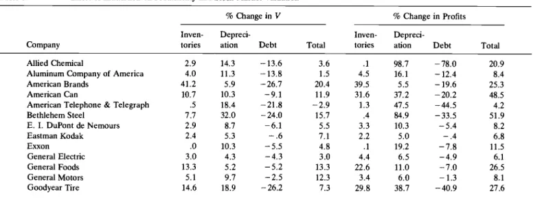
In table 8.4 the effects of indexing the tax system are considered. The relative effects of the different components of indexing vary among firms. Indexing debt has a small impact on Kodak, which is almost entirely equity financed, and a large impact on AT&T, which is largely debt financed. Inventory indexation has no effect on firms already using LIFO but a large effect on American Brands, which primarily uses FIFO. With only two exceptions, the effect of total indexation is to increase firm value, thus suggesting that the interaction of inflation and corporate taxes has at least partially contributed to the decline in the real value of the stock market. In some cases, indexation has a significantly larger impact on profits than on firm value. This phenomenon is undoubtedly a result of some firms having unusually low real profits in 1978. In making these calculations, we implicitly assume that a reduction in taxable profits is of value to the firm. The effect of total indexation on firm value ranges from - 13.3% for Sears to 20.4% for American Brands. Typically, indexation leads to an increase in firm value of between 5% and 10%.
This contradicts the results of several earlier studies (e.g. Shoven and Bulow 1975) which suggested that indexing would be approximately neutral or actually increase corporate income tax liabilities. The reason is that our calculation focuses on the long-run impact of increases in infla- tion rather than their immediate impact on the current income, which includes revaluations of outstanding long-term debt.
These calculations of the impact of indexation on stock market valua- tions implicitly assume that the market is rational with respect to infla- tion. This hypothesis is examined explicitly in Summers (1981c), who finds some evidence that at least historically the market has failed to fully recognize the effects of inflation-taxation interactions.
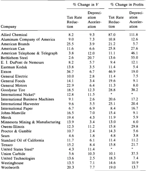
Table 8.5 considers the effect of reducing the corporate tax rate from 0.46 to 0.4 and of accelerating depreciation by 25%. O n average, the latter reform increases firm value by 7 % . Not surprisingly, the effect on capital-intensive firms is larger. The effect of a reduction in the tax rate ranges from 4.1% for Bethlehem Steel to 34.7% for Exxon. If taxable income equals real income, the tax rate reduction should increase firm value by 11%. Because the interaction of inflation and the tax system cause taxable profits to be higher than real profits, the tax rate reduction should increase firm value by more than 11%. In fact, the average increase in firm value from indexing in table 8.4 is consistent with the 13% average increase in firm value from a tax rate reduction. The variation among firms of the effect of indexing does not, however, explain the variation of the effect of the tax rate reduction. The 34.7% increase in Exxon’s value, for example, cannot be explained by the inflation-induced overstatement of profits. In 1978, Exxon’s foreign and federal taxes were 65% of its taxable income. A large portion of Exxon’s taxes were foreign. Saudi Arabia levies a large “tax” on oil extraction. It is not clear that this
Table 8.4 Effect of Indexation on Profitability and Stock Market Valuation
Company
~ ~~
% Change in V % Change in Profits
Inven- Depreci- h e n - Depreci-
tones ation Debt Total tories ation Debt Total
Allied Chemical
Aluminum Company of America American Brands
American Can
American Telephone & Telegraph Bethlehem Steel E. I. DuPont de Nemours Eastman Kodak Exxon General Electric General Foods General Motors Goodyear Tire 2.9 14.3 4.0 11.3 41.2 5.9 10.7 10.3 .5 18.4 7.7 32.0 2.9 8.7 2.4 5.3
.o
10.3 3.0 4.3 13.3 5.2 5.1 9.7 14.6 18.9 - 13.6-
13.8 -26.7 -9.1 -21.8 -24.0 -6.1 - .6 -5.5 -4.3 -5.2 -2.5 - 26.2 3.6 .1 98.7 1.5 4.5 16.1 20.4 39.5 5.5 11.9 31.6 37.2 - 2.9 1.3 47.5 15.7 .4 84.9 5.5 3.3 10.3 7.1 2.2 5.0 4.8 .1 19.2 3.0 4.4 6.5 13.3 22.6 11.0 12.3 3.4 6.0 7.3 29.8 38.7 -78.0 - 12.4 - 19.6 -20.2 -44.5 - 33.5 -5.4 - .4 -7.8 -4.9 -7.0 - 1.3 -40.9 20.9 8.4 25.3 48.5 4.2 51.9 8.2 6.8 11.5 6.1 26.5 8.1 27.6International Nickel" 25.7 18.0 -28.7 15.0
International Business Machines .8 3.8 - .2 4.4 2.1 9.1 - .6 10.6
International Harvester 16.7 8.4 - 22.6 2.5 37.2 20.4 -38.1 19.5
Johns-Manville
.o
10.9 -9.2 1.7.o
9.6 - 6.5 3.2Merck 8.9 6.6 -5.6 9.9 6.8 3.9 -3.5 7.2
Minnesota Mining & Manufacturing 7.5 5.2 - 3.5 9.2 7.2 4.7 -2.8 9.2
Owens-Illinois 7.0 17.3 - 19.5 4.8 12.1 32.2 -26.4 17.9
Proctor & Gamble 2.2 3.7 - 3.2 2.7 3.8 6.0 -4.2 5.6
Sears
.o
2.8 - 16.1 - 13.3 .4 4.5 - 17.2 - 12.2Standard Oil of California 2.0 9.4 -5.1 6.3 .8 13.6 -4.8 9.6
Texaco 4.0 13.0 - 9.3 7.7 2.2 25.3 - 12.3 15.2
United States Steel"
.o
17.8 - 16.3 1.5Union Carbide 6.1 15.8 - 15.7 6.2 .2 32.3 - 27.0 5.5 United Technologies 12.6 3.7 -3.8 12.5 17.7 6.0 - 4.7 19.0 Westinghouse 9.9 11.0 - 7.0 13.9 9.9 12.9 -5.5 17.3 Woolworth 20.7 11.7 - 17.1 15.3 21.0 13.2 - 13.7 20.5 * * * * International Paper 21.8 10.6 - 12.2 20.2 3.3 16.8 - 14.3 5.7 * * * t 'Negative profits in 1978.
268 Michael A. Salinger/Lawrence H. Summers
Table 8.5 Effect of Tax Changes on Profitability and Stock Market Valuation
% Change in V % Change in Profits
Depreci- Depreci-
Tax Rate ation Tax Rate ation Reduc- Acceler- Reduc- Acceler-
Company tion ation tion ation
Allied Chemical
Aluminum Company of America American Brands
American Can
American Telephone & Telegraph Bethlehem Steel E. I. DuPont de Nemours Eastman Kodak Exxon General Electric General Foods General Motors Goodyear Tire International Nickel”
International Business Machines International Harvester International Paper Johns-Manville Merck
Minnesota Mining & Manufacturing Owens-Illinois
Proctor & Gamble Sears
Standard Oil of California Texaco
United States Steel” Union Carbide United Technologies Westinghouse Woolworth 8.2 9.0 25.5 11.6 3.8 2.6 8.2 13.8 34.7 10.0 14.1 22.9 18.5 12.8 9.1 9.6 6.7 16.5 19.4 13.9 12.3 10.7 4.6 11.7 15.2 4.3 5.6 13.6 13.5 20.3 9.3 7.3 3.9 6.6 12.0 20.7 5.7 3.5 6.7 2.8 3.4 6.4 12.3 11.5 2.6 5.5 6.9 7.0 4.3 3.4 11.2 2.4 1.8 6.1 8.4 11.4 10.3 2.5 7.1 7.7 87.0 10.8 21.2 25.8 11.1 13.6 9.4 11.4 46.9 11.4 19.6 11.3 28.8 20.6 25.1 8.4 15.4 11.9 13.0 15.8 14.3 4.8 11.4 15.8 10.1 18.3 14.6 19.0 * * 111.8 12.6 5.7 27.6 46.1 55.0 12.1 5.4 19.0 7.5 9.1 8.0 38.2 17.2 20.4 16.7 9.1 5.9 6.0 29.8 5.6 3.8 11.2 21.7 37.5 7.4 10.9 13.7 * * ”Negative profits in 1978.
tax is an income tax, so it may not qualify for the foreign tax credit. Even if it does, the tax may be large enough to make Exxon’s tax rate on foreign profits well above 0.46. In either case, our assumption that all foreign taxes can be claimed as a credit is likely to be violated.
8.4 Tax Reforms, Q, and Investment
In this section we derive estimates of the impact of the tax reform packages considered above on firm investment. The estimates are calcu-
269 Tax Reform and Corporate Investment
lated first by using the estimates of the impact of tax changes on V displayed in tables 8.4 and 8.5 to find the estimated change in Q, and then by multiplying this figure by the coefficient on Q in the firm investment equation.
It should be stressed at the outset that these estimates are subject to very substantial error. Beyond the difficulties of inaccuracy in the data, a major limitation of the analysis is that for some firms the effect of changes in Q is estimated only with a large standard error. Moreover, the effect of tax reforms on V is estimable only approximately due to the somewhat arbitrary assumptions made about the choice of a discount and growth rate, and the neglect of the economy-wide feedback effects of increased capital accumulation. While these conclusions are, to say the least, tentative, they illustrate the potential of this methodology for a much richer analysis of the effects of tax changes.
An additional issue is posed by FIFO inventory accounting. As table 8.4 demonstrates, a substantial fraction of the gains to corporations from indexing arise from the elimination of the taxation of FIFO profits. There exist some reasons to believe that any extra taxes incurred as a result of FIFO inventory accounting do not discourage investment in plant and equipment. It is argued that the taxes are voluntary and so are unlikely to be paid if they impose a burden. In addition it is argued that taxes on inventory holdings should have no impact on the return to plant and equipment investment and so should not affect these investment decisions.
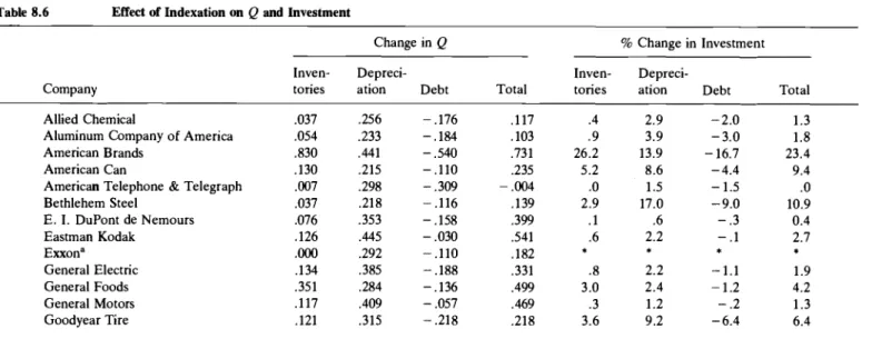
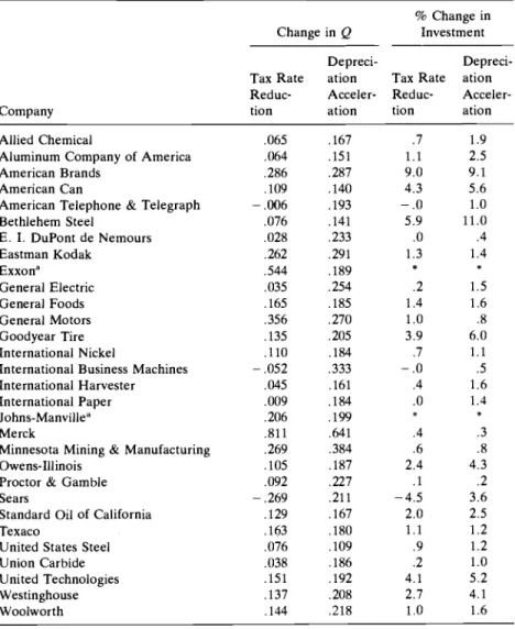
Table 8.6 presents the effects of indexation on Q and on investment. While there is considerable variation among firms, total indexation generally increases investment by less than 5 % . Table 8.7 gives the projections of how lowering the corporate tax rate and accelerating depreciation affect Q and investment. Again, the increase in investment by most of the firms is between 0% and 5%. Comparing these results with tables 8.4 and 8.5, it is clear that the tax changes have a larger impact on firm valuation than on investment.
Comparing tables 8.6 and 8.7 with tables 8.4 and 8.5, it can be seen that in the short run the costs of these changes are large compared with their benefits. In many cases, the amendments would have a much greater impact on firm value than on investment. For example, completely indexing the tax system would increase International Paper’s market value by 20.2%. At the same time, International Paper would increment its investments by only 0.6%. Similarly, a 15% growth in the value of International Nickel would stimulate additional investment of only 1.5%. While these firms are outliers, market value would increase twice as much as investment for most firms.
The large change in firm value would also have an undesirable impact on the distribution of wealth. These changes in the corporate income tax
Table 8.6 Effect of Indexation on Q and Investment
Company
Change in Q % Change in Investment
Inven- Depreci- Inven- Depreci-
tories ation Debt Total tones ation Debt Total
Allied Chemical
Aluminum Company of America
American Brands American Can
American Telephone & Telegraph Bethlehem Steel E. I. DuPont de Nemours Eastman Kodak Exxon" General Electric General Foods General Motors Goodyear Tire ,037 ,054 ,830 .130 .007 .037 .076 .126 .Ooo ,134 ,351 ,117 ,121 ,256 ,233 .441 .215 .298 .218 .353 .445 .292 ,385 ,284 .409 .31S - ,176 -.184 - .540 - .110 - .309 -.116 - .158 - .030 - ,110 - ,188 - .136 - .057 - .218 - .117 .lo3 ,731 ,235 .004 ,139 ,399 ,541 .la2 .331 .499 ,469 ,218 .4 2.9 .9 3.9 26.2 13.9 5.2 8.6 .o 1.5 2.9 17.0 .1 .6 .6 2.2
.a
2.2 3.0 2.4 .3 1.2 3.6 9.2 * * -2.0 1.3 - 3.0 1.8 - 16.7 23.4 - 4.4 9.4 - 1.5.o
-9.0 10.9 - .3 0.4 - .1 2.7 -1.1 1.9 - 1.2 4.2 - .2 1.3 -6.4 6.4 * *International Nickel
International Business Machines International Harvester International Paper Johns-Manville" Merck
Minnesota Mining & Manufacturing Owens-Illinois
Proctor & Gamble Sears
Standard Oil of California Texaco
United States Steel Union Carbide United Technologies Westinghouse Woolworth ,267 ,087 ,135 ,042 .Ooo ,853 ,514 ,076 ,128
.ooo
,040 .057 .ooo .070 .400 ,136 ,174 ,287 ,498 ,245 ,283 .308 .980 ,584 .288 ,352 ,323 ,257 ,277 ,170 ,286 ,292 .320 ,331 - ,297 - .027 - ,183 - ,239 - ,179 - ,537 - ,240 - ,210 - .184 - .651 - ,098 - .133 - ,105 - ,179 - ,120 - ,096 - ,144 ,257 ,558 ,197 ,086 .129 1.296 ,858 ,154 ,296 - ,328 .199 ,201 ,065 ,177 ,572 .360 .361 1.6 1.7 .1 .8 1.4 2.5 .3 2.1 .4 .5 1.1 1.2 1.7 6.6 .1 .4.o
5.5 .6 3.9 .4 1.8.o
1.9 .4 1.5 10.7 7.8 2.7 6.3 1.3 2.4 * * - 1.8 - .O - 1.8 - 1.8 - .3 - .5 -4.8 - .2 -11.0 - 1.5 - .9 - 1.2 - 1.0 -3.2 - 1.9 - 1.0 * 1.5 .9 2.1 .6 .6 1.8 3.5 .3 -5.5 3.0 1.3 .7 .9 15.3 7.1 2.7 *272 Michael A. Salinger/Lawrence H. Summers
Table 8.7 Effect of Tax Reforms on Q and Investment
Company
% Change in Change in Q Investment
Depreci- Depreci-
Tax Rate ation Tax Rate ation Reduc- Acceler- Reduc- Acceler-
tion ation tion ation
Allied Chemical
Aluminum Company of America American Brands
American Can
American Telephone & Telegraph Bethlehem Steel E . I. DuPont de Nemours Eastman Kodak Exxon" General Electric General Foods General Motors Goodyear Tire International Nickel
International Business Machines International Harvester International Paper Johns-Manville" Merck
Minnesota Mining & Manufacturing Owens-Illinois
Proctor & Gamble Sears
Standard Oil of California Texaco
United States Steel Union Carbide United Technologies Westinghouse Woolworth ,065 ,064 ,286 ,109 ,006 ,076 ,028 ,262 .544 ,035 ,165 .356 ,135 ,110 ,052 .045 ,009 ,206 ,811 .269 ,105 ,092 ,269 ,129 ,163 ,076 ,038 ,151 .137 ,144 ,167 ,151 ,287 ,140 ,193 .141 ,233 .291 ,189 ,254 ,185 ,270 .205 .184 ,333 ,161 ,184 ,199 ,641 .384 ,187 .227 ,211 ,167 ,180 .lo9 ,186 ,192 ,208 ,218 .7 1.1 9.0 4.3 - .O 5.9
.o
1.3 .2 1.4 1.o
3.9 .7 -.o
.4.o
.4 .6 2.4 .1 .4.5 2.0 1.1 .9 .2 4.1 2.7 1.0 * * 1.9 2.5 9.1 5.6 1.o
11.0 .4 1.4 1.5 1.6 .8 6.0 1.1 .5 1.6 1.4 .3 .8 4.3 .2 3.6 2.5 1.2 1.2 1.0 5.2 4.1 1.6 * *"Change in investment not projected when estimated coefficient of tax-adjusted Q is negative.
are being considered along with reductions in personal income taxes for people in top income brackets. Combined, these policies may cause a large shift of wealth to those who are already wealthy.
If the government's objective is to increase investment, it should implement the reforms which most directly affect the relative cost of capital. Indexing or accelerating depreciation induces more investment for a given increase in market value than do the other changes. Consider, for example, the effects of indexing inventories and depreciation for
273 Tax Reform and Corporate Investment
American Can. The two changes have a nearly equal effect on firm valuation, but depreciation indexing has almost twice the effect on invest- ment that inventory indexing does. Similarly, the tax rate reduction would increase the value of Goodyear by 20.4% while the depreciation acceleration would increase it by only 12.3%. The latter change would, however, increase Goodyear’s investment more than the former.
Investment studies that use aggregate data miss the effect of policies on the composition of investment. Yet, the results in this study suggest that the impact of tax changes would vary significantly across firms. Since these results are for a small number of firms, it is difficult to say whether most of the variation is across or within industries. Insofar as adjustment costs are part of an industry’s technology, one might expect similar results for firms in the same industry. O n the other hand, the analysis in section 8.1 assumed a competitive market structure. Especially for the Dow 30, this assumption is tenuous. It is possible that the response to a tax change could depend on a firm’s competitive position within an industry. The three chemical firms in the sample show similar responses to all the changes. In contrast, though, Bethlehem Steel’s investment is much more sensitive to tax changes than United States Steel’s. A n important exten- sion of this paper would be to explore more systematically the effect of taxes on the composition of investment.
8.5 Conclusions
This preliminary attempt to examine the impact of alternative tax reforms on the investment decisions of individual firms has yielded prom- ising results. The q theory approach has substantial predictive power at the microlevel. The econometric results suggest that explanatory power is enhanced even further when tax effects are recognized. The simulation results confirm that tax policies can have large effects on both stock market valuations and investment incentives in both the short and the long run. They also indicate that the effects of investment incentives are likely to differ very substantially across firms.
The differences arise from variations both in the magnitude of tax effects on firms’ incentives to invest and in the responsiveness of firms’ investment to changes in investment incentives. The latter are due, according to the model, to differing adjustment cost functions.
While these results are informative and encouraging, a great deal needs to be done before it will be possible to make accurate predictions of the impact of tax reforms on individual corporate o r even industry invest- ment decisions. The most important area for further investigation is the relaxation of the stringent assumptions about the homogeneity of capital and absence of rents that were made here. This will probably necessitate the addition of other variables to Q investment equations. Ultimately,
274 Michael A. Salinger/Lawrence H. Summers
work along these lines promises us a greater understanding not just of tax effects on investment but also of tax effects on the other components of a firm's net worth such as intangibles.
Appendix
The source of the data is the Compustat tapes and spans the years 1959 to 1978. To estimate tax-adjusted Q, we need estimates of the market value of equity, the market value of debt, the replacement value of inventories, the replacement value of the capital stock, and the taxable capital stock. Throughout the analysis, we tried to get these figures for the beginning of each year.
Market Value of Equity
Compustat gives the closing price of a share of stock for each company. The value of common stock at the beginning of the year is estimated as the closing value in year t - 1 times the number of shares outstanding at r - 1. The value of preferred stock is estimated by dividing preferred dividends by the Standard and Poor's preferred stock yield.
Market Value of Debt
Compustat lists the book value of both long-term and short-term debt. We assume that the market value of short-term debt equals the book value. In principle, to estimate the market value of long-term debt, we need to know the years to maturity, coupon rate, and default characteris- tics of all debt issues. Compustat does not have this information. Follow- ing Brainard, Shoven, and Weiss (1980), we assume: (1) All new issues of long-term debt have a maturity of twenty years. (2) The coupon rate is the BAA rate prevailing in the year of issue, and the default characteristics of the bonds continue to warrant a BAA rating until they reach maturity. (3) In 1959, the maturity distribution of bonds for each firm was proportional to the maturity distribution of aggregate outstanding issues."
(4)
New issues of long-term debt for the years 1960 to 1978 are given byN, = LTD, - LTD, - 1
+
NT-
20.,
- 1if LTD, - LTD,-
+
NT-20,r 2 0 , if LTD, - LTDrPI+
NT-zo,,<O, where LTD, = new issues of long-term debt in year t , NT,, = debt issued at time i still outstanding at time t , and LTD, = long-term debt in year t . We add N ~ - 2 0 . r - 1 because, each period, the debt issued twenty yearsN , = O
11. The data on aggregate outstanding issues come from Hisforical Sfatistics of the
275 Tax Reform and Corporate Investment
earlier is retired. ( 5 ) If LTD, - LTD,-
+
N:-zo,,
-<
0, the issues fromeach previous year are reduced proportionately. That is,
Each year the market value of debt issued in year
i
(MVNT,,) is calculated using the familiar formula for the value of a coupon bond:MVNT,,= NT,, [BAAi
-
[1 -(
1ji’”-‘]
BAA, 1+
BAA,1
+ (1
+
BAA,)i+*o-r] ’The value of all long-term debt outstanding in year t(MVLTD,) is, then,
f
i = r - 1 9
MVLTD,=
2
MVNT,,.The Replacement Value of Inventories
To estimate the replacement value of inventories, one needs to know the method of inventory valuation. For companies using FIFO, the reported level of inventories equals the market value of inventories. For companies using LIFO, the reported level of inventories bears little relation to the market value. Compustat does give the inventory valua- tion method. In addition to LIFO and FIFO, it allows for specific iden- tification, average cost, retail method, standard cost, and replacement cost inventory valuation. We assume that all methods except for LIFO are identical to FIFO. When companies report more than one method of inventory accounting, Compustat lists them in descending order of im- portance but gives no estimate of the relative weights. We assume that the first method reported accounts for Y3 of the real value of inventories
and the second method accounts for the remaining Y3. We make this
assumption even when more than two methods are reported. Finally, we assume that the methods reported in 1978 were also used from 1959 to 1977.
We assume that reported LIFO inventories equal the market value of LIFO inventories in 1959. This assumption is plausible because there was a sustained period of price stability before 1959. For a company that uses only LIFO, reported inventories will stay constant if the real value of inventories does not change. To get the new replacement cost of inven- tories under such circumstances, we multiply the old replacement cost by the inflation rate. Throughout this paper, increases in the consumer price index are used for the inflation rate. Reported inventories increase or decline as the real level of inventories increases or declines. When reported inventories rise, the addition is evaluated at current prices.
276 Michael A. Salinger/Lawrence H. Summers
When reported inventories fall, the price level at which liquidations are valued is not clear since we do not know when they were purchased. We assume that they were purchased the previous year. Thus, letting INV, be reported inventories at time t and RLINV, be real inventories at time t , we calculate real inventories as follows:
CPI, CP1,- 1 RLINV, = RLINV, - 1 ~
+
INV, - INV,- if INV, 2 INV,- 1 , RLINV, = (RLINV,-+
INV,- INVf-l)- “I, if INV,
<
INV, - .CPI, - 1
When more than one inventory valuation method is used, we need to decompose inventories into a LIFO and a FIFO component. The calcula- tion is complicated because inflation changes the fraction of reported LIFO and FIFO inventories. For example, consider a firm that in year t has 100 units of LIFO inventories and 100 units of FIFO inventories. Assume that both the LIFO and FIFO inventories are valued at $1 per unit. Thus the fraction of both real and reported inventories for which FIFO is used is %. In year t
+
1, the company produces and sells 100 units of both LIFO and FIFO goods. Suppose the price level doubles in year t+
1. The firm reports $100 of LIFO inventories and $200 of FIFO inventorie