A new hybrid meta-heuristic algorithm
for solving single machine scheduling
problems
by
Natasha Zlobinsky
A dissertation submitted in partial fulfilment of the degree of Master of Science in Engineering (Electrical) (50/50)
in the
Faculty of Engineering and the Built Environment Department of Electrical and Information Engineering
Declaration of Authorship
I, Natasha Zlobinsky, declare that this dissertation titled, ‘A new hybrid meta-heuristic algorithm for solving single machine scheduling problems’ and the work presented in it are my own. I confirm that:
This work was done wholly or mainly while in candidature for a research degree
at this University.
Where any part of this dissertation has previously been submitted for a degree or
any other qualification at this University or any other institution, this has been clearly stated.
Where I have consulted the published work of others, this is always clearly
at-tributed.
Where I have quoted from the work of others, the source is always given. With
the exception of such quotations, this dissertation is entirely my own work.
I have acknowledged all main sources of help.
Where the dissertation is based on work done by myself jointly with others, I have
made clear exactly what was done by others and what I have contributed myself.
Signed:
Date:
i
23/05/2017
The Avengers (2012)
“ Sometimes you have to go through something else to find what you’re looking for”
Robert Genn
“One does not stand still looking for a path. One walks; and as one walks, a path comes into being”
Abstract
Numerous applications in a wide variety of fields has resulted in a rich history of research into optimisation for scheduling. Although it is a fundamental form of the problem, the single machine scheduling problem with two or more objectives is known to beN P-hard. For this reason we consider the single machine problem a good test bed for solution algorithms. While there is a plethora of research into various aspects of scheduling problems, little has been done in evaluating the performance of the Simulated Annealing algorithm for the fundamental problem, or using it in combination with other techniques. Specifically, this has not been done for minimising total weighted earliness and tardiness, which is the optimisation objective of this work.
If we consider a mere ten jobs for scheduling, this results in over 3.6 million possible solution schedules. It is thus of definite practical necessity to reduce the search space in order to find an optimal or acceptable suboptimal solution in a shorter time, especially when scaling up the problem size. This is of particular importance in the application area of packet scheduling in wireless communications networks where the tolerance for computational delays is very low. The main contribution of this work is to investigate the hypothesis that inserting a step of pre-sampling by Markov Chain Monte Carlo methods before running the Simulated Annealing algorithm on the pruned search space can result in overall reduced running times.
The search space is divided into a number of sections and Metropolis-Hastings Markov Chain Monte Carlo is performed over the sections in order to reduce the search space for Simulated Annealing by a factor of 20 to 100. Trade-offs are found between the run time and number of sections of the pre-sampling algorithm, and the run time of Simulated Annealing for minimising the percentage deviation of the final result from the optimal solution cost. Algorithm performance is determined both by computational complexity and the quality of the solution (i.e. the percentage deviation from the optimal). We find that the running time can be reduced by a factor of 4.5 to ensure a 2% deviation from the optimal, as compared to the basic Simulated Annealing algorithm on the full search space. More importantly, we are able to reduce the complexity of finding the optimal from O(n.n!) for a complete search to O(nNS) for Simulated Annealing to O(n(NMr+NS) +m) for the input variablesnjobs, NS SA iterations,NM Metropolis-Hastings iterations,r inner samples andm sections.
I have been blessed to have some very patient and understanding people on my side during the course of this research. First and foremost, a huge vote of thanks to my amazing supervisor, Prof. Ling Cheng. I sincerely thank you for your assistance, di-rection, patience, understanding and invaluable contribution of ideas. Thank you for sticking with me despite my moving to another city, changing jobs and taking a year longer to complete the dissertation than I had originally planned! I would not have been able to finish this without you. Also to Ling’s other students in the CeTAS group: Ayokunle (Fami), Ryan, Yves and Ashton, thank you for your camaraderie and sharing of ideas. I would also like to say that I appreciate Wits being understanding of my situation and allowing me the extensions necessitated by changing circumstances.
My thanks go to Dr. David Johnson for his patience and understanding, allowing me the time to complete this degree while starting the next and a new job. You are without exaggeration the best boss I have ever had.
To Richard Maliwatu, I am so grateful for your time in assisting me with the gargantuan task of moving this dissertation to LATEX, as well as for your valuable advice and technical
and emotional support. Thanks go to other lenders of emotional support and words of reassurance that there would indeed be a time when this would be complete: Janine Silberbauer, Danielle Retief and Lindsay Donaldson. Your friendship means more to me than you know! I also would like to extend my gratitude to Estie Boshoff and co. who jumped to my aid when the unimaginable happened and my laptop crashed along with two weeks of work. Mpendulo Ndlovu, my friend, thank you for your words of wisdom from one who has been here and done this, and reminding me not to take myself so seriously.
Mamma, dankie dat jy hierdeur gelees het en so baie foute opgetel het sodat ek nie ’n gek van myself gemaak het nie! Dankie vir alles wat jy nog oor die laaste drie jaar vir my gedoen het om my te help om hierdie graad klaar te maak, en om my lewe bietjie makliker te maak.
Thank you to any and all not mentioned by name for the countless votes of confidence and help both tangible and intangible.
Lastly, thank you to my examiner for giving this work an (albeit captive) audience.
Contents
Declaration of Authorship i
Abstract iii
Acknowledgements iv
List of Figures viii
List of Tables xi Abbreviations xii Symbols xiv 1 Introduction 1 1.1 Background . . . 1 1.2 The Problem . . . 3 1.3 Motivation . . . 4 1.3.1 Possible applications . . . 4
1.3.2 Usefulness of more research on scheduling . . . 6
1.3.3 Why Simulated Annealing? . . . 7
1.4 Overview of Dissertation . . . 8
2 Preliminaries: Models, Definitions and Techniques 10 2.1 Scheduling Theory . . . 10
2.1.1 Notation and Definitions. . . 10
2.1.2 Priority dispatch rules . . . 13
2.2 Algorithms . . . 14
2.3 A Note on Notation . . . 15
2.4 Bayesian Inference . . . 16
2.5 Markov Chains . . . 17
2.6 Monte Carlo Simulation . . . 18
2.6.1 Ordinary Monte Carlo . . . 18
2.6.2 Markov Chain Monte Carlo . . . 19
2.6.2.1 Metropolis-Hastings . . . 20
2.6.2.2 Burn-in . . . 22
2.6.2.3 Convergence . . . 22
2.7 Simulated Annealing: The technique . . . 25
3 Related Work 27 3.1 Simulated Annealing . . . 28
3.1.1 Multi-objective . . . 28
3.1.2 Learning effects. . . 29
3.1.3 Neighbour generation . . . 30
3.1.4 Experimental methodologies and results . . . 30
3.2 Genetic Algorithms . . . 32
3.3 Tabu Search . . . 34
3.4 Branch and Bound . . . 35
3.5 Dynamic Programming . . . 35
3.6 Other hybrid or combined algorithms and approaches . . . 37
3.7 Metropolis-Hastings Markov Chain Monte Carlo . . . 38
3.8 In summary . . . 38
4 Simulated Annealing with Metropolis-Hastings pre-sampling 39 4.1 Formulation . . . 39
4.2 Motivation for the section-based pre-sampling approach . . . 43
4.3 SAM . . . 50
4.3.1 Initialisation . . . 50
4.3.2 Metropolis-Hastings: implementation details . . . 50
4.3.3 Simulated Annealing . . . 53
4.3.4 Random Considerations . . . 60
4.3.5 Termination. . . 61
4.3.6 Computational complexity of SAM . . . 62
4.4 In Summary . . . 63
5 Simulation results and discussion 66 5.1 Experimental methodology . . . 66
5.1.1 Generating problem instances . . . 66
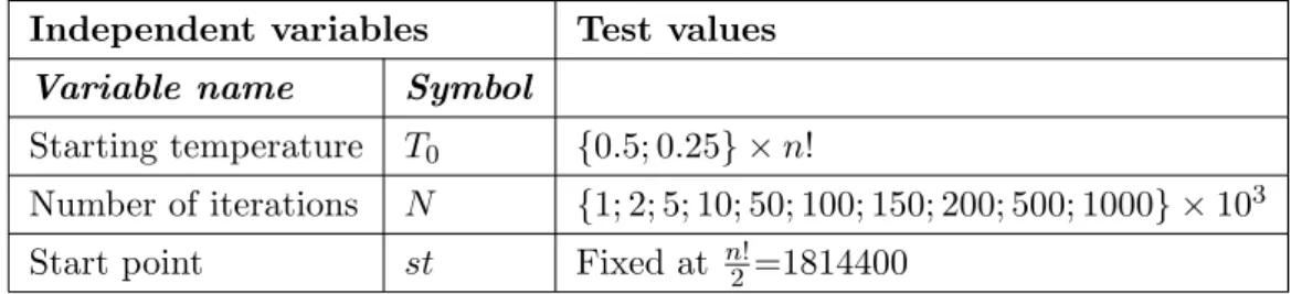
5.1.2 Experimental set-up . . . 67
5.2 Simulated Annealing as the base case. . . 67
5.2.1 Significance of starting temperature on percentage deviation. . . . 69
5.2.2 The effect of iteration count on percentage deviation . . . 70
5.3 SAM . . . 71
5.3.1 Coarse Metropolis-Hastings . . . 71
5.3.1.1 Different runs with the same settings . . . 72
5.3.1.2 Impact of iteration count . . . 75
5.3.1.3 Impact of number of samples . . . 76
5.3.1.4 Impact of number of sections . . . 77
5.3.2 Reduced search Simulated Annealing . . . 77
5.4 Discussion . . . 79
5.4.1 Overview of Results . . . 79
Contents vii
6 Conclusion 90
A Complexity Classes 94
A.0.1 Big-Oh notation . . . 94
A.0.2 P,N P and N P-complete . . . 95
B Problem instances 96 C Results 100 C.1 Simulated Annealing base case . . . 100
C.2 Metropolis-Hastings simulations. . . 105
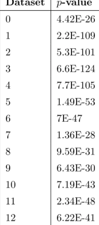
C.2.1 Chi-squared test of significance . . . 105
C.2.2 Impact of iteration count . . . 111
C.3 Reduced search SA final results . . . 112
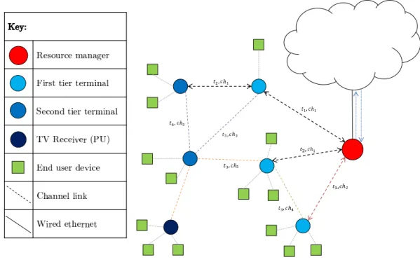
1.1 An example of a wireless network. The resource manager gathers trans-mission requests and allocates each requested flow a specific channel and time slot so as to optimise the overall capacity of the network . . . 5
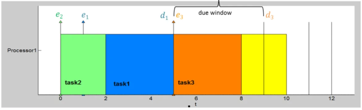
2.1 Example representation of a schedule, showing due window start and end times . . . 10 2.2 A Markov Chain representing states of a Monte Carlo random variable
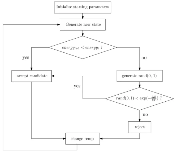
with transition probabilities . . . 17 2.3 Flow chart showing general steps of the Simulated Annealing algorithm. . 26
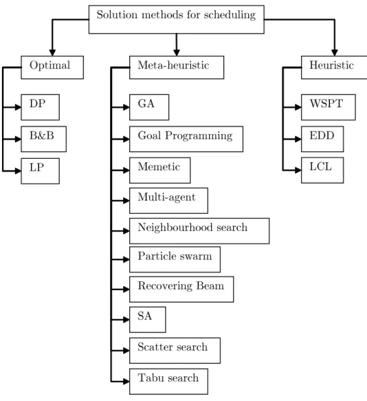
3.1 Taxonomy of solution procedures for scheduling problems . . . 27
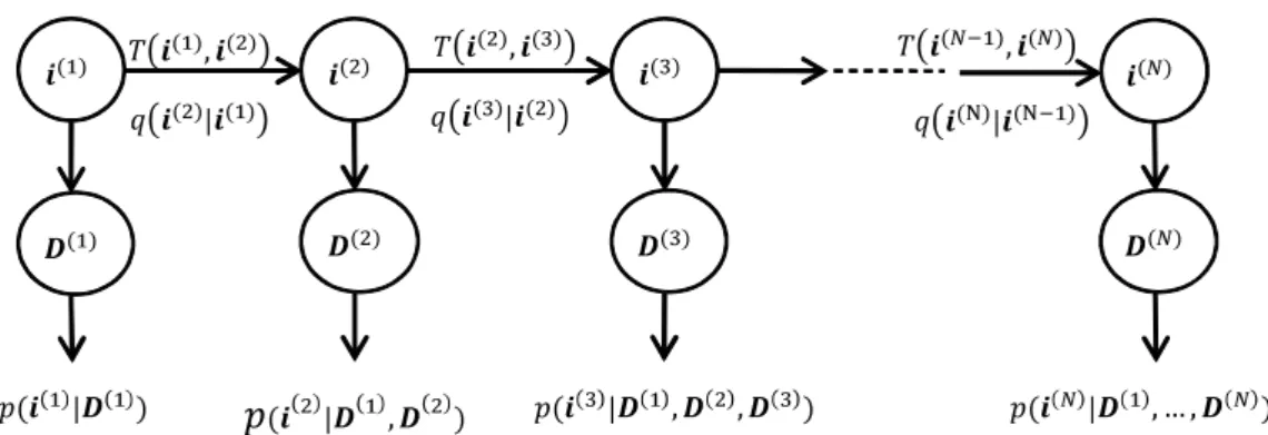
4.1 The evolution of the Markov Chain with sample data gathered on each state change . . . 40 4.2 Bar graph of the indices of the schedule permutations against the inverse
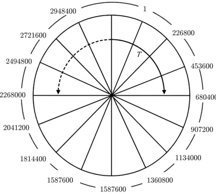
cost of the corresponding schedules. A certain general clustering of similar cost values can be observed . . . 42 4.5 Representation of the set of permutation indices as a wheel with
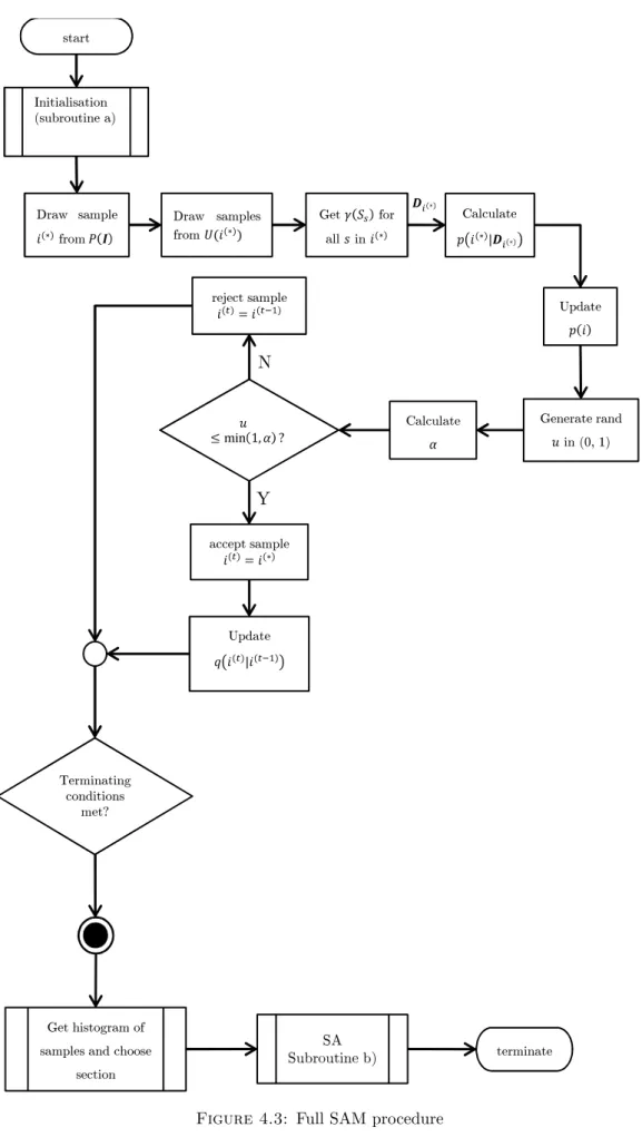
tempera-ture parameter specifying how far around the circumference the algorithm traverses. . . 54 4.3 Full SAM procedure . . . 64 4.4 Initialisation procedure of SAM algorithm.. . . 65
5.1 Normalised frequency distribution by Metropolis-Hastings sampling: prob-lem set with smaller variance . . . 73 5.2 Normalised frequency distribution by Metropolis-Hastings sampling:
prob-lem set with larger variance . . . 73 5.3 Histogram showing the effect of iteration count on the sections selected
by MH: 500 inner samples and 20 sections . . . 83 5.3 Histogram showing the effect of iteration count on the sections selected
by MH: 500 inner samples and 20 sections . . . 84 5.4 Histogram showing the distribution produced by MH with 50, 100, 200
and 500 inner samples, dataset 1. Higher numbers of inner samples result in more concentrated distributions . . . 85 5.5 Histogram showing the distribution produced by MH with 50, 100, 200
and 500 inner samples, dataset 5. Higher numbers of inner samples result in more concentrated distributions . . . 86 5.6 Histogram showing the distribution produced by MH with 50, 100, 200
and 500 inner samples, dataset 10. Higher numbers of inner samples result in more concentrated distributions . . . 87
List of Figures ix
5.7 Histogram showing the distribution produced by MH with 50, 100, 200 and 500 inner samples, dataset 13. Higher numbers of inner samples result in more concentrated distributions . . . 88 5.8 Histogram of the results of SAM, taken over all problem sets, shown
for SAM with 20 MH sections (SAM20), 50 sections and 100 sections (SAM50 and SAM100). The results of basic SA for two different starting temperatures are also shown for ease of comparison. . . 89
C.1 The effect of different run lengths on the frequency distribution for 20 section divisions, 500 inner samples: dataset 1 . . . 111 C.2 The effect of different run lengths on the frequency distribution for 20
section divisions, 500 inner samples: dataset 2 . . . 111 C.3 The effect of different run lengths on the frequency distribution for 20
section divisions, 500 inner samples: dataset 3 . . . 112 C.4 Comparison of percentage deviation of the results from basic SA with two
temperatures, SAM20, SAM50 and SAM100 for run lengths indicated by the iteration counts on the x-axis: dataset 0 . . . 121 C.5 Comparison of percentage deviation of results from basic SA with two
temperatures, SAM20, SAM50 and SAM100 for run lengths indicated by the iteration counts on the x-axis: dataset 1 . . . 122 C.6 Comparison of percentage deviation of the results from basic SA with two
temperatures, SAM20, SAM50 and SAM100 for run lengths indicated by the iteration counts on the x-axis: dataset 2 . . . 122 C.7 Comparison of percentage deviation of the results from basic SA with two
temperatures, SAM20, SAM50 and SAM100 for run lengths indicated by the iteration counts on the x-axis: dataset 3 . . . 123 C.8 Comparison of percentage deviation of results from basic SA with two
temperatures, SAM20, SAM50 and SAM100 for run lengths indicated by the iteration counts on the x-axis: dataset 4 . . . 123 C.9 Comparison of percentage deviation of the results from basic SA with two
temperatures, SAM20, SAM50 and SAM100 for run lengths indicated by the iteration counts on the x-axis: dataset 5 . . . 124 C.10 Comparison of percentage deviation of the results from basic SA with two
temperatures, SAM20, SAM50 and SAM100 for run lengths indicated by the iteration counts on the x-axis: dataset 6 . . . 124 C.11 Comparison of percentage deviation of results from basic SA with two
temperatures, SAM20, SAM50 and SAM100 for run lengths indicated by the iteration counts on x-axis: dataset 7 . . . 125 C.12 Comparison of percentage deviation of the results from basic SA with two
temperatures, SAM20, SAM50 and SAM100 for run lengths indicated by the iteration counts on the x-axis: dataset 8 . . . 125 C.13 Comparison of percentage deviation of results from basic SA with two
temperatures, SAM20, SAM50 and SAM100 for run lengths indicated by the iteration counts on x-axis: dataset 9 . . . 126 C.14 Comparison of percentage deviation of results from basic SA with two
temperatures, SAM20, SAM50 and SAM100 for run lengths indicated by the iteration counts on x-axis: dataset 10 . . . 126
C.15 Comparison of percentage deviation of the results from basic SA with two temperatures, SAM20, SAM50 and SAM100 for run lengths indicated by the iteration counts on the x-axis: dataset 11 . . . 127 C.16 Comparison of percentage deviation of the results from basic SA with two
temperatures, SAM20, SAM50 and SAM100 for run lengths indicated by the iteration counts on the x-axis: dataset 12 . . . 127
List of Tables
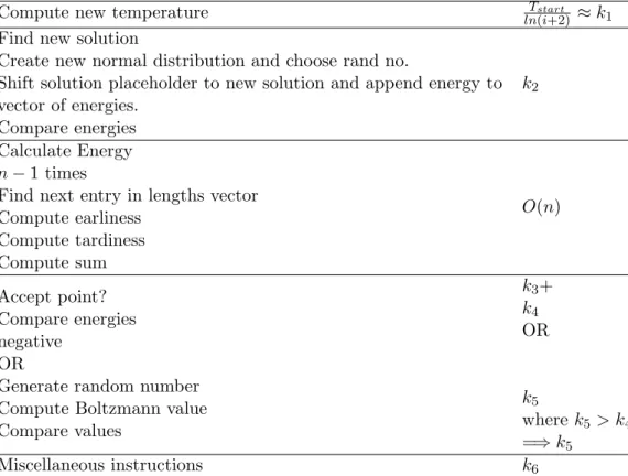
4.1 Calculating computational complexity of components of the SA algorithm 59
5.1 Parameter values used for evaluation of SA Full search . . . 68 5.2 Summary of averages of all results - basic SA . . . 68 5.3 Significance of iteration count by p-values per dataset . . . 70 5.4 0.99 percentiles of maximum percentage deviations for run lengths given
by the iteration count . . . 71 5.5 Unnormalised frequency with which each section (out of 20 sections) was
selected in 20 runs of MH, with thep-values of Chi-squared test: Dataset 0 74 5.6 Average percentage deviation of reduced search SA results compared with
full search basic SA. . . 78
B.1 Problem Instances . . . 96
C.1 Summary of SA results. . . 100 C.2 Dataset 0 MH: Summary for division of search space into 100 sections,
part 1 . . . 106 C.3 Dataset 0 MH: Summary for division of search space into 100 sections,
part 2 . . . 107 C.4 Dataset 0 MH: Summary for division of search space into 50 sections, part 2108 C.5 Dataset 0 MH: Summary for division of search space into 20 sections, part 1109 C.6 Dataset 0 MH: Summary for division of search space into 20 sections, part 2110 C.7 Summary of results of reduced search SA compared with full basic SA . . 113 C.7 Summary of results of reduced search SA compared with full basic SA . . 114 C.7 Summary of results of reduced search SA compared with full basic SA . . 115 C.7 Summary of results of reduced search SA compared with full basic SA . . 116 C.7 Summary of results of reduced search SA compared with full basic SA . . 117 C.7 Summary of results of reduced search SA compared with full basic SA . . 118 C.7 Summary of results of reduced search SA compared with full basic SA . . 119
B&B Branch and Bound CPU CentralProcessing Unit CTS CleartoSend
DP Dynamic Programming EDD Earliest Due Date GA GeneticAlgorithm
IEEE Institute of Electrical and Electronic Engineers LCL Least CostLast
LTE Long TermEvolution
MAC MediumAccessControl (layer) MCMC Markov Chain MonteCarlo MDP Markov Decision Process MH Metropolis-Hastings
NDTM Non-deterministicTuring Machine NP Non-deterministicPolynomial NSE NumericStandard Error p.d.f. probability densityfunction PHY Physical (layer)
QoS Quality of Service RDD Relative Due Date RTS Request to Send SA Simulated Annealing
SAM Simulated Annealing with Metropolis-Hastings sampling SSDP Successive Sublimation Dynamic Programming
SPT Shortest Processing Time
Abbreviations xiii
SRPT Shortest RemainingProcessing Time TS Tabu Search
J set of jobs
j index referring to a single job pj processing time of job j
dj end of due window of job j ej start of due window of job j
sj starting time of job j Cj completion time of job j
w0j earliness weight of job j w00j tardiness weight of job j Ej earliness of jobj
Tj tardiness of job j
≡ identical to
P(X)≡PX probability distribution p(X=x)≡p(x) single probability value
IEPX[f(x)] expectation of the functionf(x) over the probability density function PX
γ ≡ P j∈J
(w0jEj+w00jTj) cost function to minimise
∨ OR
∧ AND
U(a, b) uniform distribution of real numbers between aand b
|S| size of object or set S. IfS is a set this is equal to the number of elements in S
Chapter 1
Introduction
1.1
Background
Scheduling can be described as the allocation of a set of tasks over any sparse resource in order to optimise certain objectives [1]. The applications are as numerous as the field of engineering is broad, making this an important area of research. With a history of research mainly centred on the manufacturing industry, traditional scheduling methods may come short of meeting the needs of more modern applications, where results may be more time-sensitive. In Telecommunications, for instance, tasks such as data packets may be cleverly scheduled in time or frequency domains, or both, in order to maximise data throughput. This needs to be done quickly enough to ensure the user experience is not negatively affected. Being typically an N P-hard or N P-complete problem – even with just one machine or processor, and a single optimisation objective – meta-heuristic algorithms are the accepted solution technique since no optimal polynomial time algorithm exists (unless P = N P) [2]. Finding the optimal solution is as easy as finding the proverbial needle in a haystack – without a magnet or other metal detector.
Some common algorithms used to date are Genetic Algorithms (GAs), Tabu Search (TS) and Simulated Annealing (SA), as well as Particle Swarm optimisation, to name but a few. These may provide acceptable answers in a much shorter time than optimal methods or the brute force approach, but there is still a time cost to pay. If a general way can be found to reduce the solution search space and reduce run times without eliminating potentially “good” solutions, this would be of great benefit to a variety of industries.
A few questions now emerge:
i) What algorithm to choose out of the ocean of possible options?
ii) Can any algorithm categorically be named the best?
iii) Can algorithms be combined to exploit advantages of each?
iv) Can performance be improved by adding pre-sampling to prune the search space?
It is not the aim of this work to answer all these questions but it does aim to shed some light onivand to some extentiii. We have chosen the Simulated Annealing algorithm as the basis, partly motivated by an apparent shortage of research using this algorithm for the sum of weighted earliness and tardiness even though it appears to be an attractive option, but also owing to its comparative computational simplicity and shorter running time over the often-preferred Genetic Algorithm. Further justification of this choice can be found in Section 1.3.3 It is not by any means contended that this algorithm always displays better performance than others, and this is indeed irrelevant to the purpose of this work. Simply, the aim is to investigate the hypothesis that pre-sampling methods can be combined successfully with a basic SA algorithm in an advantageous way. A full motivation is presented in Section1.3.
Although algorithms have become increasingly sophisticated and a number of options exist when a scheduling problem is to be solved, there is still a limit to the size of the problem for which we can find optimal solutions because the inherent computational complexity results in long running times. For scheduling problems this is of particular concern as the number of permutations (and thus the search space) grows very fast with the number of jobs. When fast results are required or the number of tasks is even as modest as ten, a method is required to reduce the time to obtain an answer of acceptable quality, as determined by the particular context. The question arises whether any gain can be had from combining techniques to trade off the strengths and weaknesses of each. SA is a fitting general algorithm to use when little is known of the problem and the search space does not follow any identifiable pattern or trend. The latter may seem true of scheduling problems in general but on closer investigation it may be seen that certain areas of the search space could be eliminated early in the search process to prevent the algorithm wasting time foraying into sections that statistically are unlikely to contain the optimal answer. Pre-sampling may offer a way to prune early without counterbalancing this improvement with more complexity.
In this work it is investigated if the performance of Simulated Annealing can be improved by combining the SA algorithm with other sampling methods in a two-step process. The focus thus turns to efficient sampling methods. Probably the most powerful sampling method available at this time is Markov Chain Monte Carlo (MCMC) methods based on Bayesian inference.
3
1.2
The Problem
The problem is to apply, or devise, and test an algorithm that is able to find solutions to single machine scheduling problems in a relatively short time period that are mini-mally deviant from the optimal value. Since the number of possible scheduling problem instances is infinite, our experiments are confined to a few instances only, which we con-tend are sufficiently representative for the results here to be of more general significance. Performance is evaluated in terms of the running time and quality of the solution: on the basis of analysis of the worst-case complexity, and percentage deviation from the optimum value, respectively. While we note that there are limitations to characterising run time by worst-case complexity analysis, a concern raised by Hall and Posner [3], this method is more fair for the purposes of a comparative study than measuring running times in seconds, since it enables the evaluation to be independent of implementation de-tails and bias that would inevitably arise from the way a programmer writes the code for the different methods, or from platform differences (operating system, processor etc.).
We now list assumptions necessary to narrow the focus of the problem and provide a springboard for solutions.
Assumptions:
• The processing times of jobs are knowna priori to the scheduling activity and all jobs are available at the start of the scheduling activity.
• Machine idle time is not allowed or required and no set-up time is considered.
• No pre-emption is allowed.
• There are no precedence relationships between jobs, so that any sequence of jobs is a feasible solution.
• The problem instances tested are sufficiently representative of real problem sets in as far as proving the methodology to be presented is valid and for relative performance evaluations to be at least indicative of expected results for any given problem instance.
The scheduling goal is to minimise the total weighted amount of time by which each job is completed outside of its due window, and we seek an efficient solution (i.e. one that satisfies the conditions given by eqn. (1.2)). This is anN P-hard problem [1,4,5]. Since machine idle time is considered unproductive and assumed unnecessary, it is not
considered in this work; consequently the scheduling decision involves only the order in which jobs are to be scheduled so as to minimise the scheduling objective, eqn. (1.1)
minγ =minX j∈J
(w0jEj+w00jTj) , (1.1)
where jobs are given unique due windows (not just due dates) and earliness (Ej) and tardiness (Tj) carry different penalties per job, wj0 and wj00, respectively. Please note that clarification and illustration of elements of scheduling are given in Section2.1.
A scheduleSis said to be efficient if there does not exist another scheduleS0 satisfying,
over all j∈J, max j [w 0 jEj(S0)]<max j [w 0 jEj(S)] ∧ max j [w 00 jTj(S0)]<max j [w 00 jTj(S)] . (1.2)
The null (H0) and alternate (Ha) hypotheses investigated are:
• H0: A combination of Simulated Annealing and Metropolis-Hastings Markov Chain
Monte Carlo psampling (to prune the search space) cannot be found that re-duces the running time of SA (on the full search space) for the problem instances presented.
• Ha: A combination of Simulated Annealing and Metropolis-Hastings Markov Chain Monte Carlo pre-sampling (to prune the search space) can be found that reduces the running time of SA (on the full search space) for the problem instances pre-sented.
To this point, we have evaded defining what a “reasonable”, “acceptable” or “good” solution would be, since this is situation dependent and relative. Similarly, ambivalent terms for run times are used. For the problem instances investigated in this work, the issue has been circumvented by comparing results on a relative scale, and categorising solutions depending on their statistical properties. Detail on this is given in Chapter5.
1.3
Motivation
1.3.1 Possible applications
Optimal scheduling of resources is a popular area of research with an almost inex-haustible list of possible application areas. Benefit can be derived by a number of
5
industries from improvements in algorithms for the purpose. Scheduling was first ap-plied in the industrial engineering realm for ensuring Just-in-Time delivery in factories by scheduling when unfinished materials were to be processed on each machine along the production line. Scheduling is very useful in Distributed Computing environments to allocate computing resources to users, or to schedule CPU threads optimally [6]. Scheduling has been used to find optimal task and time allocation strategies for the people working on large software projects, each with different skill levels for different tasks [7], and has also been used for scheduling of maintenance activities on electrical generators [8]. These are just a few examples.
Figure 1.1: An example of a wireless network. The resource manager gathers
trans-mission requests and allocates each requested flow a specific channel and time slot so as to optimise the overall capacity of the network
A very pertinent and topical application of this algorithm is in wireless communication networks where devices have limited access to channel and time slot resources. In recent years the issue of spectrum scarcity has become quite contentious and has sparked a fair amount of research activity into more optimal ways to allocate and use spectrum resources [9–11]. In order for varying Quality of Service (QoS) requirements to be met, different packets to be transported in the network may have different penalties related to their QoS level. Tardiness relates to throughput delay while, in such networks, if a packet is sent too early collisions may occur, thus prompting a series of retries and ultimately causing further throughput delays. Possibly, the destination may still be processing a previous frame and clearing its buffers, causing the frame to be lost and requiring further
transmission retries. Limited buffer size may be a pertinent problem in power low-cost Wireless Sensor Networks. This may be the case in mesh and other networks where non-cooperative coexistence methods are employed. If, instead, the specific channel and time slot allocations to optimise these criteria are decided upon in advance by a channel or resource manager entity, collisions can be avoided and optimal use made of a channel as soon as it becomes available. Such a managed situation is illustrated in Figure 1.1. In the figure, ti represent time slots andchi are wireless channels.
In most current wireless standards (such as IEEE 802.11af, 802.19.1, 802.16-2012, 1900.4), the MAC/PHY includes the architecture and data types to enable a managing entity such as the channel manager of 802.19.1 to allocate resources to devices based on cer-tain objectives and using an on-board algorithm [12–14]. An application may be where nodes must first send RTS control frames containing the size of the data packet to the manager before continuing with the transmission. An example of a network with flows (links) allocated over time and channels (frequency) is illustrated in Figure 1.1. While protocol mechanisms are provided for the interaction mechanisms of the manager and its terminals to broadcast assigned channels, few specific algorithms are provided for the actual scheduling decision to be made. The algorithms presented in this work can be run by the management entity for network channel or time slot allocation, or both, in terms of IEEE 802.19.1, IEEE 802.22 [15] and other standards. The algorithm can be run on the channel manager node while waiting for channel availability and then when it becomes available, spectrum utilisation during the short assigned time slot can be improved. The algorithm may also be suited to wired networks.
1.3.2 Usefulness of more research on scheduling
While a fair body of literature exists in which SA is used to solve the single machine scheduling problem and a little has been done that deals with the specific optimisation criterion of weighted earliness and tardiness, most literature does not show in depth how the performance is influenced by the various parameters or quantify what performance can be expected for different combinations of values of the parameters, nor do they show how the parameters interact and influence one another. There is also no other work that applies and uses Metropolis-Hastings sampling in the unique way we do here or uses pre-sampling or hybridises pre-sampling with SA to produce a more efficient algorithm. This fact emerges from the literature reviewed in Chapter3.
The main contribution of this work is to add a pre-sampling step that enables a significant reduction in the search space before running the SA algorithm on scheduling problems in a way that enables low-cost solutions to be found much more efficiently than by the basic
7
SA algorithm alone. We present a unique application method and implementation of Metropolis-Hastings Monte Carlo to a problem that has not been done in the literature, as far as the author is aware, and that recognises and uses specific properties of the search space in solving this particular problem. We also investigate in detail the influence of parameters on the performance of the basic SA approach and introduce a new neighbour generation method that can be used in many meta-heuristic scheduling algorithms. This neighbour generation method relies on a new way of visualising the search space.
1.3.3 Why Simulated Annealing?
As is illustrated by the summary of previous work on the topic of heuristic algorithms for scheduling (Chapter3), a number of algorithms have been used and have seen varying degrees of success. It has been claimed that the GA is a very, if not the most, successful meta-heuristic. GAs, however, have some disadvantages.
GAs are complex and require a number of further calculations and operations between iterations beyond the basic steps. For example, the mutation operator typically requires a number of operations and calculations to be performed to ensure the offspring created by the crossover operator are feasible [16–18]. These operations are typically complex. Additionally, the mutation operator must be applied either every iteration or when the best value found remains unchanged for a predetermined number of iterations. In the latter case, the operator must be applied as many times as the value remains unchanged, adding further complexity. In some cases a quantity such as the entropy within a gen-eration is calculated first in order to determine the number of times the operator is to be executed [18]. All of these operations and calculations are particularly costly, adding time that is not affordable in today’s highly time-sensitive applications.
In each generation a large number of solutions is considered and every time a new solution is created by the genetic operators, the chromosomes must be placed into their ranking order once again, necessitating a sorting algorithm to be run on the chromosomes of every generation. Even a relatively cheap sorting algorithm of O(nlogn) run 1000 or even 100 times is very costly, particularly for large population sizes, e.g. where n is of the order of 200.
Adewole et al. performed a detailed comparison of SA and GAs as applied to the travelling salesman problem [19]. They conclude that GAs can provide a high quality of solution over SA but under the condition that the population set is large enough. Large population sizes in turn increase the complexity and running time exponentially. The researchers note that if powerful parallel computing capability is available, GAs can perform very well and reach solutions in shorter time periods. Noting our intended
application area of wireless networks, this implies that GAs would be most useful in a fully distributed wireless network where all nodes have powerful computers on-board and can run parallel streams of populations. However, such fully distributed networks, where computing power can be shared, are not yet commonplace and are not the intended application scenarios for our work. Applications where GA meta-heuristics are chosen are typically less time-sensitive and more quality-centric. Examples are component placement in circuit design [20] or flight scheduling [21].
TS has also been used frequently but, as Raaymakers and Hoogeveen remark, requires significant tailoring to the specific problem [22].
In contrast, SA is generally applicable and relatively simple to implement. It requires only sampling a solution, calculating the Boltzmann quantity and comparing the result with a chosen random value. Solution quality provided by SA may not be as high as when using GAs but the running time is significantly lower. We have chosen SA as it is less complex and its implementation is simpler than GA but the method still offers the benefits of being able to escape from local optima and a minimal prior knowledge of the search space, while yielding acceptable solutions. In the intended application area of a centralised wireless network, obtaining a solution in a short space of time is more important than obtaining a solution that is very close to optimal (or is possibly optimal) but causes significant delays. The formulation of the problem as an SA problem is also well suited to the method we introduce to prune the search space.
1.4
Overview of Dissertation
The main contributions of this dissertation are to:
• Introduce a new neighbour generation method that can be used in meta-heuristic single machine scheduling algorithms.
• Introduce a new combination algorithm of Metropolis-Hastings pre-sampling and Simulated Annealing, which we call SAM, for the solution of single machine scheduling problems with due windows and without pre-emption, where idle time is not allowed, and set-up time is not required, and present a comparison of perfor-mance results from and theoretical computational complexity of basic Simulated Annealing, and the proposed hybrid algorithm.
In Chapter2we first go through some preliminary theoretical and foundational concepts, models and definitions to provide a sufficiently complete introduction to the work that
9
follows. Chapter 3 presents some of the more pertinent literature related to this work. The design and details of my specific implementation of SA and a thorough description and development of the new hybrid algorithm of coarse Metropolis-Hastings sampling and SA is presented in Chapter 4. Chapter 5 contains a presentation and analysis of simulation results of the algorithms before we conclude in Chapter 6.
Preliminaries: Models,
Definitions and Techniques
2.1
Scheduling Theory
2.1.1 Notation and Definitions
The essential theory of scheduling that may aid understanding of the work presented in this dissertation is briefly presented here. This is drawn from some well-known literature in the field, in particular the definitive work by Pinedo [5], and is not intended to be any more comprehensive than necessary.
Figure 2.1: Example representation of a schedule, showing due window start and end times
Figure2.1illustrates elements of the general scheduling problem. The general scheduling problem is defined by a set ofnjobsJ = (J1, J2, ..., Jn), which are to be scheduled on a set of m machines or processors M = (M1, M2, ..., Mm). For the purpose of this work, it is assumed that a machine can only process one job at a time. If a machine is able to process a number of jobs simultaneously, this is called batch scheduling. Each job
11
j ∈J can be characterised by its processing time on machine i (pij), its due date (dj) and a possible weight (wj) or set of weights (w0j and wj00) for earliness and tardiness, which indicates relative importance. The job start time is denotedsj. The subscripti denoting the processor is omitted in the single machine case. We generalise the due date into a due window within which a task must be completed to prevent carrying earliness or tardiness penalties. The beginning of the due window is given by ej and the end of the due window by dj as illustrated in Figure 2.1. The weighted earliness of job j is defined aswj0Ej and the weighted tardiness asw00jTj. The job’s actual completion time is Cj. If pre-emption is not allowed, i.e. all jobs must be completed without interruption, we defineCj =sj+pj.
For a job with due window, earliness is defined as eqn. (2.1)
Ej =max{ej−Cj; 0} (2.1) and tardiness as eqn. (2.2)
Tj =max{Cj−dj; 0}=max{Lj; 0} (2.2) The schedule may have to allow for idle time on the machine(s) for maintenance, setting up or during faults or breakdown.
A schedule is feasible if no two jobs are overlapping and no job starts earlier than the schedule start time, i.e the condition of eqn. (2.3) is met.
{si ≥Cj ∀i > j} ∧ {si ≥t0} ∀i, j∈J (2.3)
The scheduling problem is described using the traditional three-field notation,hα|β|γ i [1], where
– α describes the processing environment. For single machine problems, this value is simply 1.
– β describes the constraints. These could include a release date rj when the job initially becomes available for processing, set-up time, precedence constraints, pre-emption or any of a variety of other constraints.
– γ is the objective function. Some examples are the makespan (maximum com-pletion time), total comcom-pletion time (the sum of comcom-pletion times of all jobs) or total weighted completion time. The total earliness and tardiness of jobs, either
separately or jointly ( defined in eqn. (2.4) ), are also common functions to be minimised (and the objective function of this work).
γ =X j∈J
(w0jEj+w00jTj) (2.4)
Numerous models of the scheduling problem exist, each having very different meth-ods that may provide the best results. Some variants to the model include situations where set-up time is considered as a cost separately from the processing time, where pre-emption may or may not be allowed, and where processing is either batched or non-batched. Schedule models with several processors include parallel-machine, where machines may be identical or differing in capabilities and/or speeds; flow-shop, where each job has to go through a series of different processors before being complete; and flex-ible flow-shop, a generalisation of flow-shop; job-shop, which is still further abstracted in that each job may have an independent set of processes to follow, and open-shop processing, where jobs are to be processed on each machine in any order. Models may define deterministic job characteristics or may be stochastic, such as in the Markov Deci-sion Process approach [23]. A newer model that has emerged is multi-agent scheduling, where each agent is responsible for a certain set of jobs and has its individual set of objectives to optimise.
With so many more complex models in existence, it may be necessary to justify the practical applicability of the model we have chosen for our analysis. A large number of practical problems are in fact accurately reflected in the single machine model [5,24–26]. Examples may include a number of tasks or task segments to be processed by a single CPU. Even if there is more than one CPU in such a situation, the units often func-tion independently in parallel and thus are decomposed into separate single processor problems and solved independently. The decomposition of multi-machine problems into single machine problems is often done [5] and so this model provides a good fundamental basis for analysis, and results can easily be extended to apply to more complex prob-lems. The situation where pre-emption is not allowed has been chosen as this is also a generalised form of the problem, and the model can easily be adapted to situations with pre-emption allowed. For example, jobs can be divided into arbitrarily small pieces and scheduled as separate tasks to model situations where pre-emption is allowed. The crite-ria of weighted earliness and weighted tardiness are very common measures in industcrite-rial settings and several other just-in-time applications, and are recognised in the literature as important for research focus [4,16,27–31]. The problem as it stands is already known to be strongly N P-hard [4,26,32–34]. In fact, even the problem considering only one objective h1||P
j∈Jw00jTji is known to be a strongly N P-hard problem [5]. Thus, our problem is complex and practically applicable enough to justify investigation, and to
13
justify investigation into evaluating and improving the performance of meta-heuristic algorithms to solve this type of problem.
2.1.2 Priority dispatch rules
Some theorems on the prioritisation of tasks, known in the literature, are briefly pre-sented here. These may be optimal for certain simpler single-criterion scheduling prob-lems but are not optimal for the problem of this work. We present them as they form a starting point for a number of solutions presented in the literature.
Theorem 2.1 (Shortest Processing Time (SPT) [5]). When minimising completion time, an optimal schedule is found by sorting jobs in increasing order of processing time.
This is called the Shortest Processing Time (SPT) and Shortest Remaining Processing Time (SRPT) rule, which also extends toWeighted Shortest Processing Time (WSPT).
Proof. The reason emerges from the equation for total completion time shown below for the unweighted case ( eqn. (2.5) ) and weighted case ( eqn. (2.6) ). These equations show that when schedulingN jobs, the first job’s processing time is addedN times,p2 is
addedN−1 times,p3 addedN−2 times and so on, so to minimise the total completion
time it is necessary to start with the shortest, and end with the longest processing time.
X j Cj = (t+p1) + (t+p1+p2) + (t+p1+p2+p3) +... (2.5) X j Cj = (t+p1)w1+ (t+p1+p2)w2+ (t+p1+p2+p3)w3+. . . (2.6)
Corollary 2.2. The WSPT heuristic processes the values pj
wj in non-decreasing order,
where wj is the weighting given to job j, as shown by eqn. (2.7):
p1 w1 ≤ p2 w2 ≤ ...≤ pn wn . (2.7)
Building on from these rules, certain problems may enable the assumption of restrictions on processing times and weights. These theorems are presented and proved by Yano and Kim [27]. These are:
Theorem 2.3. For adjacent jobs i and j with starting time si ≥ sj, it is optimal to
sequencei before j if and only if the conditions given by eqn.(2.8) to (2.11) are met.
Ei/Ej ≤pi/pj (2.8) and pi/pj ≤Ti/Tj (2.9) and Eipi+Tjpi ≤(Tj+Ej)(sj −si+pj) (2.10) or Ei+Ti ≤Tj+Ej (2.11)
Proof. The proof is presented in [27].
Theorem 2.4 (Earliest Due Date (EDD) [35]). Jobs are to be sorted into increasing order of due dates to obtain an optimal schedule for minimising maximum lateness or maximum tardiness.
Proof. Full proof in [35]. Intuitively, jobs with earlier due dates are in greater danger of being later than their due date than jobs with later due dates, so to obtain an optimal schedule, these must be scheduled first. Where jobs are weighted, the weighted due date must be used.
Theorem 2.5 (Least Cost Last (LCL) [36]). Jobs with the lowest weighted cost are scheduled towards the end to solve the general h1|prec|fmaxi in O(n2) time.
Proof. Full proof in [36]. As the rule is an extension of EDD, similar to the EDD rule, this aims to minimise the total cost of the schedule.
The techniques above, and extensions to these, are heuristic techniques rather than algorithms and are specific to scheduling problems. They are called “constructive” since they gradually build up a schedule using certain rules [5].
2.2
Algorithms
Meta-heuristic algorithms find either approximate solutions to optimisation problems, or solutions to not all instances [37]. Most do this by starting with an initial solution and then searching the space of all possible solutions to improve on it. Meta-heuristic
15
algorithms such as Genetic Algorithms, Simulated Annealing and Tabu Search have been used to solve scheduling problems but can be applied to any of a wide variety of other optimisation problems. Deterministic or exact algorithms in contrast can be used to find the optimal solution but their time complexity for large problems may be unacceptably high in cases. Two of these optimal methods are dynamic programming and the branch-and-bound algorithm. Branch-and-Bound is often cut short to reduce computation resulting in only a suboptimal solution, when the gap between the upper and lower bounds becomes acceptably small. Complexity is a key consideration in the choice of algorithm. We formalise the notion of complexity classes and appropriate definitions in AppendixA.
2.3
A Note on Notation
Some points about the notation used are necessary to avoid ambiguity. I have tried to be as consistent as possible in this respect. Random Variables (R.V.s) are given as capital letters (e.g. Y and X) unless otherwise stated. Sample spaces are given by similar notation. The terms observation, random draw and sample are equivalent.
i) A single observation of a scalar R.V. is denoted e.g. x, y or, explicitly, X=x.
ii) A set ofnrandom draws from a scalar R.V. is denoted as x={x(1), x(2), ..., x(n)}. iii) A row vector of sizeD is writteny= (y1, y2, ..., yD).
iv) Thenth sample of the vector R.V.Y=y, is y(n)= (y1, y2, ..., yD)(n).
v) A set of n random draws from a multidimensional or vector R.V. is in bold print e.g. x={x(1),x(2), ...x(n)}.
vi) The probability density function (p.d.f.) of a random variable over the set of all possible values is written in uppercase P(X) orPX, while the probability that the random variable takes on a specific value is written in lowercase p(X=x).
vii) A set of values that occupyd-dimensional space may be denoted Sd⊂IRd.
viii) The term “distribution” is used in this context to mean p.d.f. P and the terms are used interchangeably. This is in keeping with the usual literature on the topic, though it is noted that “distribution” may also refer to the cumulative distribution function in other texts.
ix) Conditional expectations will use the notation:
IEπ(x|y)[f(x)]
for example, which is equivalent to
IEx[f(x)|y] = Z
x
p(x|y)f(x)dx .
x) One final note applicable in particular to the results (Chapter 5), where we make a perhaps sacrilegious return to frequentist techniques for evaluation and results analysis, is that a p-value of 0.05 or less for statistical significance tests such as Chi-squared and t-test, is considered statistically significant.
2.4
Bayesian Inference
Bayesian probability is an integral part of all Machine Learning algorithms, since it provides a method by which inference about the future can be made from previous observed data or about latent variables, given observed data variables [38]. Bayesian probability exploits dependencies between data samples, rather than assuming or forc-ing an artificial independence. The application of Bayesian statistics to MCMC has been directly responsible for the great popularity that MCMC has seen in recent times, enabling characterisation of complicated posterior distributions such as parameters in complicated system models [39].
Scalar R.V.s are used to illustrate concepts for clarity and to avoid the messy notation of Jacobians that would be required otherwise. Bayes’ theorem states that, given sample data y ∈S1 ⊆ IR from a distribution with known likelihood P(y|x), a posterior
distri-bution π(x|y) (given by eqn. (2.12)) for unknown variable x∈S2 ⊆IR can be inferred
from an a priori density for x given by P(x) via the conditional probability, as shown in eqns. (2.12) and (2.13):
π(x|y) ∝ P(y|x)P(x) (2.12)
where the constant of proportionality is
Z
x∈S2
17
The expression P(x) captures initial assumptions aboutx before the observation. The equivalent for discrete random variables, given by eqn. (2.14), is equally valid.
π(x|y) = (P(y|x)P(x)) P(y) = P(y|x)P(x) P S2(p(y|x)p(x)) = PP(y|x)P(x) S2(p(y, x)) (2.14)
wherep(y, x) represents the joint probability ofxand y. We may want to find expecta-tions, such as eqn. (2.15), of a function f(x) over the probability densityπ(x|y):
IEπ(x|y)[f(x)] =
Z
S2
f(x)π(x|y)dx , (2.15) or the discrete equivalent. Clearly, we require that f(x) is integrable with respect to π(x|y). For many problems it may not be feasible to evaluate the integral directly, either because no closed form integral exists or owing to high dimensionality making computa-tion practically prohibitive. In such situacomputa-tions, it is necessary to employ approximacomputa-tions or relaxation techniques. Such problems are very common and this is where Monte Carlo techniques shine.
2.5
Markov Chains
xଵ x xଶ xଷ x
ሺଵሻxሺଶሻ xሺଶሻxሺଷሻ xሺିଵሻxሺሻ
Figure 2.2: A Markov Chain representing states of a Monte Carlo random variable
with transition probabilities
A Markov Chain, such as illustrated in Figure2.2, is a series of states or random variables with memory representing a stochastic process so that the value or probability of a state depends on previous state(s) and the dependency relationships can be represented by transition probabilities, Tm. If a state depends only on its immediate predecessor, the Markov Chain is said to be first order; if it depends on its immediate predecessor as well as the one before, the chain is second order and so forth. More formally, for a first order Markov Chain x(1), x(2), ..., x(M), the condition of eqn. (2.16) holds.
P(x(m+1)|x(1), ..., x(m)) =P(x(m+1)|x(m))
≡Tm(x(m), x(m+1))
∀m∈ {1, ..., M −1} ⊆IN
For the purpose of MCMC simulation, we require that the chain isergodic, that is, it is required that the distribution P(x(m)) converges (asymptotically) to a single invariant distribution (the equilibrium distribution) whenm→ ∞, regardless of the chain’s start point. Provided that the conditions on the transition probability are met, the invariant or stationary distribution satisfies eqn. (2.17).
P(x) =X x0
T(x0, x)p(x0) (2.17)
2.6
Monte Carlo Simulation
2.6.1 Ordinary Monte Carlo
A number of good texts exist on this topic, which the reader may consult if necessary. We have drawn from Christopher Bishop’s comprehensive text here [38], as well as [39–42], and others cited as needed.
Ordinary Monte Carlo aims to estimate properties, such as expectations, of a certain p.d.f. p(x) by drawingN independent identically distributed (i.i.d.) samples from the distribution of random variables and approximating the density function using a point mass approximation for the density [43], as shown in eqn. (2.18).
P(x)≈PN(x) = 1 N N X i=1 δx(i)(x) (2.18)
Then, expectations are calculated using the usual averaging calculation,
IEN[f] = 1 N N X i=1 f(x(i)) , (2.19)
which tends to the required expectation
IE[f] =
Z
f(x)p(x)dx (2.20)
in the limit lim
N→∞IEN[f]. Now if
19
holds, and noting that for ordinary Monte Carlo samples are i.i.d., we can use Central Limit Theorem to find a normal p.d.f. of the approximation’s error
IEPN[f(x)]−IEP[f(x)] . (2.21) The problem, however, is that all too often it is not feasible to get i.i.d. samples from the required distribution and expectations are intractable or impossible to calculate. That is where Markov Chain Monte Carlo comes to the rescue.
2.6.2 Markov Chain Monte Carlo
The essence of MCMC is that statistical inferences can be made about a system without having to know, or be able to simulate, the exact behaviour of a system or know the form of a function describing the behaviour, and this can be achieved with dependent samples instead of i.i.d. samples. We only need to construct a Markov Chain that has the same equilibrium distribution as the true system in question and employ some Bayesian statistics. The complicated distribution and the constructed distribution are typically related by a constant that is difficult to calculate or for which there is insufficient data to calculate, such as may arise in finding a normalised Bayesian posterior. MCMC nonetheless enables one to gather statistical information about the true system, such as expectations of functions under the distribution. This powerful technique performs well even in the case of high dimensionality.
Suppose we wish to sample from a complicated, unknown or unknowable unnormalised distributionπ(x). We are able to evaluateπ(x) for any givenxup to a certain constant, Xp. This constant would normally involve a complicated integral from the Bayesian inference step and is not known. So we have
π(x) = P(x) Xp
.
We cannot sample fromπ(x) directly so we construct a Markov chain onx∈S⊂IR with incremental transition probabilities T(x, dy), where both x andy ∈S. Marginalisingx, the resultant distribution becomes
Z x∈S p(dx)T(x, dy)dx= Z x∈S p(dx)q(dy|x)dx=P(dy) , (2.22) which is the Bayesian normalising constant. We can now sample from a simpler proposal distribution, the transition probabilityQ(x(i+1)|x(i)). Each time a sample is drawn from
the proposal distribution it is recorded for comparison with the next sample. The distribution as well as the next state drawn thus depends on the current state. This is the Markov Chain. As the number of samples becomes very large, P(dy) approaches π(x). The choice of proposal distribution is arbitrary but its choice influences how fast the chain converges to the desired stationary distribution while the specific update mechanism determines whether a candidate state is accepted or not. In choosingQthere are several subtleties. Details about the conditions to ensure the chain converges to the equilibrium distribution are discussed in Section 2.6.2.3. It is sufficient to say for now that it is usually possible to construct a Markov Chain with the required properties.
Several sampling methods are harboured under the umbrella of MCMC. These include rejection sampling, importance sampling, slice sampling and Gibbs sampling. The focus of our work is on the Metropolis-Hastings method discussed below. One of the reasons for this choice is that it allows for an asymmetrical proposal distribution. Another widely used method, Gibbs sampling, is generally applied to a different problem type where the variables represent parameters of a statistical model to be estimated. The parameters must be able to be partitioned into independent sets and should follow a standard conditional probability density function. In this method all proposed updates are accepted. Not only is our situation not one of parameter estimation and so not well-suited to Gibbs sampling, but the acceptance of all updates increases the required memory to store all states, and the running time. Gibbs sampling is simply a special case of the Metropolis-Hastings algorithm, as is rejection sampling [44]. We prefer the more general method.
Importance sampling is another option, but this is a method only for estimating the expectation of a function and does not generate samples from the distribution [45]. We would like samples to be generated for use in the SA step. Another disadvantage of importance sampling is that there may be a very large error in the estimate since the empirically found variance does not necessarily represent the actual variance to any degree of accuracy. Slice sampling may have been an advantageous option, but Metropolis-Hastings is clearer and simpler to implement.
2.6.2.1 Metropolis-Hastings
The Metropolis-Hastings method provides a way of updating samples in the random walk of a Markov Chain Monte Carlo simulation. We start by specifying three distributions, using the variablez here:
i) Target distribution is the approximation to the desired distribution which we may know up to the normalising constant. This is ˜P(z).
21
ii) Proposal distribution. This is an arbitrarily chosen starting transition probability q(z0|z) used to draw new samples. The aim is to construct the chain so that the samples drawn look like samples from the actual distribution, ˜P(z).
iii) A function that samples from the proposal density.
Now, supposing the first state is z(τ), a candidate point z(∗) is generated from the proposal distribution. The candidate is accepted as the new state with probability given
α(z(∗), z(τ)) =min 1,p(z
(τ))q(z(τ)|z(∗))
p(z(∗))q(z(∗)|z(τ))
!
. (2.23)
In practice, the choice is achieved by comparing the value of α(z(∗), z(τ)) with a value drawn from the uniform distribution in the interval (0, 1) and accepting ifα(z(∗), z(τ)) is greater than this sample. If the candidate is not accepted,z(τ+1) =z(τ). We then draw another sample from the proposal distribution and repeat until the specified terminating conditions are reached. Theoretically, as τ → ∞, P(z(τ)) converges to the desired distribution. Convergence is discussed further in Section 2.6.2.3.
First, a note on the choice of proposal distribution: The success or failure of the MCMC simulation hinges quite heavily on the choice of proposal distribution. If it is too narrow, a large proportion of candidate samples will be rejected and a large number of iterations may be required before any useful information is gained from the sample. In contrast, if it is too wide, a large proportion of samples are accepted and correlations may be high, once again limiting the information conveyed by the samples. The choice of proposal distribution may be the most important decision for an implementer to make, and is the one for which no guidance truly exists.
The existence of a stationary distribution is a sufficient condition for irreducibility. This condition informs the choice of proposal distribution, since the proposal must have a wide enough girth to support the probability of reaching any state in the state space with a positive probability inπ. Both the blessing and the curse is that this guidance on choosing a proposal distribution is not much guidance at all since almost any arbitrary distribution chosen will fulfil the requirement. On the other hand, most distributions may take an insupportably long time before the chain starts to converge.
MCMC is a supremely powerful technique allowing the characterisation of complex sys-tems but one runs the risk of wasting resources with a too-lengthy run or never reaching the equilibrium state. We wish to exploit the power of the system while limiting expo-sure to, or consequence of, this weakness. Our question is whether it is useful to use the technique to pre-sample and get a general idea of the terrain of the problem’s search
space to inform a more focused search, and if this can be done in a way that saves rather than compounds overall complexity when in combination with a local search heuristic. Such questions are addressed in Chapters 4 and 5, but are greatly influenced by the implementation issues we now put forward.
2.6.2.2 Burn-in
A common practice in MCMC is to include a “burn-in” or “thermalisation”, a set of samples drawn and discarded before samples are recorded for use in obtaining the re-quired distribution. The reason for this is usually asserted to be removing biases caused by high initial correlation between samples. Geyer asserts, however, that what is impor-tant is rather to find a good starting point for the chain [41]. He asserts that if we could start the chain somewhere in the middle of the equilibrium distribution, there would be no bias to eliminate, and since there are other methods that can be used to find starting points, there is no theoretically defensible reason for the practice [41]. Unfortunately, if there truly is no knowledge of the posterior distribution there is no way to ensure the starting point fulfils this requirement (or hope). Yet burn-in is still an accepted, most common and expected addition to the Metropolis-Hastings initialisation process.
2.6.2.3 Convergence
To ensure that the chain does in fact converge, it is required that the system has the property that starting from any point (vertex if we consider the chain a graph) in the state space, an infinite random walk will always end at a certain point v. Since the Markov Chain constructed is ergodic and stationary with respect toπ(x), ifX(t)∼π(x), necessarily X(t+1) ∼ π(x) for all t, so X is converging to π. The condition of general balance (eqn. (2.24)) must hold for a stationary distribution π, i.e.
πT =π , (2.24)
whereT is the transition probability matrix, which leaves the distribution unchanged.
Restrictions on the transition probability to ensure convergence (and ergodicity) are:
• Connectedness, which implies irreducibility- there is a positive probability of transitioning from any state to any other state. The method requires connectedness so that the same result can be obtained regardless of where the chain starts.
• Aperiodicity- intuitively a periodic function implies that the chain does not end while we require a finite chain.
23
When using Metropolis-Hastings method, one constructs a number of transition prob-ability matrices along the chain, each individually maintaining π but not usually indi-vidually irreducible with respect to the state spaceS [39]. In the case of a chain of such transition probability matrices, we require eqn. (2.25):
X
x∈S
π(x)T(x, x0) =π(x0) (2.25)
to hold forx, x0 ∈S. This condition is both necessary and sufficient to prove invariance. However, since the sum may be intractable to solve, the more stringent condition of detailed balance may be introduced as a sufficient condition. If detailed balance holds,
π(x)T(x, x0) =π(x0)T(x0x) . (2.26)
If each T1, ..., Tn individually maintains detailed balance, so does T. Detailed balance also implies that the chain is time reversible and that Metropolis-Hastings then reduces to a Metropolis sampling.
The difficulty with MCMC methods is that the resultant distribution can only be claimed conclusively to have converged to the equilibrium distribution after infinity iterations. This means there are no better than approximate ways to calculate when to stop the chain of the simulation, and there is no way to know how close an approximation the result is to the real desired distribution.
A number of heuristic techniques are thus required to inform the decision of where to stop the chain. There are a number of different methods which can be compared in order to determine a suitable point of termination. Some are presented below.
Gelman and Rubin
Gelman and Rubin’s method requires that a number of independent parallel chains are run, all with different starting points [46,47]. A factor is then calculated that quantifies how a parameter might shrink if sampling were to be continued indefinitely. The factor includes a comparison between variance of the means of the m parallel chains (B), and them averages of the variances within them chains (W). If the scale factor is close to one, they posit that this means the chains are effectively unbiased by the starting points and likely to approximate the target density. The method involves two steps:
i) Before sampling, it is required that an “over-dispersed” estimate of the target den-sity is obtained so that suitably spread out starting points for parallel chains may be generated.
ii) For each quantity, the lastniterations are used to estimate the target distribution of the quantity using a Student-t distribution.
Using the symbols above, for m parallel chains, where df represents the degrees of freedom, the factor is calculated as
√ R= s (n−1 n + m+ 1 mn B W) df df−2 . (2.27)
While Gelman and Rubin’s method has seen reasonable popularity, there are a few points worth questioning. Firstly, it is computationally very inefficient to run a number of independent chains when the same computation time may have been used simply to run a single chain for longer and possibly get a closer approximation to the target distri-bution. Secondly, the first step of getting over-dispersed samples from the target implies that there must be knowledge of the limits of the sample space, which is unlikely if the point of the MCMC simulation is to infer properties of a distribution without any direct knowledge about it. Thirdly, it involves running the simulation for a certain number of iterations, and then using the lastn to calculate the diagnostic factor. The choice ofn encounters the same problem with which the original Monte Carlo method is afflicted. It may be necessary to repeat this step several times and compare how the factors shrink, costing extra time and computation, which may have been used with equal gain to run the Markov Chain for longer.
Raftery and Lewis
The Raftery and Lewis method assists in determining the length that the Markov Chain in MCMC algorithms should reach, determined by the properties of a short initial “pilot” run [46,47]. The premise is that the ergodic average of the chain is asymptotically normal for large number of samples [44] by the central limit theorem. They estimate the value of nthat ensures thatP(θ−≤θn≤θ+) = 1−α for deviation >0 and 0< α <1 by using the formula,
n≈z}|{ var(θ) Φ−1(1 −α2) 2 , (2.28)
where Φ(·) here denotes the normal cumulative distribution function andz}|{
var(θ) is an estimate of the variance of the ergodic average, based on the observations gained from the pilot run.
Geweke
25
mean of a functiong(θ), this method assumes that the function ghas a spectral density that is continuous at a frequency 0 [46]. A set of MCMC samples afterN iterations can be viewed as a time series. Owing to the properties of Markov processes, the Geweke method considers this a Wide Sense Stationary signal and uses the relationship between the variance of a time series and its power spectral density Sg(ω) (where ω is angular frequency). After N iterations, the estimated expectation of a functiong with respect toθ, is given by ¯ gN = 1 N N X i=1 g(θ(i)) . (2.29)
The asymptotic variance of the series is then given by Sg(0)/N, the power spectral density overN. This estimated standard deviation calculated from the variance is called the Numeric Standard Error (NSE). This value can be calculated at several points until the desired precision is achieved.
The convergence diagnostic functions by taking the difference between means calculated onNAiterations from the beginning of the chain, ¯g(θ)AN, and ¯g(θ)BN, NB iterations from the end, and computing
¯
g(θ)AN −¯g(θ)BN
N SE (2.30)
Geweke suggestsNA to be 1/10 of the total iteration count andNB to be half. Various implementations of the Geweke diagnostic exist, one being to calculate correlations be-tween the two subsets of the total number of samples and determining whether they are sufficiently different.
2.7
Simulated Annealing: The technique
SA is a probabilistic search heuristic used in optimisation problems with complex search space characteristics, such as multiple local optima, first introduced by Kirkpatrick, Gelett and Vecchi [48]. The algorithm models a search on the physical process of an-nealing where a substance is slowly cooled so that freezing occurs at the minimum energy configuration (the, or a, minimum). General requirements are a finite search space, a real-valued cost function, a set of neighbours for each state or neighbour gen-eration method and a non-increasing temperature cooling function. Starting from the first state, the algorithm creates a discrete Markov Chain with the evolution of states in the chain determined on the basis of
Initialise starting parameters
Generate new state
energyt+1< energyt? generate rand(0, 1) accept candidate rand(0,1)<exp(−∆E kT) ? change temp no yes reject no yes
Figure 2.3: Flow chart showing general steps of the Simulated Annealing algorithm.
ii) if the cost of the new state is not lower than the previous value, the state value may still be accepted using a Boltzmann probability distribution. This feature enables the algorithm to escape from local optima.
The general SA algorithm is given in Figure 2.3. The block rand(0, 1) represents the generation of a random real number from a uniform distribution in the range 0 to 1 (excluded). While the SA algorithm is generic, some important aspects of the imple-mentation are mentioned here. Detail about the generation of pseudo-random numbers is important as unintentional biases that may be introduced within the generation method may have unfavourable consequences. The perturbation function for generating neigh-bour states, to be determined by the implementer, depends on the application and is instrumental in the performance of the algorithm.
That concludes all the main background theory and applicable technical information that forms the basis for all the work that follows.