Coordinated Local Metric Learning
Shreyas Saxena, Jakob Verbeek
To cite this version:
Shreyas Saxena, Jakob Verbeek. Coordinated Local Metric Learning. ICCV ChaLearn Looking
at People workshop, Dec 2015, Santiago, Chile. Proceedings IEEE International Conference on
Computer Vision Workshops.
<
hal-01215272
>
HAL Id: hal-01215272
https://hal.inria.fr/hal-01215272
Submitted on 13 Oct 2015
HAL
is a multi-disciplinary open access
archive for the deposit and dissemination of
sci-entific research documents, whether they are
pub-lished or not.
The documents may come from
teaching and research institutions in France or
abroad, or from public or private research centers.
L’archive ouverte pluridisciplinaire
HAL, est
destin´
ee au d´
epˆ
ot et `
a la diffusion de documents
scientifiques de niveau recherche, publi´
es ou non,
´
emanant des ´
etablissements d’enseignement et de
recherche fran¸cais ou ´
etrangers, des laboratoires
publics ou priv´
es.
Coordinated Local Metric Learning
Shreyas Saxena
Jakob Verbeek
Inria
∗Abstract
Mahalanobis metric learning amounts to learning a lin-ear data projection, after which the`2metric is used to
com-pute distances. To allow more flexible metrics, not restricted to linear projections, local metric learning techniques have been developed. Most of these methods partition the data space using clustering, and for each cluster a separate met-ric is learned. Using local metmet-rics, however, it is not clear how to measure distances between data points assigned to different clusters. In this paper we propose to embed the lo-cal metrics in a global low-dimensional representation, in which the`2metric can be used. With each cluster we
asso-ciate a linear mapping that projects the data to the global representation. This global representation directly allows computing distances between points regardless to which lo-cal cluster they belong. Moreover, it also enables data visu-alization in a single view, and the use of`2-based efficient
retrieval methods. Experiments on the Labeled Faces in the Wild dataset show that our approach improves over previ-ous global and local metric learning approaches.
1. Introduction
Metric learning is a machine learning technique with a wide range of applications in computer vision, e.g. lo-cal descriptor matching [10], fine-grained object compar-ison [27], and face verification [22]. Most work con-siders supervised learning of Mahalanobis metrics, see e.g. [9,14,15,22,25,41]. The supervision comes as pos-itive and negative pairs that should be close and far apart respectively. The Mahalanobis distance between two points is given by (xi −xj)>M(xi −xj), where M is a
posi-tive definite matrix. Since M can always be factored as
M = L>L, Mahalanobis metrics are equivalent to the `2
metric after linear projection of the data. For complex class distributions, however, linear projection of the data might not be sufficient to obtain a suitable data representation.
To overcome this restriction, several routes have been ∗LEAR team, Inria Grenoble Rhˆone-Alpes, Laboratoire Jean
Kuntz-mann, CNRS, Univ. Grenoble Alpes, France
explored. First, the linear projection in the Mahalanobis metric can be written in terms of kernel evaluations, see e.g. [14,16,25]. Alternatively, (convolutional) neural net-works with a siamese architecture can be learned to give (dis)similar outputs for positive and negative pairs, seee.g. [5,8]. Approaches based on decision trees have also been explored, seee.g. [27]. Finally, local metric learning uses a collection of Mahalanobis metrics, each operating in a dif-ferent part of the input space, seee.g. [3,4,12,18,20,26,
34,39,41,43]. The partitioning of the space is typically obtained using k-means or Gaussian mixture clustering.
In most existing local metric learning approaches, how-ever, it is unclear how to compute distances between points assigned to different clusters, or distances are defined in an asymmetric manner. Unlike for global metric learning, they can not be interpreted as computing the`2 distance after a
transformation of the data, which hinders data visualization and efficient`2-based retrieval techniques, such as product
quantization and multiple-assignment retrieval [21]. In this paper we propose a solution by embedding the local metrics in a global representation. We use a Gaus-sian mixture model (GMM) to obtain a soft-partitioning of the data. With this partitioning we define a non-linear em-bedding of the input data vectors in a higher dimensional feature space. By learning a Mahalanobis metric over this embedding, we simultaneously learn local metrics for each cluster, and also obtain an alignment of the local metrics. This allows us (i) to compute distances between points re-gardless to which local cluster they belong, (ii) visualize data in a single view, and (iii) use efficient`2-based retrieval
methods. We refer to our approach as “coordinated local metric learning” (CLML).
We validate our approach in face verification and re-trieval settings using the Labeled Faces in the Wild (LFW) [19] dataset, and using image representations based on local binary patterns (LBP) [28], convolutional neural networks (CNN) [42], and Fisher vectors (FV) [35]. For all tested representations our approach improves over global metric learning and other local metric learning approaches. For retrieval, the improvements over previous local metric learning approaches [3,34] are particularly large.
2. Related work
In this section we give an overview of related work that is most relevant to the material we present in this paper.
Mahalanobis metric learning.Many supervised Maha-lanobis metric learning methods exist. Most are based on loss functions defined over pairs or triplets of data points, seee.g. [9,14,15,22,25,40,41]. We refer the reader to recent survey papers [2,23] for a detailed review of these.
Methods based on pairwise loss terms learn a metric so that positive pairs (e.g. points having the same class label) have a distance that is smaller than negative pairs (e.g. points with different class labels). An example of such methods is the logistic discriminant metric learning (LDML) method of Guillaumin et al. [15]. Their obser-vation is that since Mahalanobis distances are linear in the entries ofM, they can therefore be learned via standard lo-gistic regression. In [16] they regularize by instead learning a low-rank factorization that projects the original data to a low dimensional space in which the`2metric is used.
An example of a triplet-based approach is the large-margin nearest neighbor (LMNN) method [41]. Instead of forcing all points of the same class to be close, LMNN re-quires that the nearest neighbors of each point are of the same class. The metric is learned by minimizing a sum of loss terms over triplets of points, where each loss term en-courages the distance betweenxiand neighbors in the same
class to be at least one distance unit smaller than the dis-tance ofxito neighbors in different classes.
Local metric learning. To alleviate the limitations of Mahalanobis metric learning, many local metric learning methods have been proposed, seee.g. [3,4,12,18,20,26,
34,39,41,43]. Here we limit our discussion to five recent state-of-the-art methods.
The R2LML method of Huanget al. [20] jointly learns a set of local metrics and weights,gs
i, that assign data points
xito the local metrics indexed bys. The distance between
xiandxj is computed using the weighted sum of metrics,
where metricsis weighted by the productgs
igsj. They
itera-tively learn the weights and the metrics, updating one while keeping the other fixed. To determine the weights over the metrics for test points that were not included during train-ing, the weights of the nearest training point are used, which implies a costly lookup when large training sets are used.
Shi et al. [34] proposed SCML, a metric learning ap-proach based on sparse combinations of a large base set of rank-1 base metrics. The base metrics are found by cluster-ing the dataset, and then applycluster-ing Fisher linear discriminant analysis (FLDA) in each cluster. For local metric learning, they take a similar approach as [26,39], and measure the distance between a test pointxand a training pointxi by
using a weighted combination of base metrics, where the weights are determined byx. During training, they learn a function that maps each data point to a set of weights over
the base metrics. The advantage of their approach is that weights are easily evaluated for new test points. A limi-tation, however, is that a fixed set of base metrics given by FLDA restricts the class of metrics that can be learned. This is particularly detrimental for high-dimensional data.
Bohn´eet al. [4] proposed LMLML, an approach based on GMM clustering, which learns a metric associated with each cluster. To compare two pointsxi andxj they use a
weighted sum of the local metrics, where the weight of each metric is given byp(s|xi) +p(s|xj): the sum of the
soft-assignments forxiandxj to the GMM components. If two
points are far away, however, it is not clear that the local metric associated with either data point will be appropri-ate for a pair-wise comparison. Therefore, they also add a learned global metric to the weighted sum of metrics.
Bhattaraiet al. [3] proposed a hierarchical method for efficient retrieval that learns a hierarchical clustering of the data by interleaving metric learning and k-means cluster-ing. Each element in the training set is assigned to a leaf of the hierarchy based on the local metrics and clustering. A query is assigned to a leaf node, and retrieval is performed among the data in that leaf-node, using the associated met-ric. Their hierarchical decomposition speeds up the retrieval since only a fraction of the dataset is accessed for a given query. They report improved retrieval accuracy due to the use of local metrics, as compare to using global ones.
Unlike our proposed approach, none of these methods allow the local metrics to be expressed as the`2 distance
after a non-linear data transformation. This means that the local metrics cannot be used for global data visualization, and do not support efficient retrieval techniques based on
`2-quantization, such as product quantization and
multiple-assignment retrieval [21].
The work of Hauberget al. [17] is an exception in this respect: they show that if local metrics vary smoothly in the input space, then they form a Riemannian metric on the data manifold. They define a smoothly varying local met-ric as a linear combination of a fixed set of local metmet-rics, which are learned separately using any local metric learn-ing algorithm. They perform PCA in the Riemannian met-ric to obtain a global Euclidean data representation. They show their framework improves w.r.t. Euclidean PCA. Our approach differs in that (i) we learn the local metrics and their alignment in a joint manner, and (ii) to project a point to the global representation [17] requires solving a system second-order ODE’s with size quadratic with the data di-mension, whereas our approach requires only averaging lo-cal linear projections.
Our work is also related to the local linear manifold learning technique of Teh and Roweis [38]. They use a mix-ture of factor analyzers (MFA) [13] to map data points to local low dimensional coordinate systems associated with the mixture components. To align the local coordinates,
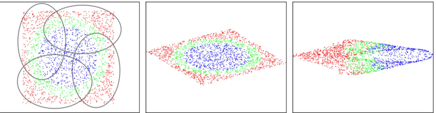
Figure 1. Synthetic dataset with color coded class labels, and the GMM used by our CLML local metric (left). Data projection given by a global Mahalanobis metric (middle) and our local CLML metric (right). The pairwise training constraints are better respected by CLML.
they minimize the Locally Linear Embedding (LLE) [30] objective function. Our work differs in that we learn co-ordinated local linear projections in a supervised manner. Also, in our work we use a diagonal covariance GMMs — which are faster to train than MFA— and learn local linear maps directly from the original feature space to the global representation instead of mapping from the local MFA sub-spaces. Since the MFA is learned by optimizing a different cost function, the obtained subspaces might be suboptimal.
3. Globally aligning local Mahalanobis metrics
Since any positive definiteD×DmatrixM can be de-composed as M = L>L, the Mahalanobis distance be-tween two pointsxiandxjcan be written as the`2distance
between these points after projection withL,i.e.
(xi−xj)>M(xi−xj) =kLxi−Lxj k22. (1)
Note thatLcan be aD×Dmatrix, or ad×Dmatrix with
d < D. In the latter case(Lxi)∈IRdis a low dimensional
projection ofxi∈IRD, and rank(M)≤d.
To obtain a more general class of metrics, we define sev-eral local Mahalanobis metrics. We cluster the data using a
k-component Gaussian mixture model (GMM), which de-fines a soft-assignment of the data over thekclusters.
We can compute distances between points assigned to the same clustersusing a local metric learned for that clus-ter, defined by a local projection matrixLs. It is, however,
not clear how to compare vectors that are assigned to dif-ferent clusters. In order to combine the local metrics, we define a global representation in which we integrate the lo-cal projections given by the differentLs. Similar to global
Mahalanobis metric learning, and unlike previous work, our formulation amounts to projecting the data (in a locally lin-ear way) to a new representation, and computing the`2
met-ric in this new representation. This allows us to compute distances between any pair of samples, regardless of their cluster assignments.
Figure1gives an illustration on a synthetic dataset. The dataset (left panel) is constructed in such a way that a global
linear projection cannot bring all points of each class close together, while keeping points of different classes apart. This is observed in the data projected using a global Maha-lanobis metric (middle panel). Using our “coordinated local metric learning” (CLML) approach, which we describe be-low, we obtain a data representation that respects the pair-wise training constraints much better (right panel).
3.1. Coordinated local metric learning
As pointed out above, we can interpret a Mahalanobis metric as computing the`2 distance after linear projection
of the data. Local Mahalanobis metrics can therefore be interpreted as locally mapping the data pointsxto several different, local, coordinate systems via projectionsLsx.
Since the`2 metric is invariant to translation, rotation,
and reflection of the coordinates, we can arbitrarily modify the projection ofxito a local coordinate system to
zis:=RsLsxi+bs, (2)
where Rs denotes an orthonormal matrix, i.e. for which
R>sRs=I, which can implement rotations and reflections,
andbsdenotes a translation. Using these transformations
we can coordinate the local projections so that they align across different local models. In particular, given that xi
andxjare assigned to different clustersrandtrespectively,
we can set the{Rs, bs}to ensure thatzirandzjtare close
ifxiandxj form a positive pair, and far away if they form
a negative pair.
Instead of learning the {Rs, bs} for fixedLsthat were
learned in advance, we will learn both the local metrics and their alignment in a joint manner. To that end, we can ab-sorbRsintoLswithout loss of generality, and define a
map-ping of the data pointsxito a global coordinate system as
zi:= k X s=1 qiszis= k X s=1 qis Lsxi+bs , (3)
whereqis :=p(s|xi)is the soft-assignment ofxito cluster
projection of the cluster to which it is assigned. In the case of soft-assignments,ziis the weighted average of the local
projections to the global representation. Our goal is now to learn{Ls, bs}so thatziandzjare close for positive pairs,
and far away for negative pairs. We assume the GMM clus-tering is fixed.
Note that we can re-write this weighted average of lo-cally linear projections as a single linear projection
zi = ˜Lx˜i, (4)
where L˜ = (L1, b1, . . . , Lk, bk) collects the local linear
projections, and x˜i = qi1(xi>,1), . . . , qik(x>i ,1)
> con-tainskcopies ofxiappended with a one, each weighted by
the corresponding soft-assignment. The projection matrixL˜
defines the local metrics used to compare points that are as-signed to the same cluster, but also the rotations, reflections, and translations to globally align the local representations.
For a given partitioning of the data, thezi are obtained
as a linear projection of the transformed input vectorsx˜i,
the`2distance betweenziandzjis therefore equivalent to
a Mahalanobis distance betweenx˜iandx˜j. The problem of
learning a globally aligned ensemble of local metrics there-fore takes the same form of learning a global Mahalanobis metric; be it using the expanded high-dimensional data rep-resentation given by the x˜i. As a result, existing
Maha-lanobis metric learning methods can be used to learn the projection matrixL˜for CLML.
It is easy to see that CLML generalizes Mahalanobis metrics. Fork ≥ 1, if each cluster suses the same pro-jection given byLs = L andbs = b, then for arbitrary
soft-assignmentszi =Lxi+bis a linear projection ofxi,
and the`2distance betweenziandzjis a Mahalanobis
dis-tance betweenxi andxj given byk L(xi−xj) k2. With
proper regularization, we therefore expect performance that is at least on par with global metric learning.
3.2. Implementation
Optimization. We use the LDML [15] objective func-tion to learn our local metrics parameterized byL˜. Let the labelyij ∈ {−1,+1}denote whether(xi, xj)is a positive
or a negative pair. LDML then minimizes the log-loss
L( ˜L, b) =X i,j
ln
1 + exp −yij(b− ||zi−zj||2) ,(5)
wherebis a scalar (estimated along withL˜) that determines at which distance pairs are considered positive or negative. We add a Frobenius norm regularizer overL˜ to avoid over-fitting, and cross-validate the regularization weight. We use a global LDML metric to initialize the local metrics.
In our implementation we use the sum formulation of Eq. (3), which avoids explicitly storing thex˜i. Compared
to global metric learning, we only need to additionally store
the soft-assignments. In practice this is a negligible over-head, in addition the assignments can be thresholded to be sparse. The cost to compute the zi increases sub-linearly
withkbecause of this sparsity.
Clustering. To partition the input space in CLML, we learn diagonal covariance GMMs. In our experiments we consider two alternatives for the data on which the GMMs are learned. We either learn the mixture in the original fea-ture space, or learn the mixfea-ture in the projection space ob-tained by global LDML metric learning. The rationale for the latter option is that the GMM clustering will be more meaningful in the global metric learning space.
Efficient retrieval.For efficient face retrieval we use the multiple assignment approach of [21]. Theziin the retrieval
set are clustered using k-means, and eachzi is assigned to
the nearest center. A queryzis assigned to themclosest k-means centers. Only points assigned to thesemcenters are returned, ranked by their distances to the queryz.
4. Experimental Evaluation
4.1. Dataset, protocols, and features
For our experiments we use the Labeled Faces in the Wild (LFW) [19] dataset. It contains a total of 13,233 faces of 5,749 people collected from the web. The dataset was designed for verification experiments, where we have to de-termine for a pair of face images if they depict the same person or not. In our experiments, we use the standard “un-restricted” training protocol, that allows the use of all pairs in the training set. The verification accuracy is measured us-ing ten-fold cross-validation. The train set is used to learn a metric, and to estimate a threshold on the metric. Using these, the pairs in the test set is classified as positive or neg-ative, and the accuracy of this classification is reported.
Since the LFW verification accuracy is saturating in re-cent years [24], we focus on the more challenging retrieval-based evaluation of Bhatterai et al. [3]. The set of 423 queries consists one image of each person in LFW with five or more images. All images not in the query set form the re-trieval set, and are used to learn the metric. We augment the retrieval set with up to one million distractor faces provided by Bhatteraiet al., which belong to people not present in the LFW dataset. The 1-call@n performance measure is the fraction of queries for which at least one of the top n
ranked result faces is of the same person. We also use the mean average precision (mAP) measure, which gives us a single number per setting instead of a full 1-call@ncurve.
We align face images with a similarity transform based on detection of points on the eyes, nose, and mouth, see [11]. We consider three representations. The first is the LBP features of Bhattaraiet al. [3], which allows direct comparison to their work. We compute a 9,860 dimensional descriptor by concatenating 58 dimensional LBPs [28] on
GMM feature space Nr. of local metricsk Original Global metric
2 73.04 73.09
4 74.04 75.18
6 73.58 75.24
8 73.92 75.59
Table 1. Evaluation of CLML over FV features using different GMM clustering methods. Performance is measured in mAP.
each cell of a 10×17grid over the face. The second is similar to the Fisher vector (FV) features of Simonyan et al. [35]. We densely compute at each pixel a root-SIFT descriptor [1], using 24×24 pixel patches. The descrip-tors are projected to 64 dimensions using PCA. Spatial lay-out information is incorporated by appending the 2D im-age coordinates of the patch center to the descriptors [31], providing a 66 dimensional local feature. We represent the face by computing a 16,896 dimensional FV [32] us-ing 128 Gaussian components. The third feature is derived from the penultimate layer of a convolutional neural net-work trained on the CASIA WebFace dataset [42], which contains 494,414 faces of 10,575 subjects. The network architecture is similar to the one proposed in [42] and the dimensionality of the extracted feature is 320.
4.2. Experimental evaluation results
For comparability with Bhattaraiet al. [3], we use pro-jections tod= 32dimensions unless stated otherwise.
Comparison of CLML with global metric learning.In Table1we compare CLML using GMMs trained either in the original FV features, or on data projected tod= 32 di-mensions by a global LDML metric,c.f. Section3.2. In all cases, the clustering obtained LDML projections leads to better results. Where the difference between the two clus-tering approaches is only 0.05 fork = 2local metrics, it increases for larger numbers of clusters, up to 1.67 fork= 8
local metrics. In all subsequent experiments we therefore use clustering using LDML projections. Clustering in the LDML projected space is also much faster: in this case it takes about 0.5 secs. to learn the GMM on 10,000 points.
In Table 2 we evaluate CLML on the three features, while varying the number of local metrics. We also state results obtained when cross-validating the number of local metrics, as well as results of global LDML metrics and the
`2metric. The results lead to the following observations. (i)
CLML generally improves when using more local metrics. (ii) Cross-validation over the number of local metrics suc-cessfully selects a (near) optimal number of local metrics. In subsequent experiments we cross-validate the number of local metrics for CLML. (iii) The FV features lead to better results than the LBP and CNN features. (iv) For all tested
Features Nr. local metricsk LBP FV CNN 2 41.51 73.09 59.78 4 44.02 75.18 61.43 8 47.94 75.59 64.64 16 49.00 76.20 66.07 32 49.98 75.61 70.98 64 49.70 75.58 73.83 Cross-validated 49.89 (26) 74.99 (28) 73.83 (64) Global LDML metric 36.95 68.12 58.46 `2metric 13.24 22.88 63.06
Table 2. Performance of CLML in retrieval mAP for the three fea-tures, while varying the number of local metrics.
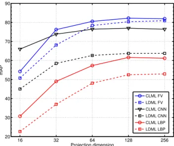
16 32 64 128 256 20 30 40 50 60 70 80 90 Projection dimension mAP CLML FV LDML FV CLML CNN LDML CNN CLML LBP LDML LBP
Figure 2. Performance in mAP of local and global metrics for the three features, using projection dimensions from 16 to 256.
settings, CLML consistently improves over LDML. In Figure2we compare CLML and LDML for the three features across a range of projection dimensions. The re-sults show that CLML consistently improves over LDML for all projection dimensions with the three features. The improvements are particularly large for the CNN and LBP features. For the LBP and FV features, the best results are obtained with CLML at d = 128, withk = 16 set by cross-validation: 61.6% and 82.2% mAP respectively. LDML with the same number of parameters,i.e. withd=
128×16 = 2048, obtains 53.0% and 80.9% respectively.
This shows that the improvement of CLML is not simply because it has more parameters. In the case of CNN de-scriptors, the best performance is obtained with CLML at
d= 128andk= 64set by cross-validation: 76.95% mAP.
Since the descriptors are only 320 dimensional, we cannot compare to LDML with the same number of parameters.
10 20 30 40 50 60 70 80 90 100 30 40 50 60 70 80 90
Number of retrieved results (n)
1−call @ n Zero distractors CLML, k=16 LDML Flat clustering, k=8 Hierarchical clustering, 256D4 [4] Hierarchical clustering, 256D4 [4] PCCA SCML 3 3 10 20 30 40 50 60 70 80 90 100 20 30 40 50 60 70
Number of retrieved results (n)
1−call @ n
With 100k distractors
Figure 4. Retrieval using LFW images only (left), and using LFW plus 100,000 distractor faces (right). The results marked with [3] correspond to those reported therein. Results for SCML and LDML have been produced using publicly available code. See text for details.
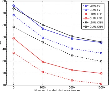
0 100k 500k 1000k 10 20 30 40 50 60 70 80
Number of added distractor images
mAP LDML FV CLML FV LDML LBP CLML LBP LDML CNN CLML CNN
Figure 3. Performance of CLML and LDML with different num-bers of distractors added to the LFW images.
Using a full-rank320×320Mahalanobis metric, however, yields 63.71% mAP, which is significantly worse.
Large-scale face retrieval experiments. In our second set of retrieval experiments we add up to one million addi-tional distractor images to the LFW images.
In Figure3we evaluate the results of CLML and LDML for the three features, while increasing the number of dis-tractors from zero to one million. We observe that per-formance degrades gracefully, and that the improvement of CLML over LDML is stable as a function of the number of distractors for all three features.
In Figure 4 we make a direct comparison to Bhattarai et al. [3]: re-plotting the 1-call@n curves reported there. From the other state-of-the-art methods discussed in Sec-tion2we compare to SCML [34].1 For LMLML [4] code
1Code available athttp://mloss.org/software/view/553.
is not available, while for R2LML [20] we found the code too inefficient to use with our high dimensional features.
For Bhattarai et al. we report the results for their “256D4” setting, which they found to give best results and uses eight local metrics, and also include their global met-ric learning results obtained with PCCA [25]. Our CLML results substantially improve over the results of Bhattaraiet al.,e.g. from under 40% to over 70% 1-call@nforn= 10
for the case without distractors (Figure4, left panel). Inter-esting we also obtained large improvements over Bhattarai et al. using global LDML metrics.
To understand the large performance difference, we re-implemented their approach (Figure 4, left panel, green curve), and obtained improvements of about 10 points w.r.t. their results. We found that most of this improvement is due to the`2regularization that we use, but Bhattaraiet al. did
not. We also implemented a non-hierarchical variant of their approach, based on “flat” k-means clustering, but which is otherwise the same (Figure4, left panel, black curve). This leads to another improvement of about 10 points, which suggests that flat clustering leads to clusters that are better suited for retrieval. Our global metric learning results ob-tained with LDML (Figure4, left panel, red dashed curve) are yet another 10 points better. This shows that the benefit of using local metrics is counterbalanced by only retrieving points assigned to the same cluster as the query, as is done by Bhattaraiet al. and for the green and black curves.
Using SCML [34] we obtained the worst retrieval results. This is because SCML learns metrics using a limited set of base metrics, which is detrimental for high-dimensional data. To improve results we tuned the number of base met-rics (600 gave best results), and also excluded faces of peo-ple with less than 3 images to compute the base metrics with FLDA, which also improved the results. The number of clusters used to produce the base metrics in SCML is an-other hyper-parameter that might require further tuning.
10−3 10−2 10−1 100 20 25 30 35 40 45
Relative number of distance computations
mAP GMM, 16 K−means, 16 K−means, 64 K−means, 256 K−means, 1024
Figure 5. Retrieval mAP and speed on LFW plus one million dis-tractor faces, using CLML withd= 32and FV feaures. Varying the number of quantization cellsp, and number of assignmentsm.
Efficient retrieval with CLML metrics. CLML projects all data in a single representation in which the`2
distance is used. Therefore we can decouple the cluster-ing used for local metric learncluster-ing, and the clustercluster-ing used for the efficient quantization-based multiple-assignment re-trieval method discussed in Section3.2.
In Figure 5 we consider the trade-off between the re-trieval mAP and search speed. The speed is measured as number of distance computations relative to the number needed for exhaustive search. Each curve shows, for a quan-tization intopcells, the performance using multiple assign-ment to m = 1,2,4, . . . , p clusters, where m= 1 corre-sponds to the lower-left point of each curve.
The blue curves show performance using 16 clusters: either using a k-means clustering computed over the zi
(solid), or using the GMM clustering used for the local metrics (dashed). Using the GMM clustering (dashed blue curve), a speedup factor 10 relative to exhaustive search can be achieved by single assignment (m= 1), but at the cost of a drop of around 10 points in mAP. Using k-means cluster-ing over thezi(solid blue curve) we obtain larger speedups
and higher mAP values. The results show that it is more ef-fective to dissociate the clustering used for the local metrics from the one used for retrieval, unlike the approach taken by Bhattaraiet al. [3].
Moreover, dissociating the clusterings, allows more flex-ibility in choosing the speed-vs.-accuracy operating point. By using k-means clustering with more than16centers we can substantially improve the search results: as seen by the red, black, and green curves forpequal to64,256, and1024
respectively. For example, with p= 1024clusters (green curve) and assignment tom= 64clusters we can reduce the search time by a factor 14, without compromising the mAP.
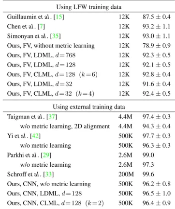
Using LFW training data
Guillauminet al. [15] 12K 87.5±0.4
Chenet al. [7] 12K 93.2±1.1
Simonyanet al. [35] 12K 93.0±1.1
Ours, FV, without metric learning 12K 78.9±0.9
Ours, FV, LDML,d= 768 12K 92.3±0.5
Ours, FV, LDML,d= 128 12K 92.1±0.5
Ours, FV, CLML,d= 128 (k= 6) 12K 92.8±0.4
Ours, FV, LDML,d= 32 12K 91.6±0.4
Ours, FV, CLML,d= 32 (k= 4) 12K 92.4±0.5 Using external training data
Taigmanet al. [37] 4.4M 97.4±0.3
w/o metric learning, 2D alignment 4.4M 94.3±0.4
Yiet al. [42] 500K 97.7±0.3
w/o metric learning 500K 96.3±0.3
Parkhiet al. [29] 2.6M 99.0
w/o metric learning 2.6M 97.3
Schroffet al. [33] 200M 99.6
Ours, CNN, w/o metric learning 500K 96.2±0.8
Ours, CNN, LDML,d= 128 500K 96.5±1.0
Ours, CNN, CLML,d= 128 (k= 2) 500K 96.4±0.9 Table 3. Comparing CLML using FV features with other metric learning methods. Performance as LFW verification accuracy.
Our speedup is comparable to the factor of 10 reported by Bhatteraiet al. [3] for 16 clusters in their hierarchical ap-proach, but our approach leads to better retrieval results.
Withp= 1024andm= 8, a speedup factor larger than 100
can be obtained while loosing less than 5 mAP points.
Face verification experiments. In Table3we compare our results obtained using local CLML metrics and global LDML ones to the state-of-the-art using the LFW face ver-ification evaluation.
When using no outside training data, the results of Chen et al. [7] (93.2±1.1) and Simonyanet al. (93.0±1.1) are sate-of-the-art. Using the`2metric as a baseline we obtain
78.9±0.9, which is improved using global LDML metrics
to 92.1±0.5 and 91.6±0.4 for d = 128 andd = 32
dimensional projections respectively. For both projection dimensions, CLML improves over LDML, to 92.8±0.4
and92.4±0.5respectively. We also observe a consistent improvement when comparing LDML (d= 128 andd= 768) with CLML (d= 32, k= 4andd= 128, k= 6) using the same number of parameters. This underlines once more that the improvements by CLML are not simply due a larger number of parameters.
Our results differ slightly from those of Simonyanet al. [35] due to a more efficient implementation: (i) They used GMMs with 512 components for the FV, while we use only
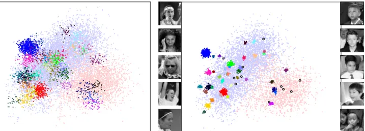
Figure 6. Visualization of the data projections learned by LDML (left) and CLML (right). Data points of the 40 most frequent people in the dataset have been color coded. Other data points are plotted in blue and pink for males and females respectively. On the sides of the CLML visualization we show outliers faces (marked with black circles) of males in the female cluster (right), and vice-versa (left). Interestingly, male outlier faces are mostly young boys, while female outlier faces mostly display extreme poses or expressions. Best viewed on screen.
128, yielding4×smaller descriptors. (ii) They average over left-right flipped versions of face image which we do not. (iii) Besides a Mahalanobis metric, they also learn a sim-ilarity of the form xT
iM xj, which they average with the
Mahalanobis metric, similar to Caoet al. [6].
In the bottom part of Table3we report results obtained using CNN features. Using the CNN features with the `2
metric we obtain96.2±0.8verification accuracy, similar to the results of Yiet al. [42] (96.3±0.3) which used the same training data for their network. Surprisingly, using our CNN descriptors we found that metric learning, either with LDML or CLML, gives only small improvements over the`2 baseline. The reason for this might be that the
per-formance of the `2 distance over the CNN features is
al-ready very high for the face verification task, or that the pair-wise loss function of LDML is less suitable for verifi-cation than the triplet-based loss used by Parkhiet al. [29], or the weighted chi-squared metric used by Taigmanet al. [37]. Yiet al. [42] used a multi-task learning objective to train their CNN jointly for both verification and recognition. The quoted results from the literature other than [42], are using CNNs trained on datasets that are 5 to 400 times larger, and therefore not directly comparable. Taigman et al. [37] use 4.4 million images and combine the output of three different CNNs and use 3D face alignment. Us-ing only 2D aligned images (as we do in our work), they reported slightly worse than ours before metric learning (94.3 ±0.4). Parkhi et al. [29] recently reported results using a deeper convolutional architecture [36] and 2D face alignment over 2.6 million images (99.0). The state of the art results of Schroffet al. [33] are based on an extremely large proprietary dataset of 200 million images, for which no alignment was used.
Data visualization. To illustrate the benefit of CLML
for data visualization we plot LFW images projected using CLML and LDML in Figure6. We learnedd= 256 dimen-sional projections on the FV features, and map these to 2D by PCA. For CLML the number of local metrics was set to
k= 12by cross-validation. CLML leads to a much better separation of the faces of different people, despite the lim-ited improvement of CLML (81.9) over LDML (80.8) in mAP ford= 256. Using CLML we can more clearly see the two groups corresponding to male and female faces. We used the LFW gender labels from the BeFIT website.2
5. Conclusion
We have presented our coordinated local metric learning (CLML) approach which learns local Mahalanobis metrics, and integrates them in a global representation where the`2
distance is used. This allows data visualization in a sin-gle view, and the use of efficient`2-based retrieval
meth-ods. Our low-dimensional global representation is obtained as a linear projection of an expanded data representation, defined using the input data and a Gaussian mixture clus-tering. We have presented results of extensive face retrieval and verification experiments on the Labeled Faces in the Wild dataset. In all settings CLML improves over global LDML metrics, or gives comparable results. For face re-trieval we obtain substantial improvements over global met-rics and previously reported local metric learning results. Our approach also allows efficient multiple-assignment re-trieval, which gives a better speed-accuracy trade-off than earlier work for face retrieval in a large-scale dataset with a million distractor faces.
References
[1] R. Arandjelovic and A. Zisserman. Three things everyone should know to improve object retrieval. InCVPR, 2012. [2] A. Bellet, A. Habrard, and M. Sebban. A Survey on Metric
Learning for Feature Vectors and Structured Data. ArXiv e-prints, 1306.6709, 2013.
[3] B. Bhattarai, G. Sharma, F. Jurie, and P. P´erez. Some faces are more equal than others: Hierarchical organization for ac-curate and efficient large-scale identity-based face retrieval. InECCV Workshops, 2014.
[4] J. Bohn´e, Y. Ying, S. Gentric, and M. Pontil. Large margin local metric learning. InECCV, 2014.
[5] J. Bromley, I. Guyon, Y. LeCun, E. Sackinger, and R. Shah. Signature verification using a siamese time delay neural net-work. InNIPS, 1993.
[6] Q. Cao, Y. Ying, and P. Li. Similarity metric learning for face recognition. InICCV, 2013.
[7] D. Chen, X. Cao, F. Wen, and J. Sun. Blessing of dimension-ality: high dimensional feature and its efficient compression for face verification. InCVPR, 2013.
[8] S. Chopra, R. Hadsell, and Y. LeCun. Learning a similarity metric discriminatively, with application to face verification. InCVPR, 2005.
[9] J. Davis, B. Kulis, P. Jain, S. Sra, and I. Dhillon. Information-theoretic metric learning. InICML, 2007.
[10] A. Dosovitskiy, J. Springenberg, M. Riedmiller, and T. Brox. Discriminative unsupervised feature learning with convolu-tional neural networks. InNIPS, 2014.
[11] M. Everingham, J. Sivic, and A. Zisserman. Taking the bite out of automatic naming of characters in TV video. Image and Vision Computing, 27(5):545–559, 2009.
[12] A. Frome, Y. Singer, F. Sha, and J. Malik. Learning globally-consistent local distance functions for shape-based image re-trieval and classification. InICCV, 2007.
[13] Z. Ghahramani and G. Hinton. The EM algorithm for mix-tures of factor analyzers. Technical Report CRG-TR-96-1, University of Toronto, May 1996.
[14] A. Globerson and S. Roweis. Metric learning by collapsing classes. InNIPS, 2006.
[15] M. Guillaumin, J. Verbeek, and C. Schmid. Is that you? Metric learning approaches for face identification. InICCV, 2009.
[16] M. Guillaumin, J. Verbeek, and C. Schmid. Multiple instance metric learning from automatically labeled bags of faces. In ECCV, 2010.
[17] S. Hauberg, O. Freifeld, and M. Black. A geometric take on metric learning. InNIPS, 2012.
[18] Y. Hong, Q. Li, J. Jiang, and Z. Tu. Learning a mixture of sparse distance metrics for classification and dimensionality reduction. InICCV, 2011.
[19] G. Huang, M. Ramesh, T. Berg, and E. Learned-Miller. La-beled faces in the wild: a database for studying face recogni-tion in unconstrained environments. Technical Report 07-49, University of Massachusetts, Amherst, 2007.
[20] Y. Huang, C. Li, M. Georgiopoulos, and G. Anagnostopou-los. Reduced-rank local distance metric learning. InECML, 2013.
[21] H. J´egou, M. Douze, and C. Schmid. Product quantization for nearest neighbor search.PAMI, 33(1):117–128, 2011. [22] M. K¨ostinger, M. Hirzer, P. Wohlhart, P. Roth, and
H. Bischof. Large scale metric learning from equivalence constraints. InCVPR, 2012.
[23] B. Kulis. Metric learning: A survey.Foundations and Trends in Machine Learning, 5(4):287–364, 2012.
[24] S. Liao, Z. Lei, D. Yi, and S. Li. A benchmark study of large-scale unconstrained face recognition. InInternational Joint Conference on Biometrics, 2014.
[25] A. Mignon and F. Jurie. PCCA: A new approach for distance learning from sparse pairwise constraints. InCVPR, 2012. [26] Y.-K. Noh, B.-T. Zhang, and D. Lee. Generative local metric
learning for nearest neighbor classification. InNIPS, 2010. [27] E. Nowak and F. Jurie. Learning visual similarity measures
for comparing never seen objects. InCVPR, 2007.
[28] T. Ojala, M. Pietik¨ainen, and T. M¨aenp¨a¨a. Multiresolution gray-scale and rotation invariant texture classification with local binary patterns.PAMI, 24(7):971–987, 2002. [29] O. Parkhi, A. Vedaldi, and A. Zisserman. Deep face
recog-nition. InBMVC, 2015.
[30] S. Roweis and L. Saul. Nonlinear dimensionality reduc-tion by locally linear embedding.Science, 290(5500):2323– 2326, 2000.
[31] J. S´anchez, F. Perronnin, and T. de Campos. Modeling the spatial layout of images beyond spatial pyramids. Pattern Recognition Letters, 33(16):2216–2223, 2012.
[32] J. S´anchez, F. Perronnin, T. Mensink, and J. Verbeek. Image classification with the Fisher vector: Theory and practice. IJCV, 105(3):222–245, 2013.
[33] F. Schroff, D. Kalenichenko, and J. Philbin. Facenet: A uni-fied embedding for face recognition and clustering. 2015. [34] Y. Shi, A. Bellet, and F. Sha. Sparse compositional metric
learning. InAAAI, 2014.
[35] K. Simonyan, O. Parkhi, A. Vedaldi, and A. Zisserman. Fisher vector faces in the wild. InBMVC, 2013.
[36] K. Simonyan and A. Zisserman. Very deep convolu-tional networks for large-scale image recognition. CoRR, abs/1409.1556, 2014.
[37] Y. Taigman, M. Yang, M. Ranzato, and L. Wolf. DeepFace: Closing the gap to human-level performance in face verifica-tion. InCVPR, 2014.
[38] Y. Teh and S. Roweis. Automatic alignment of local repre-sentations. InNIPS, 2003.
[39] J. Wang, A. Kalousis, and A. Woznica. Parametric local metric learning for nearest neighbor classification. InNIPS, 2012.
[40] J. Wang, K. Sun, F. Sha, S. Marchand-Maillet, and A. Kalousis. Two-stage metric learning. InICML, 2014. [41] K. Weinberger and L. Saul. Distance metric learning for
large margin nearest neighbor classification.JMLR, 10:207– 244, 2009.
[42] D. Yi, Z. Lei, S. Liao, and S. Li. Learning face representation from scratch. InArxiv preprint, 2014.
[43] D.-C. Zhan, M. Li, Y.-F. Li, and Z.-H. Zhou. Learning in-stance specific diin-stances using metric propagation. InICML, 2009.