Efficient Reliability and Sensitivity Analysis of Complex Systems and Networks with Imprecise Probability

Efficient Reliability and Sensitivity Analysis of

Complex Systems and Networks with Imprecise

Probability

Thesis submitted in accordance with the requirements of

the University of Liverpool for the degree of Doctor in Philosophy

by

Geng Feng

Declaration

I hereby declare that except where specific reference is made to the work of others, the contents of this dissertation are original and have not been submitted in whole or in part for consideration for any other degree or qualification in this, or any other university. This dissertation is my own work and contains nothing which is the outcome of work done in collaboration with others, except as specified in the text and Acknowledgements. This dissertation has 145 pages, 60 figures, 23 tables and 48062 words.

Geng Feng May 2017

Acknowledgement

My main appreciation and first greatest acknowledgements to my supervisors Professor Michael Beer and Dr Edoardo Patelli. Michael Beer’s ultimate support and guidance have been crucial to expand my academic horizon and take my research forwards step by step. Also, his gracious and generous personality is an example for me to learn from and makes my doctoral experience rather unique. I am very grateful to him.

Edoardo Patelli has given me constant and specific guidance during my PhD studies. I appreciate his high standards, his knowledge of research methodologies and his talented ability for software. His willingness and invaluable suggestions highly improve my dis-sertation. The years working with him have made my doctorate very prolific, enjoyable and unique, so I appreciate him from my heart.

I am extremely grateful to Professor Frank P.A. Coolen, who has pointed out a clear academic direction for me in the research ocean. His strong mathematical and systematic knowledge impresses me a lot, and he has taught me patiently and without reservation. It is really hard to find the words to express my gratitude and appreciation for him.

I very much acknowledge Dr Sean Reed and Dr Marco de Angelis’s help, as their understanding of computational analysis and software development helped me a lot as a PhD researcher. Many sincere thanks to my close friend Hindolo George-Williams for his inreplaceable help and efficient cooperation during my PhD. Special thanks to Professor David Percy and Dr Anas Batou for their useful comments on this thesis.

I am also pretty grateful to the Institute for Risk and Uncertainty, which provided the perfect and friendly environment for my research. My deep appreciation goes out to Professor Scott Ferson, Dr Louis Aslett, Dr David Opeyemi, Dr Raphael Moura, Dr Oscar Nieto-Cerezo, Dr Matteo Broggi, Ms Roshini Prasad, Uchenna Oparaji and other Institute members who played essential roles during my study.

My special thanks go to my parents who give me everything a son could wish for. Words cannot express how grateful I am to my mother and father for all of the sacrifices that they have made on my behalf. I want also to acknowledge my closest supporters, my beloved wife Danqing Li, for her meticulous care and constant encouragement, and my son Zeyou Feng, who lightens my life with his smiles and ever present love.

Abstract

Complex systems and networks, such as grid systems and transportation networks, are backbones of our society, so performing RAMS (Reliability, Availability, Maintainabil-ity, and Safety) analysis on them is essential. The complex system consists of multiple component types, which is time consuming to analyse by using cut sets or system signa-tures methods. Analytical solutions (when available) are always preferable than simulation methods since the computational time is in general negligible. However, analytical solu-tions are not always available or are restricted to particular cases. For instance, if there ex-ist imprecisions within the components’ failure time dex-istributions, or empirical dex-istribution of components failure times are used, no analytical methods can be used without resorting to some degree of simplification or approximation. In real applications, there sometimes exist common cause failures within the complex systems, which make the components’ independence assumption invalid.

In this dissertation, the concept of survival signature is used for performing reliability analysis on complex systems and realistic networks with multiple types of components. It opens a new pathway for a structured approach with high computational efficiency based on a complete probabilistic description of the system. An efficient algorithm for evaluating the survival signature of a complex system bases on binary decision diagrams is introduced in the thesis.

In addition, the proposed novel survival signature-based simulation techniques can be applied to any systems irrespectively of the probability distribution for the component fail-ure time used. Hence, the advantage of the simulation methods compared to the analytical methods is not on the computational times of the analysis, but on the possibility to analyse any kind of systems without introducing simplifications or unjustified assumptions. The thesis extends survival signature analysis for application to repairable systems reliability as well as illustrates imprecise probability methods for modelling uncertainty in lifetime distribution specifications.

Based on the above methodologies, this dissertation proposes applications for calcu-lation of importance measures and performing sensitivity analysis. To be specific, the novel methodologies are based on the survival signature and allow to identify the most

critical component or components set at different survival times of the system. The impre-cision, which is caused by limited data or incomplete information on the system, is taken into consideration when performing a sensitivity analysis and calculating the component importance index.

In order to modify the above methods to analyse systems with components that are subject to common cause failures,α-factor models are presented in this dissertation. The approaches are based on the survival signature and can be applied to complex systems with multiple component types. Furthermore, the imprecision and uncertainty within the

α-factor parameters or component failure distribution parameters is considered as well. Numerical examples are presented in each chapter to show the applicability and effi-ciency of the proposed methodologies for reliability and sensitivity analysis on complex systems and networks with imprecise probability.

List of Publications

Journal Papers:

• Feng G, Patelli E, Beer M, and Coolen F PA. Imprecise System Reliability and Com-ponent Importance based on Survival Signature, Reliability Engineering & System Safety, 2016, 150, 116-125

• Patelli E, Feng G, Coolen F PA, and Coolen-Maturi T. Simulation Methods for System Reliability Using the Survival Signature,Reliability Engineering & System Safety, 2017, 167, 327-337

Conference Papers:

• Feng G, Patelli E, and Beer M. Reliability Analysis of Systems Based on Survival Signature, International Conference on Applications of Statistics and Probability in Civil Engineering, 2015

• Feng G, Patelli E, and Beer M. Survival Signature-based Sensitivity Analysis of Systems with Epistemic Uncertainties, European Safety and Reliability Conference, 2015

• Feng G, Patelli E, and Beer M. Reliability Analysis of Complex Systems with Un-certainties by Monte Carlo Simulation Method, Asian-Pacific Symposium on Struc-tural Reliability and its Application, 2016

• Feng G, Patelli E, Beer M, and Coolen F PA. Component Importance Measures for Complex Repairable System, European Safety and Reliability Conference, 2016 • Patelli E, Feng G. Efficient Simulation Approaches for Reliability Analysis of Large

Systems. International Conference on Information Processing and Management of Uncertainty in Knowledge-Based Systems, 2016

• Beer M, Feng G, Patelli E, Broggi M, and Coolen F PA. Reliability Assessment of Systems with Limited Information, International Symposium on Reliability Engi-neering and Risk Management, 2016

• Feng G, Reed S, Patelli E, Beer M, and Coolen F PA. Efficient Reliability and Uncer-tainty Assessment on Lifeline Networks Using the Survival Signature, International Conference on Uncertainty Quantification in Computation Science and Engineering, 2017

• Feng G, Patelli E, Beer M, and Coolen F PA. Reliability Analysis on Complex Sys-tems with Common Cause Failures, International Conference on Structural Safety and Reliability, 2017

Contents

Declaration i

Acknowledgement iii

Abstract v

List of Publications vii

Contents xii

List of Figures xv

List of Tables xviii

1 Introduction 1

Introduction 1

1.1 Overview . . . 1

1.2 Problem Statement . . . 2

1.3 Aims and Objectives . . . 7

1.4 Structure of Thesis . . . 8

2 Theoretical Background 9 Theoretical Background 9 2.1 Introduction . . . 9

2.2 State Vector and Structure Function . . . 9

2.2.1 Component State Vector . . . 10

2.2.2 System Structure Function . . . 10

2.2.3 Relationship between State Vector and Structure Function . . . . 10

2.3.1 Simple System . . . 12 2.3.2 Parallel-Series System . . . 12 2.3.3 Non-Parallel-Series System . . . 13 2.4 Signature . . . 15 2.4.1 System Signature . . . 15 2.4.2 Survival Signature . . . 16 2.5 Numerical Tools . . . 19 2.5.1 R Package . . . 19

2.5.2 An Efficient Algorithm for Calculating Survival Signature of Com-plex Systems . . . 20

2.5.3 OpenCossan . . . 23

3 Complex System Reliability Analysis Based on Survival Signature 25 Complex System Reliability Analysis Based on Survival Signature 25 3.1 Introduction . . . 25

3.2 Reliability Assessment on Complex System with Multiple Component Types 26 3.3 Generalised Probabilistic Description of the Failure Times of Components 27 3.3.1 Introduction of Probability Box . . . 28

3.3.2 Analytical Method to Deal With Imprecision Within Components’ Failure Times . . . 29

3.3.3 Imprecise System . . . 32

3.4 Proposed Simulation Methods . . . 33

3.4.1 Algorithm 1 . . . 33

3.4.2 Algorithm 2 . . . 36

3.4.3 Simulation Method to Deal With Imprecision Within Components’ Failure Times . . . 39

3.5 Numerical Examples . . . 41

3.5.1 Circuit Bridge System . . . 41

3.5.2 Hydroelectric Power Plant System . . . 44

3.5.3 Grey System . . . 47

3.5.4 Complex Lifeline Network . . . 49

3.6 Conclusion . . . 53

4 Reliability Analysis of Complex Repairable Systems 55 Reliability Analysis of Complex Repairable System 55 4.1 Introduction . . . 55

4.2.1 Repairable System and Its Components . . . 56

4.2.2 Proposed Method for Repairable System Analysis . . . 56

4.3 Numerical Example . . . 58

4.3.1 Circuit Bridge System . . . 58

4.3.2 Complex System . . . 61

4.4 Conclusion . . . 63

5 Importance and Sensitivity Analysis of Complex Systems 67 Importance and Sensitivity Analysis of Complex System 67 5.1 Introduction . . . 67

5.2 Component Importance Measures of Non-repairable Systems . . . 68

5.2.1 Definition of Relative Importance Index . . . 68

5.2.2 Imprecision Within Relative Importance Index . . . 69

5.3 Component Importance Measures of Repairable Systems . . . 72

5.3.1 Importance Measure of a Specific Component . . . 73

5.3.2 Importance Measure of a Set of Components . . . 74

5.3.3 Quantify Importance Degree . . . 75

5.4 Sensitivity Analysis for Systems Under Epistemic Uncertainty with Prob-ability Bounds Analysis . . . 76

5.4.1 Represent Epistemic Uncertainty by P-box . . . 76

5.4.2 Probability Bounds Analysis as Sensitivity Analysis . . . 78

5.5 Numerical Example . . . 79

5.5.1 Hydroelectric Power Plant System . . . 79

5.5.2 Repairable Complex System . . . 81

5.5.3 Typical Complex System . . . 85

5.6 Conclusion . . . 89

6 Complex System Reliability Under Common Cause Failures 91 Complex System Reliability Under Common Cause Failures 91 6.1 Introduction . . . 91

6.2 System Reliability after Common Cause Failures . . . 92

6.2.1 Instruction ofα-factor Model . . . 92

6.2.2 Standardα-factor Model for System Reliability . . . 93

6.2.3 Generalα-factor Model for System Reliability . . . 94

6.2.4 Time Dependent System Reliability after CCFs . . . 95

6.2.5 Imprecise System Reliability after CCFs . . . 95

6.3.1 Case 1 (Standardα-factor Model) . . . 97

6.3.2 Case 2 (Generalα-factor Model One) . . . 98

6.3.3 Case 3 (Generalα-factor Model Two) . . . 99

6.3.4 Case 4 (Time Dependent System Reliability after CCFs) . . . 100

6.3.5 Case 5 (Imprecise System Reliability after CCFs) . . . 101

6.4 Conclusion . . . 103

7 Conclusion Remarks 105 Conclusions and Discussions 105 7.1 Conclusions . . . 105

7.2 Discussion and Future Work . . . 106

Appendix 109

Appendix 1: Survival Signature of System in Figure 3.17 109 Appendix 2: Survival Signature of System in Figure 4.9 127 Appendix 3: Values ofP(f1, f2, f3, f4)andΦ(l1, l2, l3, l4)of Case 1 in Chapter 6 130

Appendix 4: Past Data of System in Figure 6.1 132

List of Figures

2.1 Series system withmcomponents. . . 10

2.2 Parallel system withmcomponents. . . 11

2.3 Complex parallel-series system. . . 12

2.4 Complex non-parallel-series system. . . 13

2.5 A typical complex bridge system with two types of components: the num-ber outside the box is the component index, while the numnum-ber inside the box represents the component type. . . 18

2.6 A simple network with 4 nodes and 4 edges. . . 21

2.7 BDD for the simple network from Figure 2.6. . . 21

2.8 Algorithm for computing signature from the BDD representation of a sys-tem structure function. . . 22

3.1 All combinations of distributions for eventX. . . 29

3.2 P-box for eventX. . . 30

3.3 System with two types of components. . . 32

3.4 Flow chart of Algorithms 1-2. . . 38

3.5 A general schematic diagram for one simulation sample. . . 40

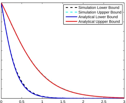
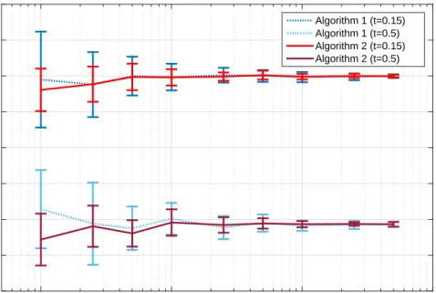
3.6 Lower and upper bounds of the survival function obtained by simulation and analytical method. . . 41

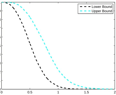
3.7 Lower and upper bounds of survival function by simulation method. . . . 42

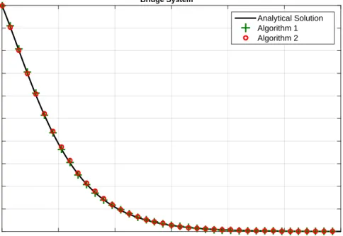
3.8 Survival function of the bridge system calculated by two simulation meth-ods and analytical method, respectively. . . 43

3.9 Example of a realization of the number of working components Ck as a function of time. . . 43

3.10 Standard deviation of the estimator of the survival function as a function of the number of samples. . . 44

3.11 Schematic diagram of a hydroelectric power plant system. . . 46

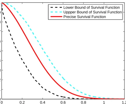
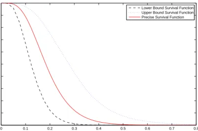
3.13 Survival function of a hydroelectric power plant system along with sur-vival functions for the individual components. . . 47 3.14 Upper, lower and precise survival functions of the hydroelectric power

plant system. . . 48 3.15 Grey system composed by 8 components of three types with imprecision

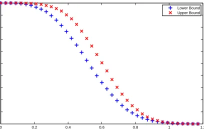
of the exact system configuration. . . 49 3.16 Upper and lower bounds of survival function for the system in Figure 3.15. 50 3.17 A lifeline network with 17 nodes and 32 edges. . . 50 3.18 Time varying precise survival function alongside with lower and upper

bounds of survival function of the network in Figure 3.17 (imprecise dis-tribution parameters). . . 53 3.19 Grey box of the network in Figure 3.17. . . 53 3.20 Lower and upper bounds of survival function of the network in Figure 3.17

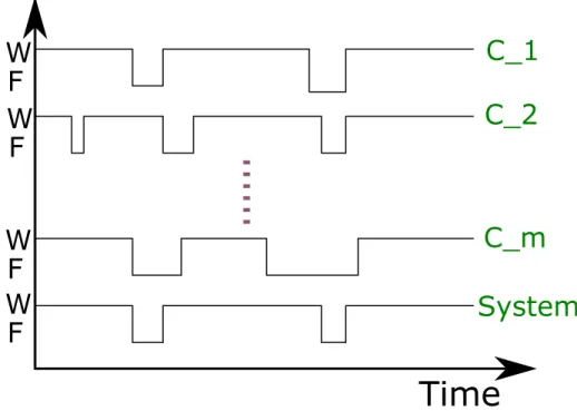
(imprecise survival signature). . . 54 4.1 Sketch map of a repairable component. . . 56 4.2 Schematic diagram of the repairable components status and the

corre-sponding system performance. . . 57 4.3 Flow chart of Algorithm 3. . . 60 4.4 Example of a realization of the number of working components Ck as a

function of time. . . 61 4.5 CASE A: Survival function of the circuit bridge system with repairable

components calculated by means of Algorithm 3 and a simulation method based on structure function. . . 62 4.6 CASE A: Standard deviation of the estimator for the circuit bridge system

with repairable components calculated by means of Algorithm 3 and a simulation method based on structure function. . . 62 4.7 CASE B: Survival function of the circuit bridge system with repairable

components calculated by means of Algorithm 3 and a simulation method based on structure function. . . 63 4.8 CASE B: Standard deviation of the estimator for the circuit bridge system

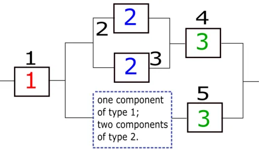
with repairable components calculated by means of Algorithm 3 and a simulation method based on structure function. . . 63 4.9 The complex repairable system with 14 components which belong to six

types. The numbers inside the component boxes indicate the component type. The numbers outside the component boxes indicate the component indices. . . 64 4.10 Survival function of the complex system calculated by Algorithms 1 and

4.11 Survival function of the complex system with repairable components. . . 65 5.1 Component 4 works at timet. . . 70 5.2 Component 4 fails at timet. . . 70 5.3 Relative importance index of Component 4 with precise distribution

pa-rameters. . . 72 5.4 Relative importance index of Component 4 with imprecise distribution

parameters. . . 73 5.5 Example of p-box of the system survival function . . . 77 5.6 Relative importance index values of the system components. . . 81 5.7 Upper and lower relative importance index of components CG, BV, T

andG. . . 82 5.8 Upper and lower relative importance index of componentsCB andT X. . 82 5.9 Relative importance index of the specific component in the system. . . 83 5.10 Relative importance index of the components sets with same type in system. 83 5.11 Relative importance index of the components sets with different types in

system. . . 84 5.12 Quantitative importance index of the specific component in the system. . . 85 5.13 Quantitative importance index of the components sets with different types

in the system. . . 85 5.14 Typical complex system: the number outside the box is the component

index, while the number inside the box represents the component type. . . 86 5.15 The bounds of imprecise survival function and precise survival function

of the typical system . . . 87 5.16 The p-box of the system survival function when component 1 is pinched

by a precise distribution . . . 87 5.17 The p-box of the system survival function when components set C[1,3] is

pinched by a precise distribution . . . 88 6.1 Complex system with thirteen components which belong to four types.

The number inside the component box represents the type, while the num-ber outside the box expresses the component index. . . 97 6.2 Survival functions of the system after some conditions’ common cause

failures. . . 101 6.3 Lower and upper survival function bounds of the system after the common

cause failures of C(0,0,1,1), C(0,2,0,2) and C(2,2,1,3) respectively. . . 102 6.4 Lower and upper survival function bounds of the system after the common

List of Tables

2.1 Ordered component failure times for the system in Figure 2.3. . . 16

2.2 Survival signature of the system in Figure 2.5 . . . 19

3.1 Survival signature of the bridge system of Figure 3.3 . . . 32

3.2 Imprecise distribution parameters of components in a system . . . 41

3.3 Failure types and distribution parameters of components in a hydro power plant . . . 45

3.4 Survival signature of a hydro power plant in Figure 3.11; rows withΦ(l1, l2, l3, l4, l5, l6) = 0are omitted . . . 45

3.5 Components failure types and distribution parameters for the system in Figure 3.15 . . . 48

3.6 Imprecise survival signature of the system of Figure 3.15,Φ(l1, l2, l3) = 0 andΦ(l1, l2, l3) = 1for both lower and upper bounds are omitted. . . 49

3.7 Survival signature of the network in Figure 3.17. . . 51

3.8 Failure types and imprecise distribution parameters of edges in the net-work of Figure 3.17. . . 52

4.1 Parameters of repairable components in the bridge system. State 1: Work-ing, State 2: Not-working. . . 61

4.2 Components failure (transition1 →2) and repair (transition2 →1) data for each component type of the complex system. . . 64

5.1 Survival signature of the system in Figure 5.1 . . . 71

5.2 Survival signature of the system in Figure 5.2 . . . 71

5.3 Component importance equations ofBM,RAW andF V . . . 79

5.4 Comparision of component importance obtained using different methods att= 0.12 . . . 80

5.5 Imprecise and precise distribution parameters of all components in the typical complex system . . . 86

6.2 Failure types and distribution parameters of components of the system in Figure 6.1 . . . 100 7.1 Survival signature of a complex network in Figure 3.17; rows withΦ(l1, l2, l3) =

0andΦ(l1, l2, l3) = 1are omitted . . . 109

7.2 Survival signature of a complex system in Figure 4.9; rows withΦ(l1, l2, l3, l4, l5, l6) =

0andΦ(l1, l2, l3, l4, l5, l6) = 1are omitted . . . 127

7.3 Values ofP(f1, f2, f3, f4)and their corresponding survival signatureΦ(l1, l2, l3, l4),

note thatfi =mi−li . . . 130

Chapter 1

Introduction

1.1

Overview

Reliability engineering deals with the construction and study of reliable systems. The first example of reliability calculation and estimation can be found in [1], which studied the probability for humans surviving to different ages. At the onset of World War II, with statistics theory and mass production well established, reliability engineering was ready to emerge [2].

Weibull proposed a statistical distribution function of wide applicability in [3], which is a standard tool for reliability applications. Birnbaum firstly put forward the importance measure in [4], which can be used to rank components in a system according to how important they are. Barlow and Proschan proposed the mathematical theory for reliability [5], which is one of the standard texts in the reliability engineering field.

Nowadays reliability engineering is used in a wide range of applications in complex systems and networks, which are series of components interconnected by communication paths. The analysis of these systems becomes more and more important as they are the backbones of our societies. Examples include the Internet, social networks of individu-als or businesses, transportation networks, power plant systems, aircraft and space flights, metabolic networks, and many others. Since the breakdown of a system may causes catas-trophic effects, it is essential to be able to assess the reliability and availability of these systems.

Uncertainty is an unavoidable component affecting the behaviour of systems and more so with respect to their limits of operation. In spite of how much dedicated effort is put into improving the understanding of systems, components and processes through the collection of representative data, the appropriate characterisation, representation, propagation and

interpretation of uncertainty will remain a fundamental element of the reliability analysis of any complex systems [6].

By studying the survival function of the complex systems and networks, the engineers can know the performance of them at different times. By using component importance measures, it is possible to draw conclusions about which component or components set is the most important to the whole system. By researching on the configuration and the lifetime of components, experts can design for reliability of the complex networks and systems. By considering uncertainty within the system, insights into the analysis outcomes can be produced which can be used meaningfully by decision-makers.

1.2

Problem Statement

The study of the reliability of complex systems, particularly systems with structures that cannot be sequentially reduced by considering alternative series and parallel subsystems, is a subject which has attracted much attention in the literature and which is of obvious im-portance in many applications [7]. A system is a collection of components whose proper function leads to the coordinated functioning of the system. In reliability analysis, it is therefore important to model the relationship between various items as well as the relia-bility of the individual components, to determine the reliarelia-bility of the system as a whole.

Traditionally, the reliability analysis of systems is performed adopting different well-known tools such as reliability block diagrams, fault tree and success tree methods, failure mode and effect analysis, and master logic diagrams [8]. The main limitation to applying these traditional approaches to large complex systems is the complex and tedious calcula-tions to find minimal path sets and cut sets.

In recent years, the system signature has been recognised as a useful tool to quan-tify the reliability of systems consisting of independent and identically distributed (iid) or exchangeable components with respect to their random failure times [9] [10]. It can be said that such systems only have “components of one type”. The system signature en-ables full separation of the system structure from the component probabilistic failure time distribution when deriving the system failure time distribution.

However, attempting to generalise the system signature to systems with more than one component type is not really possible as it requires the computation of the probabilities of different order statistics of the different failure time distributions involved [11], which tends to be intractable.

Most complex systems, such as automobiles, communication systems, aircraft, aircraft engine controllers, printers, medical diagnostics systems, helicopters, train locomotives, etc., are repaired and are not replaced when they fail [12]. To be specific, a complex

repairable system is a system that can be restored to an operating condition following a failure [13]. Similarly, the repairable components are those that are not replaced following the occurrence of a failure; rather, they are repaired and put into operation again. There-fore, it is essential to perform reliability analysis on complex repairable systems in the real application area.

Component importance measurement allows to quantify the importance of system components and identify the most “critical” component. It is a useful tool to find weak-nesses in systems and to prioritise reliability improvement activities. Birnbaum [4] pro-posed in 1969 a measure to find the reliability importance of a component, which is ob-tained by partial differentiation of the system reliability with respect to the given compo-nent reliability. An improvement or decline in reliability of the compocompo-nent with the highest importance will cause the greatest increase or decrease in system reliability. Several other importance measures have been introduced [14]. Improvement potential, risk achievement worth, risk reduction worth, criticality importance and Fussell-Vesely’s measure were all reviewed in Ref. [15] [16] [17] [18]. To conduct reliability importance of components in a complex system, Wang et al. [19] introduced and presented failure criticality index, restore criticality index and operational criticality index. Zio et al. [20] [21] presented generalised importance measures based on Monte Carlo simulation. The component im-portance measures can determine which components are more important to the system, which may suggest the most efficient way to prevent system failures.

However, the traditional importance measures mainly focus on non-repairable systems, and mainly concern reliability importance of individual components. In many practical situations it is of interest to evaluate the importance of a set of components instead of just an individual component.

Some of the importance measures can be computed through analytical methods, but limited to systems with few components. Traditional simulation methods provide no easy way to compute component importance [19]. In addition, in the case of imprecision in component failures, the simulation approaches become intractable.

As an intrinsic feature, practical systems involve uncertainties to a significant extent. Since the reliability and performance of systems are directly affected by uncertainty, a quantitative assessment of uncertainty is widely recognised as an important task in practi-cal engineering [22]. The obvious pathway to a realistic and powerful analysis of systems is a probabilistic approach.

Most existing models assume that there are precise parameter values available, so the quantification of uncertainty is mostly done by the use of precise probabilities [23]. How-ever, due to lack of perfect knowledge, imprecision within the component failure times or their distribution parameters can not be ignored. Hence, the sensitivity analysis for the whole system is affected by the epistemic uncertainty [24].

In order to deal with the uncertainty, the Dempster-Shafer approach to represent un-certainty was articulated by Dempster [25] and Shafer et al. [26]. Troffaes et al. [27] pre-sented a robust Bayesian approach to modelling epistemic uncertainty in common-cause failure models. Tonon [28] used random set theory to propagate epistemic uncertainty through a mechanical system. Helton et al. [29] combined sensitivity analysis with evi-dence theory to represent epistemic uncertainty. Fuzzy set theory is also proposed to deal with uncertainty in [30] [31]. An integrated framework to deal with scarce data, aleatory and epistemic uncertainties is presented by Patelli et al. [32], and OpenCossan is an effi-cient tool to perform uncertainty management of large finite element models [33].

On top of the above methods, Williamson and Downs [34] introduced interval-type bounds on cumulative distribution functions, which is called “probability boxes” or “p-boxes” for short. The use of p-boxes in risk analysis offers many significant advantages over traditional probabilistic approaches because it provides convenient and comprehen-sive ways to handle several of the most practical serious problems faced by analysts [35]. For example, Karanki et al. [36] expressed uncertainty analysis based on p-boxes in prob-abilistic safety assessment. Evidential networks for reliability analysis and performance evaluation of systems with imprecise knowledge was introduced by Simon and Weber [37]. In order to make a quantification of margins and uncertainties, Sentz and Ferson [38] presented probabilistic bounding analysis (PBA), which also can be used to perform the sensitivity analysis of systems. This approach represents the uncertainty about a prob-ability distribution by a set of cumulative distribution functions lying entirely within a pair of bounding distributions [39].

Dependence among failures might affect considerably the reliability of a system, and it is a relationship that causes multiple components to fail simultaneously, which exists widely in complex systems [40]. Dependence represents a common feature of compo-nent failures that needs to be modelled appropriately for a realistic analysis of systems and networks. The proper consideration and modelling of CCFs are essential in complex systems reliability analysis as they may have a large effect on the systems’ overall func-tionality. Often the assumption that the component failures are independent is considered in classical reliability analysis on systems. However, CCFs make this simplification not realistic. What is more, CCFs have been shown to decrease the reliability and availability of complex systems [41]. Therefore, common cause failures are extremely important in reliability assessment and must be given adequate treatment to minimise overestimation of systems’ performances.

A number of parametric models have been developed for common cause failures over the last decades. For instance, Rasmuson and Kelly [42] reviewed the basic concepts of modelling CCFs in reliability and risk studies. One of the most commonly used single parameter models defined by Fleming [43] is called theβ-factor model, which is the first

parameter model applied to common cause failures in risk and reliability analysis. Then, he generalised theβ-factor model to a multiple Greek letter model in 1986 [44]. Theα -factor model originally proposed by Mosleh et al. [45] develops CCFs from a set of failure ratios and the total component failure rate.

Recently, based on the α-factor model, Kelly and Atwood [46] presented a method for developing Dirichlet prior distributions that have specified marginal means. A robust Bayesian approach to modelling epistemic uncertainty in the imprecise Dirichlet model has been discussed by Troffaes et al. [27]. Coolen and Coolen-Maturi [47] present a non-parametric predictive inference for system reliability following common cause failures of components but limited to systems with exchangeable or a single type of components. Here, the work presented in Ref [47] is extended to perform reliability analysis on com-plex systems by considering CCFs among components belonging to different types; the proposed approach is based on the survival signature [48].

This dissertation mainly uses the survival signature methodology, which is associated with a survival analysis of systems [49]. Survival analysis has important applications in biology, medicine, insurance, reliability engineering, demography, sociology, economics, etc. In engineering, survival analysis is typically referred to as reliability analysis, and the survival function is then called reliability function. This survival function or reliability function quantifies the survival probability of a system at a certain point in time.

System signature has been recognised as an important tool to quantify the reliability of systems. However, the use of the system signature is associated with the assumption that all components in the system are of the same type.

Generally, in reliability problems for large-scale real-world systems and networks, simulation tools are required in order to provide reliability metrics. It is therefore impor-tant to put forward the efficient simulation methods which only use the survival signature. These methodologies do not need to use the entire structure function of the systems, which will provide a new insight into the system reliability.

Parameter uncertainties and imprecisions are generally epistemic in nature due to the lack of knowledge or data, or the unknown relationship between components (e.g., poor understanding of accident initiating events or coupled physics phenomena, lack of data to characterise experiment processes, random errors in measuring and analytic devices), all of them make it difficult to characterise probabilistically the failure time of components. Since the reliability and performance of systems are directly affected by uncertainties and imprecisions, a quantitative assessment of uncertainty is widely recognised as an important task in engineering [50].

Simulation approaches are used to investigate large and complex systems and to obtain numerical solutions where analytical solutions are not available. In particular, simulation methods allow the explicit consideration of the effect of uncertainty and imprecision on

the system under investigation, providing a powerful tool for risk analysis, which allows better decision making under uncertainty. Simulation methods can be used to identify problems before implementation, evaluate ideas, identify inefficiencies and understand why observed events occur.

The use of simulation methods for system reliability has many attractive features. Gen-erally, they can be used for the sensitivity analysis of multi-criteria decision models [51], to optimise models with rare events [52] and to perform multi-attribute decision making [53].

Most of the current simulation methods are based on Monte Carlo simulation and structure function. By generating the state evolution of each component, the structure function is computed to determine the state of the system. However, the calculation of the structure function usually requires the calculation of all the cut-sets and for large systems it is a challenging and error-prone task (see e.g. [54]). Moreover, the structure function is in a Boolean format and can only be used to identify a specific output of the system. Of course, more structure function can be used to match all the possible status of the system, at the cost of significantly increasing the time required by the analysis. Instead, the survival signature is a summary of the structure function, that is sufficient for basic reliability inferences (e.g. determining the system reliability function). In particular, for very large scale systems and networks, storing only the survival signature and not the entire structure function is clearly advantageous.

In a nutshell, in practical cases there are five specific challenges that need to be ad-dressed to obtain realistic results.

• First, the complexity of the system needs to be reflected in the numerical model. This goes far beyond a model based on a set of components with simple connections between them. For instance, there may be several different types of components in the same system. The variety of the components in the large size of real-life systems makes it difficult to predict the system lifetime and reliability, especially when they exit uncertainty characteristics.

• Second, when modelling failure time data, there is a distinction that needs to be made between one-time-use (or non-repairable) and multiple-time-use (or repairable) systems. When a non-repairable system fails, engineers simply replace it with a new system of the same type. In real engineering applications, however, there will be al-ways repairable complex systems to be analysed.

• Third, the analysis of repairable systems leads to component importance measures, which are essential to find out the most “critical” component or components set within the repairable system.

• Fourth, when quantifying the system survival probability, it should be evident that the components will not always fail independently. A single common cause can affect many components at the same time, which is a common character for complex engineering systems.

• Fifth, the available information for the quantitative specification of the uncertainties associated with the components is often limited and appears as incomplete informa-tion, limited sampling data, ignorance, measurement errors and so forth. Therefore, it is important to consider imprecision during the whole system reliability analysis period.

1.3

Aims and Objectives

The present work contributes towards a solution to the above challenges and the aim of the research project is to perform efficient reliability and sensitivity analysis on complex systems and networks with imprecise probability. The proposed approaches can be used in large systems with multiple component types, which exist widely in the reality. Also, it opens up a new perspective to reliability and component importance measures of such kind systems, as well as considering the common cause failures within the system.

All in all, the main objectives of the research project can be generalised as:

• To propose a general method to analyse the complex systems and networks. Efficient simulation approaches based on survival signature are used to estimate the reliability of systems. This is very important when considering large systems, since they can only be analysed by means of simulation. The proposed simulation approaches are generally applicable to any system configuration.

• To consider the reliability of systems with repairable components. An algorithm based on the survival signature is introduced to analyse the repairable systems. This method is efficient as it is based on the survival signature instead of estimating all the cut sets of the system, and Monte Carlo simulation is used to generate the repairable components’ transition times.

• To take the indeterminancy and vagueness into consideration when analysing the network system. The proposed approach in the thesis allows us explicitly to include imprecision and vagueness in the characterisation of the uncertainties of system components. The imprecision characterises indeterminacy in the specification of the probabilistic model. That is, an entire set of plausible probabilistic models is specified using set-values (herein, interval-valued) descriptors for the description of

the probabilistic model. The cardinality of the set-valued descriptors reflects the magnitude of the imprecision and, hence, the amount and quality of information that would be needed in order to specify a single probabilistic model with sufficient confidence.

• To rank the importance degree of components in precise and imprecise systems. For this purpose, a component importance measure is implemented to identify the most “critical” components of a system taking into account the imprecision in their char-acterization. Specifically, a new component importance measure is introduced as the relative importance index (RI). Through simulation methods based on survival signature, upper and lower bounds of the survival function of the system or relative importance index can be efficiently obtained. On this basis, the survival function of the system and the importance degree of components can be quantified.

• To analyse the reliability of complex systems with common cause failures. The stan-dardα-factor model is extended to a generalα-factor model. Both models are based on the survival signature, and allow us to distinguish between the total failure rate of a component and the common cause failures modelled byα-factor parameters.

1.4

Structure of Thesis

This thesis is organised such that each chapter addresses one main inference problem, and is related to papers that have been published. The theoretical background of the thesis is briefly introduced in Chapter 2. Subsequently, Chapter 3 performs non-repairable system reliability analysis by survival signature-based analytical method and simulation method respectively. Then an efficient simulation method is proposed to analyse the repairable systems in Chapter 4. In Chapter 5, some novel component importance measures are presented. After that, common cause failures within the complex systems are studied in Chapter 6. Finally, Chapter 7 closes the thesis with conclusions and suggestions for future work, to summarise the presented work and indicate directions for potential future developments.

Chapter 2

Theoretical Background

2.1

Introduction

A system is a collection of components, and the reliability of a system can be defined as the probability that the system functions as provided by the given state of its components [55].

In this Chapter, the definitions of state vectorx, structure functionφ(x), the minimum path sets P and the minimum cut sets C are discussed. All of these help people to un-derstand the reliability of coherent systems. However, when the number of components increases, the application of structure function tends to be of limited use.

For complex systems and networks with large numbers of components, the system sig-nature has been introduced recently to simplify quantification of reliability for systems and networks. The main disadvantage of system signature, however, is the strict assumption that all the components within the system are of the same type, which is not applicable to most real world systems. In order to overcome the limitation of the system signature, survival signature is presented to perform reliability analysis on systems with multiple component types. The usefulness of the tools in system reliability is discussed in this Chapter.

2.2

State Vector and Structure Function

Component reliability has may connotations. In general, it refers to a component’s ca-pacity to perform an intended function. The better the component performs its intended function, the more reliable it is. The systems and networks are series of components

in-terconnected by communication paths. Therefore, the reliability of systems and networks is dependent on the performance of their components. Now we consider the definitions of component state vector and system structure function, as well as the relationship between them.

2.2.1

Component State Vector

The state vector gives the state of each component in the system.

Suppose there is one system formed bymcomponents. Let the state vector of compo-nents be x = (x1, x2, ..., xm) ∈ {0,1}m with xi = 1if the ith component is in working

state andxi = 0if not.

2.2.2

System Structure Function

The structure function of a system gives the overall state of the system. To be specific, the structure function indicates whether the system as a whole works or not.

Letφ = φ(x) : {0,1}m _{→ {0,1} define the system structure function, i.e., the}

sys-tem status based on all possible x. φ is 1 if the system functions for its corresponding components state vectorxand 0 if not.

2.2.3

Relationship between State Vector and Structure Function

Now let us study the structural relationship between a system (structure function) and its components (state vector).

Series System: A system that is working if and only if all the components are func-tioning is called a series system, which can be illustrated by the reliability block diagram in Figure 2.1.

1

2

...

m

Figure 2.1: Series system withmcomponents. The structure function for this system is given by

φ(x) =x1·x2·...·xm = m

Y

i=1

Parallel System: A system that is working if and only if at least one component is functioning is called a series system. The corresponding block diagram is shown in Figure 2.2.

1

2

m

...

Figure 2.2: Parallel system withmcomponents. The system structure function is given by

φ(x) = 1−(1−x1)(1−x2)...(1−xm) = 1− m

Y

i=1

(1−xi) (2.2)

Coherent System: A system is coherent if the structure functionφ(x)is not decreas-ing in any of the components ofx. The system functioning, therefore, cannot be improved by worse performance of one or more of its components. The coherent system has another characteristic thatφ(0) = 0andφ(1) = 1, so the system fails if all its components fail and it functions if all its components function. We mainly focus on coherent systems in this thesis, as it is reasonable for most of the real world systems and networks.

2.3

Computing System Reliability

Assessment of the reliability of a system from its components is one of the most impor-tant aspects of reliability engineering. In reliability analysis, it is essential to model the relationship within components to determine the reliability of the system and network as a whole.

2.3.1

Simple System

Once the system structure functionφ(x)is known, the reliability of the system, which is also called survival function, can be calculated. Letpibe the reliability of the component

i, while R is the corresponding reliability of the system, and assume that components function independently.

Reliability of a Series System: For a series structure the system functioning means that all the components function, hence

R =P(φ(x) = 1) =P( m Y i=1 xi = 1) =P(x1 = 1, x2 = 1, ..., xm = 1) = m Y i=1 P(xi = 1) = m Y i=1 pi (2.3)

Reliability of a Parallel System: Similarly, the reliability of a parallel structure sys-tem is given by R= 1− m Y i=1 (1−pi) (2.4)

2.3.2

Parallel-Series System

In the engineering world, most practical systems are not series or parallel, but exhibit some hybrid combination of the two. This kind of system is called a parallel-series system, an example of which can be seen in Figure 2.3.

1

2

3

Reliability of a Complex Parallel-Series System: A complex parallel-series system can be analysed by separating it into the simple parallel and series parts and then calculat-ing the survival function for each part individually.

For example, the reliability of the parallel-series system in Figure 2.3 is given by

R =p1·(1−(1−p2)(1−p3)) = p1p2 +p1p3−p1p2p3 (2.5)

2.3.3

Non-Parallel-Series System

Another type of complex system is one that is neither series nor parallel, nor parallel-series. Figure 2.4 shows an example of such a system.

1

2

3

4

5

Reliability of a Complex Non-Parallel-Series System: Minimum path set method and minimum cut set method are commonly used in reliability analysis for complex non-parallel-series systems.

For a coherent system, a set of components P is called as a path set if the system functions whenever all the components in the set P work. A minimum path is a set of components that comprise a path, but the removal of any one component will cause the resulting set to not be a path [56].

The minimum path sets of the complex system in Figure 2.4 are P1 = {1,4}, P2 =

{2,5},P3 ={1,3,5}andP4 ={2,3,4}.

If a system has nminimum path sets denoted byP1, P2, ..., Pn, then the system

relia-bility is obtained from

P[system success] =P[P1

[ P2

[

Therefore, the reliability function of the system in Figure 2.4 can be calculated as P[system success] =P[(xw₁ \x₄w)[(xw₂ \xw₅)[ (xw₁ \xw₃ \xw₅)[(xw₂ \xw₃ \xw₄) = [p1p4+p2p5+p1p3p5 +p2p3p4] −[p1p2p4p5+p1p3p4p5+p1p2p3p4 +p1p2p3p5+p2p3p4p5+p1p2p3p4p5] +[p1p2p3p4p5+p1p2p3p4p5 +p1p2p3p4p5 +p1p2p3p4p5]−[p1p2p3p4p5] (2.7)

wherepi means the probability that componentiis working.

Similarly, a set of components C is called as a cut set if the system fails whenever all the components in the set C fail. While a minimum cut is a set of components that comprise a cut, but the removal of any one component from the set causes the resulting set to not be a cut [56].

So the minimum cut sets of the complex system in Figure 2.4 areC1 = {1,2}, C2 =

{4,5},C3 ={1,3,5}andC4 ={2,3,4}.

System reliability can also be determined through the minimum cut sets. Suppose there is a system with n minimum cut sets which denoted by C1, C2, ..., Cn, then the

system reliability is given by

P[system f ailure] =P[C1

[ C2

[

...[Cn] (2.8)

Thus, the reliability function of the system in Figure 2.4 can be calculated as

P[system f ailure] =P[(xf₁\x₂f)[(xf₄ \xf₅)[ (xf₁ \xf₃\xf₅)[(xf₂\xf₃\xf₄) = [q1q2+q4q5+q1q3q5+q2q3q4] −[q1q2q4q5+q1q2q3q5+q1q2q3q4 +q1q3q4q5 +q2q3q4q5+q1q2q3q4q5] +[q1q2q3q4q5 +q1q2q3q4q5+q1q2q3q4q5 +q1q2q3q4q5]−[q1q2q3q4q5] (2.9)

whereqi means the probability that componentifails.

2.4

Signature

The above subsections have discussed component state vectorx, system structure function

φ(x), minimum path setP and minimum cut setC. All of these help people to understand the characteristics of coherent systems and system reliability.

However, for complex systems with many components, the computation of structure function becomes algebraically cumbersome. In recent decades, system signature has been proven to be a powerful tool for quantification of reliability on a coherent system.

2.4.1

System Signature

The definition of system signature is given by Samaniego in [9]. Suppose that there is a coherent system withm components, and assume that the failure times of all the compo-nents are independent and identically distributed (iid). The system signatureSis defined as am-dimensional vector whoseith componentsi represents the probability that theith

component failure causes the system to fail.

LetTs >0be the random failure time of the system andTi:m be theith order statistic

of themcomponent failure times fori= 1,2, ..., m, whereT1:m < T2:m < ... < Tm:m. So

Ts =Ti:mmeans that the system fails at the moment of theith component failure.

The signature of theith component can be expressed by

si =

ni

m! (2.10)

wherei = 1,2, ..., m, ni is the number of orderings for which the ith component failure

causes system failure,si ∈[0,1]andPmi=1si = 1.

For instance, the system signature of the series system in Figure 2.1 isS= (1,0, ...,0), while for the parallel system in Figure 2.2, the system signature isS = (0,0, ...,1). For the complex system in Figure 2.3, the ordered component failure times can be seen in Table 2.1.

Therefore, the signature of this system isS = (2₆,4₆,0) = (1₃,2₃,0).

Note that the system signature only relies on the permutation of the m!ordered com-ponent failure times instead of depending on the failure time distribution. Therefore, the biggest advantage of the system signature is the separation between the system structure

Table 2.1: Ordered component failure times for the system in Figure 2.3. ordered component failure times order statistic equal to system failure timeTs

T1 < T2 < T3 T1:3 T1 < T3 < T2 T1:3 T2 < T1 < T3 T2:3 T2 < T3 < T1 T2:3 T3 < T1 < T2 T2:3 T3 < T2 < T1 T2:3

and the components’ failure time distribution. However, the disadvantage of system sig-nature is also clear as it can only be used under theiid assumption, which means all the components within the system have to be the same type.

2.4.2

Survival Signature

In order to overcome the limitations of the system signature, Coolen and Coolen-Maturi [48] proposed the survival signature as an improved concept, which does not rely on the restriction to one component type anymore. Specifically, the characteristics of the com-ponents do not need to be independently and identically distributed (iid). In the case of a single component type, the survival signature is closely related to the system signature.

Recent developments have opened up a pathway to perform a survival analysis using the concept of survival signature even for relatively complex systems. Coolen et al. [11] have shown how the survival signature can be derived from the signatures of two sub-systems in both series and parallel configurations, and they developed a non-parametric predictive inference scheme for system reliability using the survival signature [57]. Aslett developed a Reliability Theory package which was used to calculate the survival signature [58] and analysed system reliability within the Bayesian framework of statistics [59]. Feng et al. [60] deals with the imprecision within the system by analytical and numerical ways respectively, and new component importance measures are presented in this paper. Patelli et al. [61] [62] proposed efficient simulation approaches, which were based on survival signature for reliability analysis on a large system. An imprecise Bayesian non-parametric approach by using sets of priors to system reliability with multiple types of components is developed by Walter et al. [63]. Coolen and Coolen-Maturi [64] linked the (imprecise) probabilistic structure function to the survival signature.

Survival Signature for Single Component Type:The survival signature for a system with just one type of components, which can be denoted by Φ(l), for l = 1,2, ..., m is the probability that a system functions given that there are exactly l of its components functioning. It can be expressed as

Φ(l) =P(system f unctions|l components are working) (2.11) For a coherent system with m components, it follows thatΦ(0) = 0andΦ(m) = 1. If exactlyl components function, then in the state vectorx, there are preciselylof thexi

withxi = 1, and all the remainingxi = 0. For instance, if the system hasmcomponents

overall, then there are m_l different state vectors representing the system in this state. LettingSlbe the set of these state vectors, it can be known that|Sl|=

_m

l

.

The survival signature for a system with one type of independent and identically dis-tributed components can be expressed by

Φ(l) = P x∈Slφ(x) |Sl| = m l !−1 X x∈Sl φ(x) (2.12)

It can be seen from the above equation that the survival signature is the sum of the structure functions for all relevant state vectors, divided by the number of such state vec-tors.

In fact, for a system with m components of a single type, the survival signature is similar in nature to the system signature. Coolen et al [48] derived a relationship between survival signature and system signature as follows

Φ(l) =

m

X

j=m−l+1

sj (2.13)

whereΦ(l)is the survival signature with exactlylfunctioning components, whilesi is the

system signature for the component that fails at theith stochastic ordering.

Example: Take the system in Figure 2.3 for instance, assume that all the three com-ponents are in the same type. In the case thatl = 2, the survival signature can be obtained by Equation 2.12 asΦ(2) =3₂−1×2 = 2

3.

As calculated before, the signature of this parallel-series system isS = (1₃,2₃,0). Ac-cording to Equation 2.13,Φ(2) =P3

2si =s2+s3 = 2₃ + 0 = 2₃, which is the same result

as before.

Survival Signature for Multiple Component Types: Now consider a system with

K ≥ 2 types ofm components, with mk indicating the number of components of each

type andPK

k=1mk = m. It is assumed that the failure times of the same component type

are independently and identically distributed (iid) or exchangeable. The components of the same type can be grouped together because of the arbitrary ordering of the components

in the state vector, which means that a state vector can be written asx = (x1, x2, ..., xK), withxk_{= (x}k

1, xk2, ..., xkmk)representing the states of the components of typek.

Coolen et al. [48] introduced the survival signature for such a system, denoted by Φ(l1, l2, ..., lK), with lk = 0,1, ..., mk for k = 1,2, ..., K, which is defined to be the

probability that the system functions given that lk of its mk components of type k work,

for eachk ∈ {1,2, ..., K}. There aremk lk

state vectorsxk _{with preciselyl}

kcomponents

xk_i equal to 1, so withPmk

i=1xki =lk (k = 1,2, ..., K), andSl1,l2,...,lK denotes the set of all

state vectors for the whole system.

Assuming that the random failure times of components of the different types are fully independent, and in addition the components are exchangeable within the same component types, the survival signature can be rewritten as

Φ(l1, ..., lK) = [ K Y k=1 mk lk !−1 ]× X x∈Sl₁,l_2,...,lK φ(x) (2.14)

Example:Consider a typical complex bridge system shown in Figure 2.5, which con-sists ofm= 6components belonging toK = 2different types, withm1 = 3andm2 = 3.

Therefore, the survival signature Φ(l1, l2) must be specified for all l1 ∈ {0,1,2,3} and

l2 ∈ {0,1,2,3}. The state vector of the system isx= (x11, x12, x13, x21, x22, x23).

1

2

3

4

5

6

1

1

1

2

2

2

Figure 2.5: A typical complex bridge system with two types of components: the number outside the box is the component index, while the number inside the box represents the component type.

Now let us calculate the survival signature ofΦ(1,2)in detail. According to the defi-nition of survival signature,Φ(1,2)is the probability that the system works if precisely 1 component of type one and 2 components of type two function, which means considering the state vectors with x1₁ +x1₂ +x1₃ = 1 and x2₁ +x2₂ +x2₃ = 2. There are altogether

₃

1

₃

2

To be specific, only x = (1,0,1,0,0,1), which means component 1, component 3 and component 6 function, can lead the system to works.

Since there is an assumption that the components within the same type are independent and identically distributed, while the components belonging to different types are indepen-dent, all these 9 state vectors are equally likely to occur, soΦ(1,2) = 1₉. The other results of survival signature can be calculated in a similar way, and can be seen in Table 2.2.

Table 2.2: Survival signature of the system in Figure 2.5

l1 l2 Φ(l1, l2) 0 0 0 0 1 0 0 2 0 0 3 0 1 0 0 1 1 0 1 2 1/9 1 3 1/3 2 0 0 2 1 0 2 2 4/9 2 3 2/3 3 0 1 3 1 1 3 2 1 3 3 1

2.5

Numerical Tools

2.5.1

R Package

Recently, the “ReliabilityTheory” R package proposed by Aslett [58] [65] makes it con-venient to calculate the survival signature for a complex system with multiple component types.

This package is an enumerative algorithm for which each possible state vector is evalu-ated in turn. Since there are altogether2m_{possible component state vectors for the system,}

the computational expense of this approach grows exponentially asmincreases. Thus, it becomes time consuming or infeasible to calculate the survival signature for large scale complex systems.

In summary, a new method is required to calculate the survival signature of large and complex real world systems and networks.

2.5.2

An Efficient Algorithm for Calculating Survival Signature of

Complex Systems

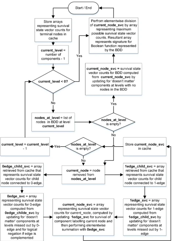
The algorithm collaborates with Reed in this part is based on the work of Reed in [66]. The state vector count or survival signature values for a system, such as a lifeline network, can be represented by a multidimensional array. The values stored at index(l1, ..., lK)of

the array stores the value corresponding tol1, ..., lK components of types 1 toKsurviving.

However, computing these arrays using enumerative methods becomes quickly infeasible since the number of state vectors to consider is equal to2m_{and therefore the computational}

complexity grows exponentially with the number of components in the network. An ef-ficient algorithm for computing the multidimensional array representation of the survival signature for a system, based on the use of the reduced ordered binary decision diagrams (BDD) data structure, is proposed.

A BDD [67] is a data structure in the form of a rooted directed acyclic graph which can be used to compactly represent and efficiently manipulate a Boolean function. It is based upon Shannon decomposition theory [68]. The Shannon decomposition of a Boolean function f on Boolean variable xi is defined as f = xi ∧fxi=1 +xi ∧fxi=0

where fxi=v is f evaluated with xi = v. Each BDD contains two terminal nodes that

represent the Boolean constant values 1 and 0, whilst each non-terminal node represents a subfunction g, is labelled with a Boolean variable v and has two outgoing edges. By applying a total ordering on them Boolean variables for functionf by mapping them to the integersx0, ..., xm−1, and applying the Shannon decomposition recursively tof, it can

be represented as a binary tree withm+ 1levels. Note that the chosen ordering can have a significant influence on the size of the BDD [69]. Each intermediate node, referred to as an if-then-else (ite) node, at levell∈ {0, ..., m−1}(where the root node is at level 0 and the nodes at levelm−1are adjacent to the terminal nodes) represents a Boolean functiong

on variablesxl, xl+1, ..., xm−1. It is labelled with variablexl and has two out edges called

1-edge and 0-edge linking to nodes labelled with variables higher in the ordering. 1-edge corresponds toxl = 1and links to the node representinggxl=1, whist 0-edge corresponds

toxl = 0and links to the node representinggxl=0. In addition, the following two reduction

rules are applied. Firstly, the isomorphic subgraphs are merged; and secondly, any node whose two children are isomorphic is eliminated.

Complement edges [70] are an extension to standard BDDs that reduce memory size and the computation time. A complement edge is an ordinary edge that is marked to

indicate that the connected child node (at a higher level) has to be interpreted as the com-plement of its Boolean function. The use of comcom-plement edges is limited to the 0-edges to ensure canonicity.

The BDD representing the system structure function for a network can be computed in various ways, e.g. from its cut-sets or network decomposition based methods [71]. In order to show the implementation of the approach, a simple network with 4 nodes and 4 edges is considered and shown in Figure 2.6.

Figure 2.6: A simple network with 4 nodes and 4 edges.

Figure 2.7: BDD for the simple network from Figure 2.6.

The corresponding BDD representing the structure function of this network, where the dashed edges represent 0-edges (marked with -1 if complemented) and solid edges repre-sent 1-edges, is shown in Figure 2.7. The survival signature from a BDD reprerepre-sentation of the system structure function for a network can then be calculated through the iterative algorithm described by Figure 2.8.

The number of operations performed during the execution of the algorithm grows ap-proximately linearly with the number of nodes in the BDD. In general, the BDD repre-sentation of the structure function for a network has far fewer nodes than2m nodes. It is therefore far more computationally efficient than using enumerative algorithms.

Figure 2.8: Algorithm for computing signature from the BDD representation of a system structure function.

2.5.3

OpenCossan

The OpenCossan engine is an invaluable tool for uncertainty quantification and manage-ment [72]. All the algorithms and methods have been coded in a Matlab toolbox allowing numerical analysis, reliability analysis, simulation, sensitivity, optimization, robust design and much more.

This thesis uses OpenCossan codes for uncertainty quantification and reliability anal-ysis on the complex systems.

Chapter 3

Complex System Reliability Analysis

Based on Survival Signature

3.1

Introduction

Most systems consist of multiple types of components in reality, contravening the iid

assumption of system signature. It would be difficult to use system signature to assess the reliability of this kind of systems, because it is hard to find rankings of order statistics of component failure times of different types. Therefore, survival signature is recognised as a better method to perform reliability analysis on complex systems and networks with multiple component types.

In this Chapter, a reliability approach based on the survival signature is proposed to analyse systems and networks with multiple types of components. The proposed approach allows us to include explicitly imprecision and vagueness in the characterisation of the uncertainties of system components. The imprecision characterises indeterminacy in the specification of the probabilistic model. That is, an entire set of plausible probabilistic models is specified using set-values (herein, interval-valued) descriptors for the descrip-tion of the probabilistic model. The cardinality of the set-valued descriptors reflects the magnitude of imprecision and, hence, the amount and quality of information that would be needed in order to specify a single probabilistic model with sufficient confidence.

In Section 3.2, the reliability assessment on systems with multiple component types is discussed. The method is based on the survival signature, which not only holds the merits of system signature, but is suitable for analysing large and complex systems and networks. Then, Section 3.3 takes uncertainty within the system into account. Both

ana-lytical methods and simulation methods are used to deal with the imprecision. After that, two survival signature-based Monte Carlo simulation methods are proposed to evaluate the system reliability in an efficient way in Section 3.4. The proposed approaches of the improved survival signature are demonstrated by some examples in Section 3.5.

3.2

Reliability Assessment on Complex System with

Mul-tiple Component Types

Now let us quantify reliability for a system with multiple component types. Assume that

Ck(t) ∈ {0,1, ..., mk}denotes the number of type kcomponents working at timet.

As-sume that the components of the same type have a known CDF,Fk(t)for typek. Moreover,

the failure times of different component types are assumed independent. Then:

P( K \ k=1 {Ck(t) =lk}) = K Y k=1 P(Ck(t) =lk) = K Y k=1 mk lk ! [Fk(t)]mk−lk[1−Fk(t)]lk (3.1)

where Ck(t) = lk means that at time t, precisely lk components of type k are working.

Hence, the survival function of the system withKtypes of components becomes:

P(Ts > t) = m1 X l1=0 ... mK X lK=0 Φ(l1, ..., lK)P( K \ k=1 {Ck(t) = lk}) = m1 X l1=0 ... mK X lK=0 Φ(l1, ..., lK) K Y k=1 mk lk ! [Fk(t)]mk−lk[1−Fk(t)]lk (3.2)

It is obvious from Equation 3.2 that the survival signature can separate the structure of the system from the failure time distribution of its components, which is the main ad-vantage of the system signature. To be specific, the survival signature part Φ(l1, ..., lK)

takes the structure of the system into consideration, which is how the state of the compo-nents influence the system performance. The part ofQK

k=1P(Ck(t) =lk)only depends on

Fk(t), which is the lifetime distribution of the components of typek.

In addition, the survival signature only needs to be calculated once for any system, which is similar to the system signature for systems with only single type of components.

It is easily seen that survival signature is closely related with system signature. For a spe-cial case of a system with only one type (K = 1) of components, the survival signature and Samaniego’s signature are directly linked to each other through Equation 2.13. How-ever, the latter cannot be easily generalised for systems with multiple types (K ≥ 2) of components.

This implies that all attractive properties of the system signature also hold for the method using the survival signature, also the survival signature is easy to apply for systems with multiple types of components, and one could argue it is much easier to interpret than the system signature. Furthermore, the difficulty of finding the probabilities of rankings of order statistics from different probability distributions can be avoided, which is indeed a simplification of computation. Finally, the quite simple survival signature (in particular for large systems with only relatively few different component types) and its monotonicity for coherent systems provides clear advantages to work towards approximations of the system reliability metrics. This does not limit the applicability of the survival signature to non-coherent systems (for example, electricity distribution network or part of the electronic equipment of safety features).

3.3

Generalised Probabilistic Description of the Failure

Times of Components

Reliability analysis of complex systems requires the probabilistic characterisation of all the possible component transitions. This usually requires a large data-set that is not always available. In fact, it might not be possible to unequivocally characterise some component transitions due to lack of data or ambiguity. To avoid the inclusion of subjective knowledge or expert opinions, the imprecision and vagueness of the data can be treated by using concepts of imprecise probabilities.

Imprecise probability combines probabilistic and set theoretical components in a uni-fied construct (see e.g. [73] [74] [75]). It allows a rational treatment of the information of possibly different forms without ignoring significant information, and without introducing unwarranted assumptions. For instance, if only few data points are available it might be difficult to identity the parameters and the form of a distribution. An unknown value of a (deterministic) parameter that is often modelled using a uniform distribution based on the principle of maximum entropy should be modelled as an interv