Credit Risk Measurement Under Basel II:
An Overview and Implementation Issues for
Developing Countries
by
CONSTANTINOS STEPHANOU & JUAN CARLOS MENDOZA
∗Abstract: The objective of this paper is to provide an overview of the changes in the calculation of minimum regulatory capital requirements for credit risk that have been drafted by the Basel Committee on Banking Supervision (Basel II). Even though the revised credit capital rules represent a dramatic change compared to Basel I, it is shown that Basel II merely seeks to codify (albeit incompletely) existing good practices in bank risk measurement. However, its effective implementation in many developing countries is hindered by fundamental weaknesses in financial infrastructure that will need to be addressed as a priority.
Keywords: Bank regulation, capital adequacy, Basel II, credit risk, developing countries
World Bank Policy Research Working Paper 3556, April 2005
The Policy Research Working Paper Series disseminates the findings of work in progress to encourage the exchange of ideas about development issues. An objective of the series is to get the findings out quickly, even if the presentations are less than fully polished. The papers carry the names of the authors and should be cited accordingly. The findings, interpretations, and conclusions expressed in this paper are entirely those of the authors. They do not necessarily represent the view of the World Bank, its Executive Directors, or the countries they represent. Policy Research Working Papers are available online at http://econ.worldbank.org.
∗ Constantinos A. Stephanou ([email protected]) is a Financial Economist in the Europe and
Central Asia Region, and Juan Carlos Mendoza ([email protected]) is a Senior Financial
Economist in the Latin America and Caribbean Region. The authors would like to exp ress their gratitude to Fernando Montes -Negret, Augusto de la Torre, Joaquin Gutierrez, Yira Mascaro and Hela Cheikhrouhou for helpful comments and suggestions. The views e xpressed in this paper are those of the authors, and do not reflect the views of the World Bank, its Executive Directors, or the countries they represent.
Public Disclosure Authorized
Public Disclosure Authorized
Public Disclosure Authorized
Public Disclosure Authorized
1. Introduction
The recent finalization of the new minimum regulatory capital requirements drafted by the Basel Committee on Banking Supervision1 (henceforth known as Basel II) has generated significant debate among academics, policy makers and industry practitioners. This interest stems both from the importance of these rules on banking systems around the world, as well as from the fact that the new rules represent a radical departure from the existing (Basel I) framework. Several different strands in the literature have recently emerged, focusing on the framework’s theoretical merits, on specific parts of the Accord (e.g. operational risk, different Pillars), on the potential impact on banking systems, and on practical implementation issues2.
This paper focuses exclusively on credit risk measurement under Basel II, and is motivated by a desire to explain the new credit capital rules (widely perceived as being overtly complex) and to discuss some practical implementation problems for developing countries. In particular, the objectives of this paper are threefold:
• to describe some of the theoretical and empirical developments in credit risk measurement that have motivated and shaped the new rules
• to summarize the treatment of credit risk (particularly under Pillar 1) in Basel II
• to identify implementation issues and some policy implications for developing countries.
The paper concludes that although the revised credit capital adequacy rules represent a dramatic change compared to the Basel I framework, Basel II merely seeks to codify (albeit incompletely) existing good practices in bank risk measurement. However, its effective implementation in many developing countries is hindered by fundamental weaknesses in financial infrastructure that will need to be addressed as a priority.
The rest of this section contains a brief overview of the Basel I and II frameworks. Section 2 describes the key building blocks for measuring credit risk. Section 3 summarizes the new credit capital rules of Basel II, and Section 4 discusses practical implementation problems for developing countries and draws relevant policy implications.
1
The Basel Committee on Banking Supervision is a committee comprising of senior bank supervisory authority and central bank representatives from the G-10 countries. The Committee does not possess any formal supranational supervisory authority, but it formulates (by consensus) broad supervisory standards and promotes best practices in the expectation that each country will implement them in ways most appropriate to its circumstances.
2
The bibliography at the end of this paper contains some of the most important recent contributions to the literature, while reference to specific publications (where appropriate) is made throughout the text.
Basel I
The Basel I Capital Accord, published in 19883, represented a major breakthrough in the international convergence of supervisory regulations concerning capital adequacy. Its main objectives were to promote the soundness and stability of the international banking system and to ensure a level playing field for internationally active banks. This would be achieved by the imposition of minimum capital requirements for credit (including country transfer) risk, although individual supervisory authorities had discretion to build in other types of risk or apply stricter standards. Even though it was originally intended solely for internationally active banks in G-10 countries, it was eventually recognized as a global standard and adopted by over 120 countries around the world.
The framework defined the constituents of ‘regulatory capital’ (numerator of the solvency formula) and set the risk weights for different categories of on- and off-balance sheet exposures (denominator of the solvency formula). The risk weights, which were intentionally kept to a minimum (only five categories/buckets), reflected relative credit riskiness across different types of exposures. The minimum ratio of regulatory capital to total risk-weighted assets (RWA) was set at 8%, of which the ‘core capital’ element (a more restrictive definition of eligible capital known as Tier 1 capital) would be at least 4%. The most important amendment to the framework took place in 1996, when an additional capital charge was introduced to cover market risk in banks’ trading books4. However, the basic credit risk capital measurement framework remained unchanged, although the definition of assets and capital has evolved over the years in response to financial innovation.
Although the Basel I framework helped to ‘level the playing field’ and to stabilize the declining trend in banks’ solvency ratios, it suffered from several problems that became increasingly evident over time:
• Lack of sufficient risk differentiation for individual loans. The weights did not sufficiently differentiate credit risk by counterparty (i.e. financial strength) or loan (e.g. pledged collateral, covenants, maturity) characteristics. For example, the capital charge for all corporate exposures was the same irrespective of the borrower’s actual rating. This implied that banks with the same capital adequacy ratio (CAR) could have very different risk profiles and degrees of risk exposure.
• No recognition of diversification benefits. Standard portfolio theory recognizes the risk reduction benefits attained from diversification. However, because Basel I was based on the ‘building blocks’ approach, there was no distinction or difference in capital treatment between a well-diversified (less risky) loan portfolio from one that is very concentrated (and hence riskier).
• Inappropriate treatment of sovereign risk. Basel I’s capital treatment for sovereign exposures made little economic sense, and the mechanical application of these rules often created perverse incentives and led to the mispricing of risks. For example, lending to OECD governments became more attractive because it incurred no regulatory capital charge, even though this group included countries
3
See Basel Committee on Banking Supervision (July 1988). 4
with substantially different credit ratings such as Turkey, Mexico and South Korea. Claims to the national central government also enjoyed a zero risk weight, encouraging many banks (particularly in developing countries) to ignore basic diversification principles and lend heavily to their sovereigns (directly or through state-owned enterprises), thereby reducing financial intermediation.
• Few incentives for better overall risk measurement and management. The lack of emphasis on other risk types (e.g. interest rate, operational, business) and on financial infrastructure issues (e.g. accounting, legal framework) did not provide adequate incentives to encourage complementary improvements in banks’ risk governance and measurement. As a result, there was often an excessive reliance on, and a false comfort from, a high capital adequacy ratio. Subsequent experience has shown that such a ratio, by itself, is meaningless in the absence of other supporting measures.
The shortcomings of Basel I5 meant that regulatory capital ratios were increasingly becoming less meaningful as measures of true capital adequacy, particularly for larger, more complex institutions. In addition, various types of products (e.g. 364-day revolvers and ‘balance sheet’ securitizations) were developed primarily as a form of regulatory capital arbitrage to overcome those rules. Finally, the state of risk measurement and management evolved significantly in the last 15 years, allowing many banks to develop their own sophisticated internal economic capital models (oftentimes running parallel to regulatory capital ones) to guide business decisions. The relegation of regulatory capital measurement and reporting to primarily a compliance and public relations6 exercise also had the perverse effect of distancing bank supervisors from the actual risk assessment process and the manner in which those banks were run, since Basel I ratios in many cases formed the sole legal basis for taking supervisory action.
Overview of Basel II
Following the publication of successive rounds of proposals between 1999 and 2003, active and broad consultations with all interested parties, and related quantitative impact studies, the Basel Committee members agreed in mid-2004 on a revised capital adequacy framework (Basel II)7. The framework will be implemented in most G-10 countries as of year-end 2006, although its most advanced approaches will require one further year of impact studies or “parallel running” and will therefore be available for implementation one year later8. For banks adopting the IRB approach for credit risk or the AMA for operational risk, there will be a capital floor following implementation of the framework as an interim prudential arrangement.
5 The Basel Core Principles (BCPs) for effective supervision seek to address some of these shortcomings by, for example, calling for capital requirements for interes rate and market risks. However, they lack any explicit regulatory guidelines.
6
This does not mean that the actual regulatory CAR has become unimportant for bank management, regulators, rating agencies and investors, but that it provides (at least for sophisticated banks) little guidance as to the true riskiness of the business, or to the way that it is run.
7
See Basel Committee on Banking Supervision (June 2004). 8
Some countries (e.g. Australia) have publicly expressed their intention to adopt a single end-2007 start date instead of a ‘staggered’ one.
The main objective of the framework is to further strengthen the soundness and stability of the international banking system via better risk management, by bringing regulatory capital requirements more in line with (and thus codifying) current bank good practices. This will be achieved by making credit capital requirements significantly more risk-sensitive and by introducing an operational risk capital charge. The intention is to broadly maintain the aggregate level of capital requirements9, but provide incentives to adopt the more advanced risk-sensitive approaches of the revised framework. These changes are implemented by changing the definition of Risk Weighted Assets (i.e., the denominator of the CAR) while leaving most of the other elements of Basel I unchanged, such as the focus on accounting data, the definition of eligible capital, the 8% minimum CAR requirement and the 1996 market risk amendment to the Capital Accord.
Basel II consists of a broad set of supervisory standards to improve risk management practices, which are structured along three mutually reinforcing elements or pillars:
• Pillar 1, which addresses minimum requirements for credit and operational risks
• Pillar 2, which provides guidance on the supervisory oversight process
• Pillar 3, which requires banks to publicly disclose key information on their risk profile and capitalization as a means of encouraging market discipline.
Compared to Basel I, the scope of application is broader and includes, on a fully consolidated basis, all major internationally active banks at every tier within a banking group (i.e. full sub-consolidation), as well as at the level of the group’s holding company10. Supervisors also need to ensure that individual banks within the group remain adequately capitalized on a stand-alone basis. Consolidation must capture, to the greatest extent possible, all banking and relevant financial activities (both regulated and unregulated) with the exception of insurance. Significant minority investments where control does not exist, as determined by national accounting and/or regulatory practices, will either be deducted from equity or consolidated on a pro-rata basis. However, significant minority and majority investments in commercial entities that exceed certain materiality levels (subject to some national discretion) will be deducted from banks’ capital.
Before describing Basel II in greater detail, it is necessary to briefly review the credit risk concepts that have been developed by leading financial institutions in the last 10-15 years and that constitute the basis of the Accord’s credit risk measurement framework.
9
In fact, the Committee declared its willingness to review the calibration of the framework prior to implementation and apply a scaling factor to ensure that aggregate minimum capital requirements are broadly maintained.
10
This is the minimum requirement for G-10 countries. Some of these (e.g. EU members) have gone beyond this minimum and intend to extend the application of Basel II to all domestic banks and investment firms.
2. Credit Risk Building Blocks
Credit risk has been traditionally defined as default risk, i.e. the risk of loss from a borrower/counterparty’s failure to repay the amount owed (principal or interest) to the bank on a timely manner based on a previously agreed payment schedule. A more comprehensive definition would actually include value risk, i.e. the risk of loss of value from a borrower migrating to a lower credit rating (opportunity cost of not pricing the loan correctly for its new level of risk) without having defaulted. In order to protect themselves against volatility in the level of default/value losses (as well as other types of risk), banks have adopted methodologies that allow them to quantify such risks and thereby derive the amount of capital required to support their business – what is referred to as economic capital. The building blocks of economic capital for default-related credit risk are discussed below11.
It should be noted that the calculation of economic capital takes a purely ‘economic’ view of the business, which often differs from the one represented by financial statements. For example, when there is a credit deterioration of the borrower, the resulting value loss is often not shown (at least immediately) in the bank’s balance sheet and income statements. This is because many credit exposures are recorded on an accrual basis as opposed to market/fair value, meaning that a loss in the value of a downgraded loan is not realized until the loan actually defaults or is sold to a third party at arm’s length. As a result, economic capital models that feed into risk adjusted return on capital (RAROC) performance measures12 often paint a different, more realistic and dynamic picture of a bank’s profitability than what is shown in traditional financial statements.
Expected Versus Unexpected Loss
Although credit losses naturally fluctuate over time and with economic conditions, there is (ceteris paribus) a statistically measured, long-run average loss level. Assume for example that, based on historical performance, a bank has come to expect around 1% of its loans to default every year, with an average recovery rate of 50%. In that case, the bank’s expected loss (EL) for a credit portfolio of $1 billion is $5 million (i.e. $1 billion x 1% x 50%). As can be deduced, EL is based on three parameters:
• The likelihood that default will take place over a specified time horizon (probability of default or PD)
• The amount owned by the counterparty at the moment of default (exposure at default or EAD)
• The fraction of the exposure, net of any recoveries, which will be lost following a default event (loss given default or LGD).
11
The rest of the section discusses default risk, which is the main focus of Basel II’s Pillar 1. Value risk, which necessitates a substantial modeling exercise to value each credit exposure in each possible migratory state and then probability-weigh them to arrive at the expected change in the credit’s value, is not covered. 12
RAROC sought to replace the traditional ROE (Return on Equity) measure by explicitly tying returns to true economic risk. This was to be achieved by incorporating the cost of such risk in the returns (i.e. the numerator of the equation) and dividing the result by economic capital (as opposed to book capital).
Since PD is normally specified on a one-year basis13, the product of these three factors is the one-year EL as follows:
EL = PD x EAD x LGD
EL can be aggregated at various different levels (e.g. individual loan or entire credit portfolio), although it is typically calculated at the transaction level; it is normally mentioned either as an absolute amount or as a percentage of transaction size. It is also both customer- and facility-specific, since two different loans to the same customer can have a very different EL due to differences in EAD and/or LGD.
It is important to note that EL (or, for that matter, credit quality) does not by itself constitute risk; if losses always equalled their expected levels, then there would be no uncertainty. Instead, EL should be viewed as an anticipated “cost of doing business” and should therefore be incorporated in loan pricing and ex ante provisioning.
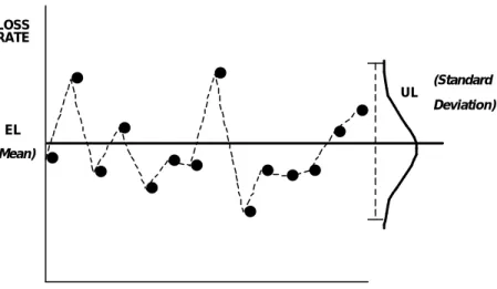
Credit risk, in fact, arises from variations in the actual loss levels, which give rise to the so-called unexpected loss (UL). Statistically speaking, UL is simply the standard deviation of EL (see Figure 1). As will be described later, the need for bank capital stems from the desire to cushion against loss volatility (UL) at a certain confidence level.
Figure 1: Expected and Unexpected Loss
•
•
•
•
•
•
•
•
•
•
•
•
•
•
UL EL LOSS RATE (Mean) (Standard Deviation) TIME Probability of Default (PD)Financial institutions have traditionally attempted to minimize the incidence of credit risk primarily via a loan-by- loan analysis carried out during the credit underwriting process. The foundations of a more analytical framework began in the early 1960s when the first
13
Although the one-year horizon is fairly arbitrary, it is reasonable from a bank management perspective because it coincides with the typical budgeting period and because it can be considered a reasonable timeframe within which to raise new share capital to cover additional losses that might have occurred.
“credit scoring” models were built to assist credit decisions for consumer loans14. Although they initially classified debtors/counterparties on default potential based only on an ordinal ranking, they were the original precursors to numerical PD estimation. By the mid-1980s, particularly with the introduction of RAROC as a performance measure, leading financial institutions began calibrating each credit score to a particular PD15 to estimate EL and ultimately economic capital.
The measurement of a PD pre-supposes the use of a definition of default that has tended to vary across credit institutions16, thereby hindering comparisons. The definitions have started to converge in recent years, while Basel II adopts a reference default definition to facilitate comparability of capital results.
Several techniques have subsequently been developed to calculate PD, which can be divided into two broad categories: empirical and market-based (also known as structural or reduced-form) models. The former use historical default rates associated with each score to identify the characteristics of defaulting counterparties, while the latter use counterparty market data (e.g. bond or credit default swap spreads, volatility of equity market value) to infer the likelihood of default.
The empirical approach uses historical default data to characterize counterparties that default. This was originally done using discriminant analysis (Z scores) but more recently has been done with logit or probit regressions to define a score function S of the form:
1 1 2 2
( )i ... n n
S x =β x +β x + β x
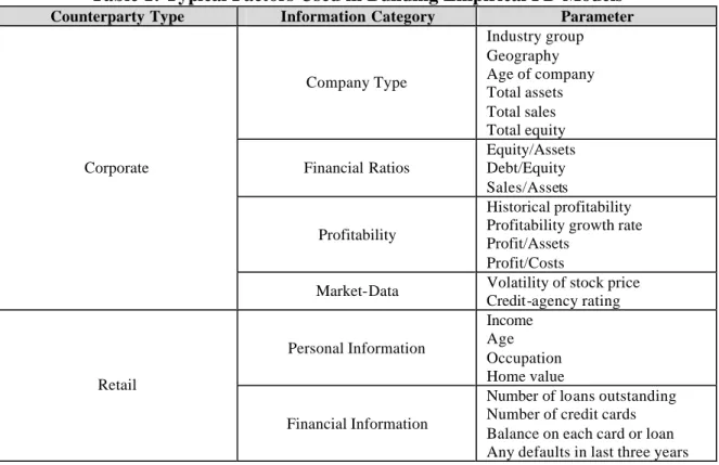
The vector x contains the relevant risk factors, which in the case of commercial counterparties may be primarily financial statement ratios and non- financial information (e.g. management quality, years in operation); for retail customers, this might include income, work history and other demographic data17. Table 1 presents a set of illustrative factors typically used in these models18.
14
This was driven by the recognition that expensive judgment-based analysis carried out for commercial loans was simply not cost-effective for mass-market retail (and eventually small business) exposures. 15 Until Basel II formalized the use of PD, this concept was often called Expected Default Frequency. 16 The non-payment past due ‘threshold’ period triggering a default event h as historically ranged from a day to a few months or even years, depending on the instrument, jurisdiction and (where it is not mandated by legal or supervisory norms) the bank involved.
17
Different jurisdictions regulate differently the kind of demographic data that can be used to make lending decisions to avoid discrimination on the basis of, for example, gender or race.
18
There is no clear standard on what the appropriate predictive power of a model should be. Comparisons between models are normally carried out by drawing power curves, i.e. by sorting the customers according to their scores on the horizontal axis and generating a graph with the percentage of all the defaults in the sample covered by those customers on the vertical axis. Reasonable models should generally capture about 90% of defaults in a year from around 20% of the lower-rated scores (Kealhofer, 2003).
Table 1: Typical Factors Used in Building Empirical PD Models
Counterparty Type Information Category Parameter
Company Type Industry group Geography Age of company Total assets Total sales Total equity Financial Ratios Equity/Assets Debt/Equity Sales/Assets Profitability Historical profitability Profitability growth rate Profit/Assets
Profit/Costs Corporate
Market-Data Volatility of stock price Credit-agency rating Personal Information Income Age Occupation Home value Retail Financial Information
Number of loans outstanding Number of credit cards Balance on each card or loan Any defaults in last three years
Adapted from Marrison (2002).
The statistical model generates an ordinal score that ranks counterparties according to their likelihood of default, or it can directly provide an unadjusted PD19. In both cases, the results of the model need to be calibrated to obtain a cycle-neutral cardinal scale. This can be done in several different ways depending on how much historical data is available. For example, the cycle neutral central tendency of the entire portfolio can be identified and used as an anchor point to adjust the PDs calculated with data from a limited part of the economic cycle.
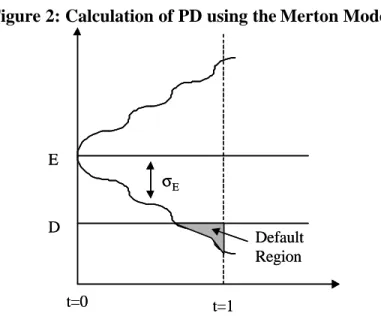
By contrast, the market-based approaches use current market data about debt and/or equity to “back out” a market-driven measure of PD. This method was developed by Merton (1974) and popularized by the company KMV (now owned by Moody’s). Merton modeled the holding of a company’s debt as being equivalent to holding debt of a risk-free company plus being short a put option on the assets of the company: if the value of the assets falls below the value of the debt, the shareholders can put the company’s assets to the debt holders and avoid repaying the debt, given that they are normally covered by limited liability arrangements.
The PD can be easily derived from equity prices if one assumes that market capitalization is a good proxy for the value of the firm’s assets and that asset values (E) are normally distributed. On this basis, a distance to default (DD) concept can be defined as:
19
Since both point-in-time and historical information is included, the PD is unadjusted in the sense that the data may not appropriately cover an entire economic cycle. An adjusted PD represents an economic cycle -neutral estimate which can be conceptualized as the average PD during the entire cycle.
E E D DD σ − =
where D is the expected future level of debt and σE is the observed volatility of asset prices. If E drops below D, the company would default and, assuming that the company’s value is normally distributed, the PD is equal to the area under the curve (see Figure 2).
Figure 2: Calculation of PD using the Merton Model
E D t=0 t=1 Default Region σE E D t=0 t=1 Default Region σE
Adapted from Saunders (1999)
Similar models exist that use bond or credit default swap prices to derive a PD assuming ‘risk neutral’ pricing, i.e. whereby the value of a risky bond (its face value discounted at its risk-adjusted discount rate) is equal to its expected value in the future discounted at the risk- free rate. However, “backing-out” the PD from bond spreads has several problems, such as the fact that the spreads also include an implied LGD figure, implying that PD can only be uniquely determined if we already know LGD.
The main disadvantages of market-based methods are the following:
• they can only be used for publicly traded borrowers in well- functioning markets
• they tend to be ‘black boxes’ whose outcomes can often lack intuition
• they often lead to highly volatile levels of PD and capital.
On the other hand, the continuous market information updates (when they exist) often make these methods more reliable than those based on historical accounting data, which are only updated periodically or with a lag20. As a result, the two methodologies tend to co-exist within sophisticated banks and be primarily used for different types of credit exposures. However, in the case of non-corporate loans and for banks in most emerging economies, the empirical method is often the only realistic option.
20
For example, one can compare the (slow) adjustment of Enron’s official credit ratings prior to default with those that were provided by market-based models.
Exposure at Default (EAD)
EAD refers to the outstanding amount at the time of default. In the simple case of a loan, the exposure is assumed to be fixed for each year and can be derived from the agreed amortization plan. In the case of derivatives, it requires more complex simulations to estimate the path that the underlying value of the asset may take and thus the potential future exposure that would arise21.
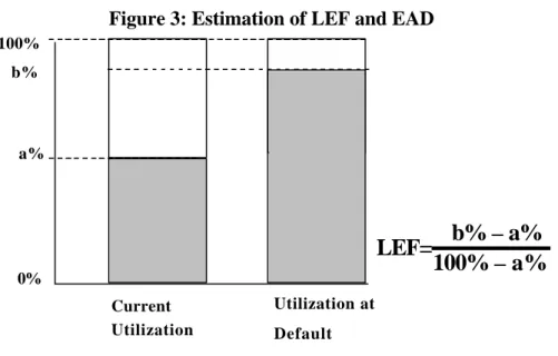
In the case of lines of credits or any other type of revolving facility, EAD is generally estimated using empirical data by looking at the distribution of utilization levels of credit lines prior to the moment of default, as expressed in the following equation:
ExposureatDefault=CurrentExposure+LEF×UnutilisedPortionof theLimit
LEF is the Loan Equivalency Factor and represents the portion of the unutilized line that is expected to be drawn down before default (see Figure 3). Generally, a “race to default” takes place whereby lines are quickly drawn down shortly before default. Most empirical studies indicate that the counterparty’s facility type and pre-default credit grade are good LEF predictors. Counterparties that default despite having a good credit rating generally default due to an unforeseen ‘disaster’ (e.g. fraud) and have less time to draw down credit lines, as opposed to counterparties that have been slowly downgraded and will increasingly utilize their credit lines.
Figure 3: Estimation of LEF and EAD
100% a% 0% Current Utilization Utilization at Default
LEF=
b%b% – a%
100% – a%
21The current mark-to-market (MTM) value of a derivative is effectively a probability weighted average of all future possible values, both negative and positive. By contrast, Potential Future Exposure for credit risk calculations is the probability weighted average of only future positive MTM values, replacing all future negative MTM values by zero. This leads to a truncation of the probability distribution of future MTM values, which shifts its mean to the right.
Loss Given Default (LGD)
LGD is the percentage of the EAD that is lost in the event of a default22. Its calculation requires answering the following questions:
• How much is recovered and from where (e.g. collateral liquidation)?
• How long did it take to recover and what is the financial cost (i.e. interest income forgone) associated with this period of time?
• How much had to be spent in the recovery process (i.e. workout expenses)? There are three main types of LGD measurement23. The first one (workout LGD) is based on the estimation and timing of cash flows and costs from the workout process:
EAD Recovery Admin
LGD
EAD
− +
=
For the estimation to be accurate, all figures must be expressed in present value terms to take into account time effects since the recovery process can be very long. Recovery refers to the present value of the total recovered amount and is a function of the country (legal regime, court efficiency and insolvency proceedings), loan seniority, industry and collateral presence (type, amount etc.). Admin includes all the related workout costs that were incurred (e.g. legal and collection fees). Workout LGD is by far the most common approach in the case of most loan types, particularly for a bank that has sufficient historical loss experience with these variables. The level of sophistication in its LGD calculation varies from a single look- up table with a few values to an advanced econometric model or neural network with several causal variables.
The second type of LGD measurement (market LGD) can be observed from market prices and trades of defaulted bonds or loans after the actual default event. In the exceptional case that a liquid distressed debt market exists, LGD can be written as:
ValueBefore ValueAfter LGD
ValueBefore − =
where Value refers to the valuation before and after (i.e. sale price, reflecting the market’s expected present value of eventual recovery) the time of default. Because these transactions take place at arm’s length, they are less subject to potential valuation problems. Most rating agency recovery studies are based on this approach.
Finally, the third type of LGD measurement (implied market LGD) is derived from the prices of fixed income and credit derivatives products using a theoretical asset-pricing model. This approach essentially ‘backs out’ LGD from the credit spreads of risky (but not defaulted) bonds or from credit default swap prices, but it is limited in scope (traded
22
Until Basel II formalized the use of LGD, this concept was also called Severity. 23
debt only) and subject to methodological problems (credit spread also reflects PD and potentially a liquidity premium, tax considerations etc.).
Unexpected Loss (UL) for a Single Loan
UL is simply the volatility in the components of EL that were described above:
( ) ( )
UL=σ EL =σ PD EAD LGD× ×
In order to solve this equation, it would be necessary to know the standard deviation of all three variables. In the case of PD, since it reflects an underlying Bernoulli variable (i.e. a variable than can only have two states – the counterparty defaults or not), its standard deviation is equal to:
(PD) PD(1 PD)
σ = −
Some practitioners also assume that the variance of EAD and LGD is zero24. As a result, the UL equation for a single loan (what is often referred to as the ‘stand-alone UL’) is often simplified as follows:
( )
UL= EL EAD LGD EL× −
Portfolio- and Bank-Level UL
The most important point of departure between traditional bottom up (i.e. loan-by- loan) and modern credit analysis is the treatment of portfolio- level effects that derive from correlations (both within and across portfolios). Unlike EL, the bank- or portfolio- level UL is not equal to the sum of individual ULs; that is because variance is not an additive parameter, but depends critically on the loss correlations between all the loans in the portfolio. A highly correlated portfolio implies a more skewed loss distribution and would require, ceteris paribus, a higher level of capital than a more diversified portfolio25. That has a major implication for credit risk management: an individual loan’s marginal contribution to portfolio credit risk (referred to as the loan’s ‘contributory UL’ to distinguish it from ‘stand-alone UL’) critically depends on the properties of the portfolio in which it is held.
The EL for a portfolio p with N loans is simply the sum of the EL for each loan:
1 N P i i EL EL = =
∑
24In the case of EAD, the justification for this assumption is that we are referring t o a normal term loan whose EAD is fixed at 1. In the case of LGD, however, the assumption does not hold well because LGD has often empirically exhibited a binomial distribution and has tended to vary over the business cycle. 25
In intuitive terms, a highly correlated portfolio contains loans that tend to default together more often, thereby exacerbating credit losses experienced during bad times. Such a portfolio would exhibit a loss distribution with a much longer tail implying that, for the same EL, its UL would be much greater.
However, the portfolio UL must exp licitly take account of intra-portfolio correlations: 2 , 1 1 N N P i j i j i j UL ρ ULUL = = =
∑∑
where ρi,j is the pair-wise correlation between loans i and j. A correlation of 1 would
imply that when one defaults the other one does too simultaneously. A correlation of 0 means that they tend to default completely independently of each other. For practical purposes, loss correlation is often simplified to default correlation, which is used to measure the extent to which counterparties tend to default simultaneously.
The methods of analysis used to calculate these correlations are beyond the scope of this document, but a common simplifying assumption is to define a single ρ for a portfolio with a specific country, industry and/or rating profile (e.g. US investment grade telecom exposures). This default correlation can be calculated in a credit portfolio model by observing asset correlation movements (i.e. stock prices) of relevant public companies, or through direct observation of historical data, a method more amenable to retail portfolios that have large default datasets. Making this assumption, the ULP simplifies to:
1 N P i i UL ρ UL = =
∑
Since a typical bank contains several credit portfolios (each with a different ρ), deriving the bank-wide UL is a complex calculation consisting of the individual ULP and a
correlation matrix between the different portfolios (i.e. inter-portfolio correlations). The above discussion has used a frequent, albeit incorrect, simplifying assumption that all portfolios are infinitely granular, i.e. no single portfolio exposure accounts for more than an arbitrarily small share of the total. In reality, many portfolios tend to be ‘lumpy’ (i.e. made up of fewer relatively large loans), which implies that idiosyncratic risk is not diversified away completely and that capital estimates based only on systematic risk factors are understated. In that situation, an add-on granularity factor needs to be added to the correlations that give rise to portfolio- level diversification effects.
Portfolio Loss Distribution and Economic Capital
The aforementioned building blocks allow the estimation of the mean (EL) and variance (UL) of credit losses, but the shape of the entire portfolio- level loss distribution is still not known. There are two main ways of deriving it: the closed- form and the simulation/value-at-risk approach. The former simply imposes a specific distributional assumption (e.g. beta distribution) to replicate what has been observed empirically, while the latter uses a Monte Carlo simulation to explicitly construct a portfolio loss distribution. Numerous commercial credit value-at-risk models have been developed in the last 10-15 years (e.g. CreditMetrics, KMV, CreditRisk+) that use the main credit risk inputs described above to derive a loss distribution, by assuming that correlations across borrowers arise due to common dependence on a set of ‘systematic risk factors’ (essentially variables representing the state of the economy). Sophisticated banks typically use these models nowadays for active portfolio- level credit management
(particularly for large corporate loans) by identifying risk concentrations and opportunities for diversification via debt instruments and credit derivatives.
Once the bank- level credit loss distribution is constructed, credit economic capital is simply determined by the bank’s tolerance for credit risk, i.e. the bank needs to decide how much capital it wants to hold in order to avoid insolvency because of unexpected credit losses over the next year. A safer bank must have sufficient capital to withstand losses that are larger and more rare, i.e. they extend further out in the loss distribution tail. In practice, therefore, the choice of confidence interval in the loss distribution corresponds to the bank’s target credit rating (and related default probability) for its own debt. For example, a bank that wants its public debt to be rated AA needs (based on historical default rates of AA rated companies) to hold enough capital to have a 99.97% survival probability over a one- year time horizon. As Figure 4 shows, economic capital is the difference between EL and the selected confidence interval at the tail of the loss distribution; it is equal to a multiple K (often referred to as the capital multiplier) of the standard deviation of EL (i.e. UL).
Figure 4: Credit Economic Capital and the Loss Distribution
The shape of the loss distribution can vary considerably depending on product type and borrower credit quality. For example, high quality (low PD) borrowers tend to have proportionally less EL per unit of capital charged, meaning that K is higher and the shape of their loss distribution is more skewed (and vice versa).
The loss distribution and associated economic capital can be calculated at various levels within the organization, although the desired confidence interval (level of protection) must be applied consistently. At a bank-wide level, the capital adequacy of the institution (once credit capital is combined with capital for other risk types) can be evaluated by
comparing required economic capital with available financial resources. At a business unit level, capital consumption can be used as an input in the unit’s RAROC or Shareholder Value Added (SVA)26 calculations. At a transaction level, it can be used to correctly price the risk undertaken. It is worth noting that different assumptions about diversification benefits need to be made at each of these levels. For example, when capital is calculated for a business unit or a transaction, it can be on a stand-alone basis or on a contributorybasis. In the first case, the business unit or the transaction is seen as disconnected from the rest of the bank and does not therefore gain any of the diversification benefits that come as a result of being part of a bigger institution27. In the second case, credit risk correlations with the rest of the bank exposures (and therefore additional diversification benefits) are taken into account.
EL and Economic Capital Versus Provisions and Regulatory Capital
EL and economic capital for credit risk are conceptually (if not explicitly) comparable to loan loss provisions and regulatory capital. Although the latter two variables also attempt to estimate the amount of expected and unexpected credit losses respectively, their methodologies are much cruder and fraught with problems. In particular, loan loss provisions are primarily based on a combination of country-specific regulatory, tax and accounting considerations; these drive a wedge between statistically driven EL and actual provisions, since the latter are generally based on the concept of incurred losses28. By comparison, EL and economic capital come from different parts of the same loss distribution and are therefore consistent with each other. As will be seen in the next section, Basel II aligns regulatory capital for credit risk much closer to economic capital, which also has implications for the relation between EL and loan loss provisions.
26 An SVA or EVA (Economic Value Added) framework attempts to measure the economic value added/profit of a business line (or of the entire bank) by using a target hurdle rate to adjust the accounting profit so that it includes the o pportunity cost of the economic capital that is needed to support that business. 27
In intuitive terms, the credit capital of a loan to a US corporate would not include the diversification benefits of (lower correlated) loans to UK mortgages, even though the bank might be active in both business lines. Particularly when RAROC is used to measure the performance of individual business units, economic capital is typically calculated without such diversification benefits.
28
This inconsistency of treatment is currently being discussed between the Basel Committee and the International Accounting Standards Board (IASB).
3. Credit Risk Framework under Basel II29
In contrast to Basel I that applies a “one size fits all” approach to all banks, Basel II offers a menu of options under Pillar 1 for calculating the credit capital requirements of banking book exposures30. In particular, two main methodologies can be used for most exposures: the Standardized Approach and the Internal Ratings Based (IRB) Approach; securitization exposures are subject to a separate (but similar) capital treatment. Each approach has different characteristics and requirements that are briefly described below.
Standardized Approach
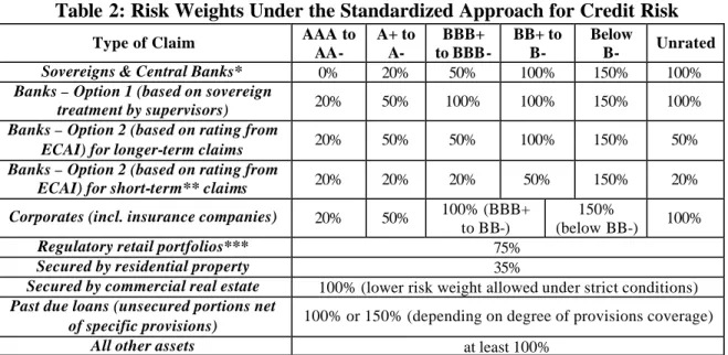
This approach measures credit risk similar to Basel I, but has greater risk sensitivity because it uses the credit ratings of external credit assessment institutions (ECAIs) to define the weights used when calculating RWAs. National supervisors are responsible for recognizing ECAIs in accordance with specific eligibility criteria (e.g. objectivity, independence, disclosure of methodologies etc.) mentioned in the document, as well as for mapping their assessments to the risk weights available.
Table 2: Risk Weights Under the Standardized Approach for Credit Risk
Type of Claim AAA to
AA- A+ to A- BBB+ to BBB- BB+ to B- Below B- Unrated Sovereigns & Central Banks* 0% 20% 50% 100% 150% 100%
Banks – Option 1 (based on sovereign
treatment by supervisors) 20% 50% 100% 100% 150% 100% Banks – Option 2 (based on rating from
ECAI) for longer-term claims 20% 50% 50% 100% 150% 50% Banks – Option 2 (based on rating from
ECAI) for short-term** claims 20% 20% 20% 50% 150% 20% Corporates (incl. insurance companies) 20% 50% 100% (BBB+
to BB-)
150%
(below BB-) 100%
Regulatory retail portfolios*** 75%
Secured by residential property 35%
Secured by commercial real estate 100% (lower risk weight allowed under strict conditions)
Past due loans (unsecured portions net
of specific provisions) 100% or 150% (depending on degree of provisions coverage)
All other assets at least 100%
Source: Basel Committee on Banking Supervision (June 2004).
Note 1: Claims to non-central government public sector entities can be treated either as claims on banks or the relevant sovereign Note 2: Off-Balance Sheet items will be converted to credit exposure equivalents using credit conversion factors
* As an alternative to ECAI ratings, the country risk scores assigned by Export Credit Agencies (ECAs) recognized by national supervisors, or the consensus risk scores published by the OECD in the “Arrangements on Guidelines for Officially Supported External Credits”, may be used. To qualify, an ECA must publish its risk scores and subscribe to the OECD-agreed methodology. ** Short-term claims must have an original maturity of three months or less.
*** In order to qualify, claims must meet criteria relating to orientation, product, granularity and low value of individual exposures.
29
See Basel Committee of Banking Supervision (June 2004) for a comprehensive and detailed description of the framework.
30
There is also a counterparty credit risk capital charge for over-the-counter derivatives, repo-style and other transactions booked in the trading book, separate from the capital charge for general market risk and specific risk. The risk weights to be used must be consistent with those used for calculating the capital requirements in the banking book (i.e. Standardized or IRB Approaches).
Table 2 illustrates the risk weights by type of counterparty and credit rating. However, considerable national discretion exists – for example, supervisors may:
• select a lower risk weight to apply to banks’ exposures to their sovereign (and by implication to other domestic banks under Option 1 below) as long as the exposure is in domestic currency and funded in that currency
• permit banks to risk weight all corporate claims at 100% irrespective of the existence of external ratings
• apply higher risk weights for regulatory retail, unrated corporate claims etc. Credit risk mitigants are recognized for regulatory capital purposes as long as:
• General requirements for legal certainty are satisfied (e.g. the enforceability of master netting agreements)
• Mitigants are not double counted (i.e. not already reflected in an issue-specific rating used to determine risk weights)
• Remaining residual risks are properly accounted for
• Minimum conditions relating to collateral treatment are observed.
Banks may opt either for the simple approach (i.e. substitute risk weight of collateral for the risk weighting of the counterparty), or for the comprehensive approach (i.e. estimate volatility-adjusted amounts for both exposure and collateral) to credit risk mitigation. Although the latter approach recognizes more collateral instruments as eligible mitigants, it also imposes supplementary criteria depending on whether banks use standard supervisory haircuts or their own estimates/VAR models to calculate market price and foreign exchange volatility. Additional operational requirements are also necessary for the recognition of guarantees and credit derivatives as risk mitigants.
In order to provide additional guidance for smaller systems/less sophisticated supervisors, the Basel Committee has collected the simplest available options for calculating risk-weighted assets (including securitization exposures) under a so-called “Simplified Standardized Approach”. It is expected that bank supervisors from many developing countries will (at least initially) adopt this simpler version of the Standardized Approach.
IRB Approach
The IRB Approach is a more sophisticated methodology, since it is primarily based upon the credit risk building blocks described in the previous section. Subject to certain minimum conditions and disclosure requirements, this approach relies on banks’ own internal estimates of certain risk parameters to determine credit capital requirements. However, the capital figure itself is still derived from a supervisory formula provided by the Basel Committee that has been calibrated to reflect the risk of specific asset types and to ensure that overall capital levels in G-10 countries remain broadly unchanged.
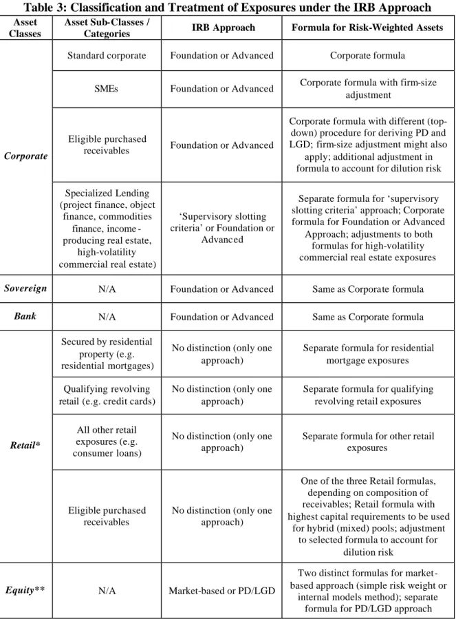
Under the IRB Approach, all banking book exposures must be categorized into broad asset classes using specific definitions and criteria provided by the Committee. For each of these asset classes, there are distinct:
• Risk components – estimates of risk parameters (PD, LGD, EAD, effective maturity) that can be calculated by banks themselves or provided by supervisors
• Risk-weight functions – the formulas by which risk components are transformed into risk-weighted assets and therefore capital requirements
• Minimum requirements – minimum standards for a bank to use the IRB approach for a given asset class.
For corporate, sovereign and bank exposures, the RWAs are calculated as follows:
50 50 50 50 1 1 Correlation ( ) = 0.12 0.24 1 1 1 PD PD e e e e ρ × − − ×− + × − − − ×− − −
(
)
2 Maturity Adjustment ( ) = 0.11852 0.05478 ln(b − × PD)Risk-weighted assets (RWA) = 12.5K× ×EAD
Capital charge = 8%×RWA
where:
Φ-1
(z) is the inverse cumulative distribution function (c.d.f.) for a standard normal random variable, i.e. the value of y such that Φ (y) = z
Φ(y) is the c.d.f. for a standard normal random variable ln(PD) is the natural logarithm of the PD
M is effective (remaining) maturity
Although the capital formula appears rather daunting and unintuitive31, it is worth highlighting some of its main characteristics:
• A loss correlation is included but modeled solely as a function of PD, thereby ignoring (or at least moving to Pillar II) potentially important portfolio characteristics such as industry and geographic diversification32
31 See Wilde (May 2001) and Gordy (October 2002) for a technical, and Fitch Ratings (August 2004) for a non-technical, description of the formula. Formally speaking, the formula is based on a one-factor model, meaning that there is only one systematic factor (as a proxy for general economic conditions) that drives correlations across borrowers. This is important because (together with the infinite granularity assumption) it gives rise to additive, portfolio-invariant contributions to capital, i.e. the IRB capital requirements only depend on each individual loan’s own characteristics and do not have to be calibrated for each portfolio based on its particular composition.
32
Formulas for other asset classes differ in their approach to these parameters, but a common characteristic is that lower quality (higher PD) assets have lower correlations. This corresponds to the empirical finding that lower quality exposures are driven mainly by idiosyncratic (borrower-specific) factors and thus relatively less by broader market events (systematic risk).
1 1 ( ) 1 ( 2.5) Capital Requirement ( ) = (0.999) 1 1 (1 ) 1.5 PD M K LGD PD LGD b ρ ρ ρ − − ⎡ ⎡Φ ⎤ ⎤ + − ×b ×Φ + × Φ − × × ⎢ ⎢√ − − ⎥ ⎥ − ⎢ ⎣ ⎦ ⎥ ⎣ ⎦ ×
• A maturity adjustment is introduced to reflect the potential credit quality (PD) deterioration of loans with longer maturities. The average portfolio effective maturity is ‘anchored’ at 2.5 years; exposures with effective maturities beyond that time period are penalized (and vice versa)
• The portfolio is assumed to be infinitely granular, effectively treating potential portfolio concentrations (geographic, industry, borrower) as a Pillar 2 issue
• The risk weights are calibrated so that a bank has sufficient capital to cover unexpected credit losses with a probability of 99.9% over a one-year horizon33, which corresponds approximately to a target solvency level (credit rating) of A-. In addition, the formula explicitly distinguishes between UL and EL, with the risk weight functions producing capital requirements only for the former portion. Under the IRB approach, banks will need to compare the amount of total eligible provisions (both general and specific provisions, excluding those for securitization and equity exposures) with total estimated EL. When the latter exceeds the former, banks must deduct the difference from regulatory capital; when the former exceeds the latter, banks may recognize the difference (up to a limit) in Tier 2 capital.
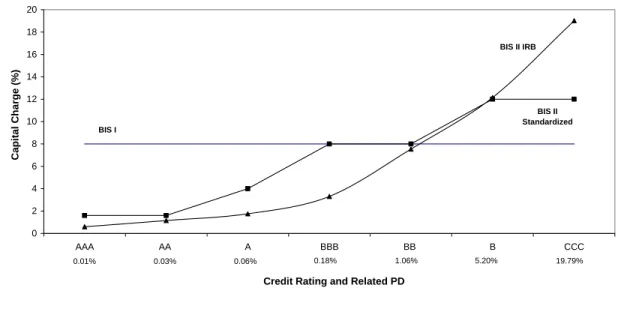
Figure 5 below shows how sensitive (especially compared to Basel I) the resulting IRB capital charge is to a corporate borrower’s credit rating/PD. As can be deduced, loans to highly rated corporates are expected to benefit from Basel II (in terms of incurring a lower capital charge), while low rated loans will be significantly penalized.
Figure 5: Comparison of Capital Requirements under Different Basel Approaches34
33
This effectively corresponds to a one in 1,000 chance that the bank’s credit losses over the next year will exceed the regulatory minimum capital.
34
Uses IRB formula for corporate exposures and assumes an LGD of 45%, an EAD of 100% and effective maturity of 2.5 years. The calibrations of credit ratings to PDs are taken from published default rates for unsecured senior debt by Standard and Poors.
0 2 4 6 8 10 12 14 16 18 20 AAA AA A BBB BB B CCC
Credit Rating and Related PD
Capi tal C ha rge (%) BIS II IRB BIS II Standardized BIS I 0.01% 0.03% 0.06% 0.18% 1.06% 5.20% 19.79%
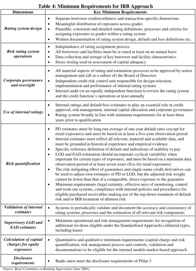
Most asset classes can be treated under one of two approaches: Foundation or Advanced IRB (see Table 3 below). Under the former, banks generally provide their own PD estimates and rely on supervisory estimates for other risk components35. Under the latter, banks provide their own estimates for most/all (depending on the asset class) risk components, subject to meeting minimum standards. However, the same risk-weight functions by asset class must be used for both approaches to derive capital requirements. Once a bank adopts an IRB Approach for part of its holdings, it is expected to extend it across the entire banking group via a phased rollout. The bank’s implementation plan must specify the extent and timing of the roll-out, and must be agreed with the supervisors. Some exposures in non-significant business units and asset classes (or sub-classes in the case of retail) that are deemed immaterial may be exempt from the requirements subject to supervisory approval; these will follow the Standardized Approach for determining capital requirements. Once the bank has adopted an IRB Approach, it is expected to continue to use it – a voluntary return to another approach is permitted only in extraordinary circumstances and must be approved by the supervisor. To be eligible for the IRB Approach, banks must demonstrate to their supervisors that they meet certain minimum requirements at the outset and on an on-going basis. These requirements apply (with some exceptions) across all asset classes and IRB approaches, and are summarized in Table 4 below. However, during the three- year transition period following implementation of the framework, a few specific requirements36 can be relaxed subject to supervisory discretion.
35
For example, under the IRB Foundation Approach, senior and subordinate claims on corporates, sovereigns and banks are assigned an LGD of 45% and 75% respectively, while the effective maturity for corporate exposures is 2.5 years. The comprehensive formula for credit risk mitigation also applies. 36
For example, the minimum five year period to collect data for PD estimation for corporate, sovereign and bank exposures, as well as the minimum three year period to demonstrate the use of a rating system that is broadly in line with minimum requirements for corporate, bank, sovereign and retail exposures.
Table 3: Classification and Treatment of Exposures under the IRB Approach
Asset Classes
Asset Sub-Classes /
Categories IRB Approach Formula for Risk-Weighted Assets
Standard corporate Foundation or Advanced Corporate formula
SMEs Foundation or Advanced Corporate formula with firm-size adjustment
Eligible purchased
receivables Foundation or Advanced
Corporate formula with different (top-down) procedure for deriving PD and LGD; firm-size adjustment might also
apply; additional adjustment in formula to account for dilution risk
Corporate
Specialized Lending (project finance, object
finance, commodities finance, income -producing real estate,
high-volatility commercial real estate)
‘Supervisory slotting criteria’ or Foundation or
Advanced
Separate formula for ‘supervisory slotting criteria’ approach; Corporate formula for Foundation or Advanced
Approach; adjustments to both formulas for high-volatility commercial real estate exposures
Sovereign N/A Foundation or Advanced Same as Corporate formula
Bank N/A Foundation or Advanced Same as Corporate formula Secured by residential
property (e.g. residential mortgages)
No distinction (only one approach)
Separate formula for residential mortgage exposures Qualifying revolving
retail (e.g. credit cards)
No distinction (only one approach)
Separate formula for qualifying revolving retail exposures All other retail
exposures (e.g. consumer loans)
No distinction (only one approach)
Separate formula for other retail exposures
Retail*
Eligible purchased receivables
No distinction (only one approach)
One of the three Retail formulas, depending on composition of receivables; Retail formula with highest capital requirements to be used
for hybrid (mixed) pools; adjustment to selected formula to account for
dilution risk
Equity** N/A Market-based or PD/LGD
Two distinct formulas for market-based approach (simple risk weight or
internal models method); separate formula for PD/LGD approach
Source: Basel Committee on Banking Supervision (June 2004).
* Applies to each identified pool of exposures ( as opposed to individual exposures).
Table 4: Minimum Requirements for IRB Approach
Dimensions Key Minimum Requirements
Rating system design
• Separate borrower creditworthiness and transaction-specific dimensions
• Meaningful distribution of exposures across grades
• Plausible, consistent and detailed rating definitions, processes and criteria for assigning exposures to grades within a rating system
• Written documentation of rating system design, default and loss definitions etc.
Risk rating system operations
• Independence of rating assignment process
• All borrowers and facilities must be re-rated at least on an annual basis
• Data collection and storage of key borrower and facility characteristics
• Stress testing used in assessment of capital adequacy
Corporate governance and oversight
• All material aspects of rating and estimation processes to be approved by senior management and (all or a subset of) the Board of Directors
• Independent credit risk control unit responsible for design/selection, implementation and performance of internal rating systems
• Internal audit (or an equally independent function) to review the rating system and the credit function’s operations at least annually
Use of internal ratings
• Internal ratings and default/loss estimates to play an essential role in credit approval, risk management, internal capital allocation and corporate governance
• Rating system broadly in line with minimum requirements for at least three years prior to qualification
Risk quantification
• PD estimates must be long-run average of one-year default rates (except for retail exposures) and must be based on at least a five-year observation period
• Internal estimates must reflect all relevant, material and available data, and must be grounded in historical experience and empirical evidence
• Specific reference definition of default and indications of inability to pay
• LGD and EAD estimation should incorporate cyclical variability when important for certain types of exposures, and must be based on a minimum data observation period of at least seven years (five for retail exposures)
• The risk-mitigating effect of guarantees and single -name credit derivatives can be used to adjust own estimates of PD or LGD, but the adjusted risk weight cannot be lower than that of a comparable, direct exposure to the guarantor
• Minimum requirements (legal certainty, effective ness o f monitoring, control and work-out systems, compliance with internal policies and procedures) for eligible purchased receivables making use of the top-down treatment of default risk and/or IRB treatment of dilution risk
Validation of internal estimates
• Systems to periodically validate and document the accuracy and consistency of rating systems, processes and the estimation of all relevant risk components
Supervisory LGD and EAD estimates
• Minimum operational and risk management requirements for recognition of additional (to those eligible under the Standardized Approach) collateral types, including leases
Calculation of capital charges for equity
exposures
• Quantitative and qualitative minimum requirements (capital charge and risk quantification, risk management process and controls, validation and documentation) to be eligible for the internal models market-based approach
Disclosure
requirements • Banks must meet the disclosure requirements of Pillar 3
Securitizations
The Basel Committee introduces a separate securitization framework that aims to align regulatory capital treatment to the actual credit risk incurred by such exposures. Banks must apply the framework for determining regulatory capital requirements on exposures that arise from traditional or synthetic securitizations37, or similar structures that contain features common to both. Given the multitude of ways in which securitizations may be structured, their eligibility and related capital treatment must be determined on the basis of economic substance rather than legal form38. An originating bank may exclude (non-retained) securitized exposures from the calculation of risk-weighted assets only if specific operational requirements that ensure true and complete risk transfer are fulfilled. The framework includes a Standardized and an IRB Approach for securitization exposures, depending on the method by which the underlying exposures are treated. The former approach applies ECAI assessments that are generally mapped to risk weights, with specific treatment applied to unrated securitization exposures, credit risk mitigants and early amortization features. The latter approach utilizes three different methods to derive regulatory capital requirements:
• Ratings-Based Approach (RBA) for rated exposures, or where a rating can be inferred (subject to specific operational requirements); the risk weights depend on the external/inferred rating, whether the rating is long- or short-term, the granularity of the underlying pool and the seniority of the position
• Internal Assessment Approach for asset-backed commercial paper-related exposures such as liquidity facilities and credit enhancements; banks can use (subject to specific operational requirements) the ir internal credit assessments of such exposures, which must be mapped to equivalent external credit rating agency ratings in order to determine the appropriate RBA risk weights to use
• Supervisory Formula in all other instances; this is based on five bank-supplied inputs (IRB capital charge had the underlying exposures not been securitized, the tranche’s credit enhancement level and thickness, and the pool’s effective number of exposures and weighted average LGD).
For a bank using the IRB Approach, the maximum capital requirement for its securitization exposures is equal to the IRB capital requirement that would have been assessed against the underlying exposures had they not been securitized.
37 A traditional securitization is a structure where the cash flow from an underlying pool of exposures is used to service at least two different stratified risk positions (“tranches”) reflecting different degrees of credit risk (subordination). Payments to the investor depend upon the performance of the specified underlying exposures (as opposed to being derived from an obligation of the entity originating those exposures) and the type of tranche held. A synthetic securitization shares the same structure as a traditional securitization, but it transfers (in whole or in part) the credit risk of an underlying pool of exposures via the use of credit derivatives or guarantees that serve to hedge the risk of the portfolio.
38
Examples of securitization exposures in this context include direct investments in (or retention of) asset-backed and mortgage-asset-backed securities, as well as the provision of explicit (e.g. credit enhancements) or implicit (e.g. liquidity facilities) support to a securitization transaction.
Pillars 2 and 339
The aims of the supervisory review process of the Basel II framework (Second Pillar) are twofold: to ensure that banks have adequate capital to support all their risks40, and to encourage them to develop and use better risk management techniques. Four key principles of supervisory review are identified by the Basel Committee to complement existing best-practice supervisory guidance such as the Basel Core Principles (BCP). Special emphasis is placed on internal controls and risk management processes as additional (to capital) means of addressing bank risks. Another important aspect of this Pillar is the assessment of compliance with the minimum standards and disclosure requirements of the more advanced methods in Pillar 1, such as the IRB Approach for credit risk.
Three main areas are mentioned as being particularly suited to treatment under Pillar 2:
• Risks considered under, but not fully captured by, the Pillar 1 process – for example, credit concentration risk
• Factors not taken into account by Pillar 1 – for example, liquidity risk, interest rate risk in the banking book, business and strategic risks
• Factors external to the bank – for example, business cycle effects.
Although little specific guidance is currently provided for these areas beyond what has already been previously published by the Basel Committee, there is substantial built- in flexibility to incorporate new technical/practical developments going forward.
Pillar 3 develops a set of qualitative and quantitative disclosure requirements to allow market participants to assess, in a consistent and comparable manner, key pieces of information on the institution’s capital adequacy. The aim is to complement the other two Pillars by encouraging market discipline as a ‘counterweight’ to the increased discretion accorded to banks in the estimation of their own capital requirements. Disclosure requirements are either general or specific (i.e. depending on the selected approach), and include information on the scope of application, capital structure and adequacy, and risk exposure and assessment by risk type. Some of those requirements also represent qualifying criteria for the use of particular methodologies or the recognition of particular instruments or transactions in the calculation of regulatory capital.
39
Since the paper focuses primarily on credit risk measurement under Basel II, the discussion of Pillars 2 and 3 issues has been intentionally kept to a minimum; interested readers should refer to the Basel Committee on Banking Supervision (June 2004) for more details.
40
Bank management continues to bear primary responsibility for the capital adequacy assessment process, which is comprised of the following features: board and senior management oversight, sound capital assessment, comprehensive assessment of risks, monitoring and reporting, and internal control review.