Automated Machine Learning
Bayesian Optimization, Meta-Learning & Applicationsa dissertation presented by
Martin Wistuba to
The Department of Computer Science in partial fulfillment of the requirements
for the degree of Doctor of Natural Sciences
in the subject of Computer Science University of Hildesheim Hildesheim, Lower Saxony, Germany
© – Martin Wistuba all rights reserved.
Thesis advisor: Professor Dr. Dr. Lars Schmidt-Thieme Martin Wistuba
Automated Machine Learning
Bayesian Optimization, Meta-Learning & ApplicationsAbstract
Automating machine learning by providing techniques that autonomously find the best algo-rithm, hyperparameter configuration and preprocessing is helpful for both researchers and practi-tioners. Therefore, it is not surprising that automated machine learning has become a very interesting field of research.
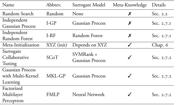
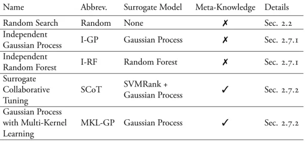
Bayesian optimization has proven to be a very successful tool for automated machine learning. In the first part of the thesis we present different approaches to improve Bayesian optimization by means of transfer learning. We present three different ways of considering meta-knowledge in Bayesian optimization, i.e. search space pruning, initialization and transfer surrogate models. Finally, we present a general framework for Bayesian optimization combined with meta-learning and conduct a comparison among existing work on two different meta-data sets. A conclusion is that in particular the meta-target driven approaches provide better results. Choosing algorithm configurations based on the improvement on the meta-knowledge combined with the expected improvement yields best results.
The second part of this thesis is more application-oriented. Bayesian optimization is applied to large data sets and used as a tool to participate in machine learning challenges. We compare its autonomous performance and its performance in combination with a human expert. At two ECML-PKDD Discovery Challenges, we are able to show that automated machine learning outperforms human machine learning experts.
Finally, we present an approach that automates the process of creating an ensemble of several layers, different algorithms and hyperparameter configurations. These kinds of ensembles are jok-ingly called Frankenstein ensembles and proved their benefit on versatile data sets in many machine learning challenges. We compare our approach Automatic Frankensteining with the current state of the art for automated machine learning on different data sets and can show that it outperforms them on the majority using the same training time. Furthermore, we compare Automatic Franken-steining on a large-scale data set to more than , machine learning expert teams and are able to outperform more than , of them within CPU hours.
Doktorvater: Professor Dr. Dr. Lars Schmidt-Thieme Martin Wistuba
Automated Machine Learning
Bayesian Optimization, Meta-Learning & ApplicationsZusammenfassung
Die Automatisierung des Maschinellen Lernens erlaubt es ohne menschliche Mitwirkung den besten Algorithmus, die dazugehörige beste Konfiguration und die optimale Vorverarbeitung des Datensatzes zu bestimmen und ist daher hilfreich für Anwender mit und ohne fachlichen Hinter-grund. Aus diesem Grund ist es wenig überraschend, dass die Automatisierung des Maschinellen Lernens zu einem populären Forschungsgebiet aufgestiegen ist.
Bayessche Optimierung hat sich als eins der erfolgreicheren Werkzeuge für das automatisierte Maschinelle Lernen hervorgetan. Im ersten Teil dieser Arbeit werden verschiedene Methoden vorge-stellt, die Bayessche Optimierung mittels Lerntransfer auch über Probleme hinweg verbessern kann. Es werden drei Möglichkeiten vorgestellt, um Wissen von zuvor adressierten Problemen auf neue zu Übertragen: Suchraumreduzierung, Initialisierung und transferierende Ersatzmodelle. Schließlich wird ein allgemeines Framework für Bayessche Optimierung beschrieben, welches existierende Meta-lernansätze berücksichtigt und mit schon existierenden Arbeiten auf zwei Meta-Datensätzen ver-glichen. Die beschriebenen Ansätze, die direkt die Meta-Zielfunktion optimieren, liefern tendenziell bessere Ergebnisse. Die Wahl der Algorithmuskonfiguration basierend auf Meta-Wissen kombiniert mit der zu erwartenen Verbesserung erweist sich als beste Methode.
Der zweite Teil der Arbeit ist anwendungsorientierter. Bayessche Optimierung wird im Rahmen von Wettbewerben auf großen Datensätzen angewandt, um Algorithmen des Maschinellen Lernens zu optimieren. Es wird sowohl die eigenständige Leistung der automatisierten Methode als auch die Leistung in Kombination mit einem menschlichen Experten bewertet. Durch die Teilnahme an zwei ECML-PKDD Wettbewerben wird gezeigt, dass das automatisierte Verfahren menschliche Konkurrenten übertreffen kann.
Abschließend wird eine Methode vorgestellt, die automatisch ein mehrschichtiges Ensemble er-stellt, welches aus verschiedenen Algorithmen und entsprechenden Konfigurationen besteht . In der Vergangenheit hat sich gezeigt, dass diese Art von Ensemble die besten Vorhersagen liefern kann. Die beschriebende Methode zur automatisierten Erstellung dieser Ensemble wird mit Hilfe von Datensätzen mit existierenden Konkurrenzansätzen verglichen und erreicht innerhalb derselben Zeit auf der Mehrzahl der Datensätze bessere Ergebnisse. Diese Methode wird zusätzlich mit . Teams von Experten des Maschinellen Lernens auf einem größeren Datensatz verglichen. Es zeigt sich, dass die automatisierte Methodik schon innerhalb von CPU Stunden bessere Ergebnisse liefert als . der menschlichen Teilnehmer des Wettbewerbs.
Contents
I
Introduction and Basics
Introduction
. Overview . . . . Main Contributions . . . . Published Works . . .
Problem Definition & Related Work
. Problem Definition . . . . Standard Techniques for Configuration Optimization . . . . Bayesian Optimization . . . . Meta-Learning . . . . Acquisition Functions . . . . Gaussian Processes . . . . Surrogate Models . . . . Further Related Work . . .
Meta-Data Sets & Experimental Setup
. Meta-Data Sets . . . . Experimental Details . . .
II
Meta-Learning for Bayesian Optimization
Surrogate Model-Free Hyperparameter Optimization
. Contributions . . . . A New Evaluation Metric . . . . Surrogate Model-free Optimization . . . . On a Distance Measure Between Data Sets . . . . Experimental Evaluation . . . . Conclusion . . .
Hyperparameter Search Space Pruning
. Introduction . . . . Pruning the Search Space . . . . Experimental Evaluation . . .
. Conclusion . . .
Hyperparameter Optimization Initialization
. Introduction . . . . Learning Initializations . . . . Experimental Evaluation . . . . Conclusion . . .
Two-Stage Transfer Surrogate Model
. Scalable Two-Stage Transfer Surrogate Framework . . . . Experimental Evaluation . . . . Conclusion . . .
Hyperparameter Optimization Machines
. Hyperparameter Optimization Machines . . . . Adaptive Hyperparameter Transfer Learning with Plain Surrogates . . . . Experimental Evaluation . . . . Conclusion . . .
Conclusion
III
Applied Bayesian Optimization
Distributed Hyperparameter Optimization & Applications
. easyOpt . . . . Experimental Evaluation . . . Automatic Frankensteining . Introduction . . . . Related Work . . . . Background . . . . Automatic Frankensteining . . . . Experimental Section . . . . Conclusions . . . Conclusion
Appendix A Look-Up Tables for SMFO
References
Index
Listing of figures
. Random search works better than grid search for problems with low effective con-figuration dimensionality. . . . In this example, we demonstrate Bayesian optimization by minimizing the
func-tionf(x)=sin(x)+sin(x). At the bottom the acquisition function is plotted and the
cross (×) indicates its global maximum. The predictive posterior distribution is visualized by plotting the mean and standard deviation. Starting with three obser-vations (◦), the response function is approximated. The value with highest expected utility (in this case expected improvement) is selected for the next evaluation. This process is continued and as we see, we find values close to the optimum quickly. . Different acquisition functions with different settings are compared on our
previ-ous example. All acquisition functions have maximums in the same areas but the global maximum might be different. . . . Left: The number of times each hyperparameter configuration has been the best
configuration on the data sets. There is no configuration that has not been best on any data set at least once. Right: The average rank by configuration over all data sets. Unsurprisingly, the higher the number of iterations, the better the configuration on average. . . . The classification error of the AdaBoost classifier on multiple data sets. On many
data sets we can observe that the performance increases with a growing number of iterations. The visualization of all data sets is available athttp://www.hylap.
org/meta_data/adaboost/. . .
. In this plot we visualize which specific configuration has been best on how many of the data sets. There are clear regions of good algorithm configurations. . . . . In this plot we plot the average rank each configuration has achieved over all
data sets. The smaller the better. Unsurprisingly, we see parallels to Figure .. . . . The classification error of the SVM classifier on multiple data sets. The
visualiza-tion of all data sets is available athttp://www.hylap.org/meta_data/svm/. . . . . The classification error of the SVM classifier on multiple data sets. The
visualiza-tion of all data sets is available athttp://www.hylap.org/meta_data/svm/. . . . . The classification error of the SVM classifier on multiple data sets. The
visualiza-tion of all data sets is available athttp://www.hylap.org/meta_data/svm/. . . .
. The classification error of the SVM classifier on multiple data sets. The visualiza-tion of all data sets is available athttp://www.hylap.org/meta_data/svm/.
. . . . This plot presents the number of times each algorithm had a hyperparameter
con-figuration that yield the best classification performance. Support Vector Machines and Random Forests are among the best classifiers. . . . Average difference between the best and worst hyperparameter configuration per
algorithm. Obviously, optimizing the hyperparameters make a huge difference. In many cases a well-tuned algorithm can outperform any other algorithm with random configurations. . . . AUC-ADTM is the area under the loss curves. Since Method is converging
slower than Method , its AUC-ADTM is larger. . . . Metric multidimensional scaling of a distance metric using Euclidean distance on
the meta-features (left) and Equation (.) using only the first four hyperparame-ter configurations recommended by Average SMFO (right). The shown response functions are that from an AdaBoost classifier. The meta-features used are de-scribed in Section .. . . . Development of the average rank among different hyperparameter tuning
strate-gies with increasing number of trials. NN-SMFO shows strong performance es-pecially on the SVM meta-data set. . . . Development of the average distance to the global minimum with increasing
num-ber of trials. RC-GP quickly finds the best configuration on the AdaBoost meta-data set. NN-SMFO provides good results on the AdaBoost meta-meta-data set and the best results on the SVM meta-data set. . . . Running time of the various optimization strategies for the AdaBoost meta-data
set in milliseconds on a logarithmic scale. . . . Pruning is an orthogonal contribution to Bayesian optimization. Nevertheless, we
compare a pruned independent Gaussian process to many current state of the art optimization strategies without pruning. . . . Average rank and average distance to the minimum for I-GP on the SVM
meta-data set. . . . Average rank and average distance to the minimum for I-RF on the SVM
meta-data set. . . . Average rank and average distance to the minimum for SCoT on the SVM
meta-data set. . . . Average rank and average distance to the minimum for MKL-GP on the SVM
meta-data set. . . . Average rank and average distance to the minimum for I-RF and I-GP on the Weka
meta-data set. . .
. Development of the ADTM for increasing number of initial hyperparameter con-figurations on both meta-data sets. Our proposed strategies LI and aLI are outper-forming the state of the art initialization strategies (RBI/NBI) and state of the art surrogate models that transfer knowledge from previous experiments (SCoT and MKL-GP). . . . Impact of an initialization with five hyperparameter configurations on the long
term optimization for I-GP (a surrogate model that does not use information from previous experiments on other data sets). Our proposed strategies LI and aLI are outperforming alternative initialization strategies on both meta-data sets. . . . Impact of an initialization with five hyperparameter configurations on the long
term optimization for I-RF (a surrogate model that does not use information from previous experiments on other data sets). Our proposed initialization strategy LI is outperforming the state of the art on both meta-data sets. . . . Impact of an initialization with five hyperparameter configurations on the long
term optimization for SCoT (a surrogate model that transfers knowledge from previous experiments to the new data set). Our proposed initialization strategy LI is outperforming the state of the art on both meta-data sets. . . . Impact of an initialization with five hyperparameter configurations on the long
term optimization for MKL-GP (a surrogate model that transfers knowledge from previous experiments to the new data set). Our proposed initialization strategy LI is outperforming the state of the art on AdaBoost meta-data sets. We acknowledge that NBI provides better results for the SVM meta-data set. . . . Comparison of the performance development of four different surrogate models
that are all initialized with five LI hyperparameter configurations. RF is a surrogate model that does not transfer knowledge between data sets but yet performs best only due to the LI initialization strategy. Hence, current state of the art surrogate models that transfer knowledge between data sets do not seem to achieve better results if one uses a initialization strategy instead. . . . The proposed framework for our scalable transfer surrogate based on Gaussian
processes. A Gaussian process is learned per data set and they are finally combined in a weighted sum. . . . Our proposed transfer surrogate model TST-R provides the best performance with
respect to both evaluation measures for the task of hyperparameter optimization. For both metrics, the smaller the better. . . . Our approach TST-R also outperforms the competitor methods for the task of
combined algorithm selection and hyperparameter optimization. Surrogate mod-els that use Gaussian processes that train over the whole meta-data are not feasible for this data set. Therefore, we consider I-GP and I-RF with meta-learning ini-tialization. . .
. TST is clearly outperforming the state of the art that is training a single Gaussian process on the full meta-data with respect to scalability. FMLP, which is based on a neural network, has a training time that is linear in the number of data sets, similar to TST. . . . First row: Hyperparameter response functions of the current data set where we
want to find the best hyperparameter configurations and of three data sets which have been investigated before (meta-knowledge). Second row: Sequential process of AHT. One can clearly see the positive impact of the transfer function on the hyperparameter configuration selection in unexplored areas. In all plots: the lower the better. . . . Our proposed method AHT outperforms seven competitor methods with respect
to all three evaluation metrics. . . . AHT with two different surrogate models achieves the best ADTM on the Weka
meta-data set but the combination with a Gaussian process leads to finding optimal hyperparameter configurations in more cases. . . . Strategies based on transfer surrogates are the slowest among all investigated
meth-ods. AHT provides the best performance for a reasonable time overhead. . . . Distribution over all hyperparameter configurations for different algorithms of the
data setbanana. . . . Selection frequency of evaluating the performance of a hyperparameter
configu-ration for a specific hyperparameter configuconfigu-ration. If the value is higher than the uniform distribution, this algorithm was preferred by the optimization strategy. . . The server first registers at the RMI registry. Clients are then able to access
refer-ences to the remote objects. This allows to finally invoke the remote methods. . . . The library contains two main classes. The abstract class EasyOpt manages the
communication with the RMI registry, the class implementing Hyperparame-terOptimization manages the communication between server and client. . . . The server first binds the remote object’s stub to the RMI registry. Now, clients can
lookup the stub and join the optimization. Each client is now sequentially asking for a configuration, evaluates it and reports the result. As soon as the optimization is finished, the server waits until all results are gathered. Then it unbinds the stub from the RMI registry and finishes the process. . . . Intermediate feature backward selection results. Location-aware features provide
huge improvements. . . . This plot visualizes the relative relevance of all features used. The higher the score,
the more often the feature was used for building a tree. Location-aware features prove to be highly predictive. . . . Searching for a good hyperparameter configuration with cores in parallel. The
public leaderboard score is shown for some of the best hyperparameter configura-tions on our validation set. . . . Searching for a good hyperparameter configuration with cores in parallel for
the Network Traffic Classification Challenge. . .
. The final framework consists of two main layers. The first layer learns models on the original data. The estimated models are then ensembled by algorithm family. The resulting predictions lead to our meta-features that are used in the second main layer. Again, models are trained, this time on the meta-features. Finally, all models are ensembled to a single prediction vector. . . . Our approach Automatic Frankensteining is only beaten on data sets by
Auto-WEKA and only by auto-sklearn and hence provides the better solution for the majority of data sets. . . . Automatic Frankensteining (bottom) achieves within hours already a very small
loss on the private leaderboard, outperforming the automated machine learning baselines WEKA (top) and auto-sklearn (middle) as well as the majority of hu-man participants. The dotted lines indicate the perforhu-mane of the Random Forest Benchmark, the top and top of the participants. . .
List of Algorithms
Bayesian Optimization . . . AUC-ADTM Optimizing Sequence . . . Average SMFO . . . Nearest Neighbor AUC-ADTM Optimal Sequence . . . Prune . . . Bayesian Optimization with Pruning . . . Learning Hyperparameter Optimization Initialization . . . Scalable Gaussian Process Transfer Surrogate Framework . . . Hyperparameter Optimization Machines . . . Training the Model Selection Component . . . Bagged Ensemble . . .
To the people who have made me who I am today.
Acknowledgments
Foremost, I want to thank Lars for supervising me over all these years. The fruitful environment he provided for me allowed me to follow my studies but also gave me the freedom to look beyond my own field of research.
I also want to thank Prof. Dr. Pavel Brazdil. Meeting him in person at the ECML-PKDD and and his acknowledgments of our work has been a big motivation. In particular his contribu-tions and feedback to our journal paper and this thesis was very helpful and is very much appreciated. I am grateful to Josif who guided me when I was lost and lacking a research topic. He introduced me to time-series classification, taught me the basics of successful academic writing and is a good friend apart from work and research. Furthermore, he supported me during the project together with Panasonic which I really appreciate.
A special gratitude goes to Nico. Besides the research topic, we have many things in common and it is fun talking with him about research, the lab’s daily life and other topics.
I am grateful to my siblings Stefanie and Oliver and my parents who supported me during my entire life and have been a reliable constant.
I am also very grateful to Kathrin. She was always able to contribute to hard mathematical questions that arose over the past years.
With a special mention to Rasoul, a really nice person who introduced me to active learning and his interesting culture. To Carlotta, my office mate throughout my studies who provided me a silent and calm environment.
And finally, last but by no means least, also to everyone else at ISMLL. It was great sharing lab-oratory with all of you during the last four years.
Thank you all for your encouragement and the great time we had and will have.
Part I
Introduction and Basics
1
Introduction
Algorithm selection and hyperparameter optimization are omnipresent problems for researchers and practitioners. The selection of an algorithm for a specific problem and furthermore the respective hyperparameter configuration has a crucial impact on the quality of the final predictions. Algorithm selection is a well-studied problem that is not limited to machine learning but also finds application in artificial intelligence and operations research. The most conventional method for selecting the algorithm is usually based on the practitioner’s past experience. The hyperparameters are then usually tuned using a combination of manual search and grid or random search. This has two drawbacks. First, inexperienced researchers will have difficulties in choosing the right combination of algorithm and hyperparameter configuration. Second, finding the best hyperparameter configuration by using a grid search will be a time-consuming task. For larger data sets and more advanced algorithms, only few hyperparameter evaluations are feasible with respect to the whole search space.
Recent research proposes automatic algorithm selection and hyperparameter optimization as a solution for these problems. There are methods that need less computational time than manual or grid search and additionally find better hyperparameter configurations than human domain ex-perts,. Recently, a program for combined algorithm selection and hyperparameter optimization was published for the well-known data mining tool Weka. The current direction of research tries to mimic the optimization behavior of human experts. The information of past optimization processes is transferred to current optimization processes. This is done either by initializing the opti-mization process with configurations that performed well on previous experiments,or by using specific machine learning models that predict the performance of an algorithm and hyperparameter
configuration on the current problem based on previous results,,,.
. Overview
This thesis focuses on improving the current state of the art in algorithm selection and hyperparam-eter optimization. The problem is formally defined in Chapter and the current state of the art is discussed. Chapter is used to explain how we created the meta-data sets and the experimental setup. In the chapters to we present different approaches that accelerate the search by means of meta-knowledge. In the final chapters and we compare the state of the art against human machine learning experts. We discuss our results in the ECML-PKDD challenges and how to create complex ensemble methods autonomously.
. Main Contributions
In this thesis we present different techniques that simulate the human behavior of hyperparameter optimization. In the following, we give an overview of these techniques.
.. Hyperparameter Search Space Pruning
Pruning techniques are a typical way of accelerating searches in general. However, pruning has not been applied to hyperparameter optimization yet. In Chapter we propose to discard regions of the search space that are unlikely to contain better hyperparameter configurations. We do so by transferring knowledge from past experiments on other data sets as well as taking into account the evaluations already done on the current data set.
.. Two-Stage Transfer Surrogate Model
Bayesian optimization is a global optimization method that has been proposed for automated ma-chine learning. One of the typical ideas of using knowledge about various problems in Bayesian optimization is the use of transfer surrogate models. Surrogate models are able to predict the loss for each configuration and are employed to select interesting configurations for evaluation. We propose a specific transfer surrogate model in Chapter . This surrogate consists of two stages. On the first stage, several Gaussian processes are created that reconstruct the response function for each data set. On the second stage, this meta-knowledge is combined based on the similarity between each data set to the new data set. We compare it to the state of the art and show that it provides very competitive results and easily scales to large meta-data sets.
.. Meta-Target Driven Optimization
Traditional machine learning methods such as regression or classification have natural evaluation measures such as the squared error or the classification error. A machine learning model is typically trained by minimizing a loss function which is directly derived from the given evaluation measure. The Bayesian optimization methods for hyperparameter optimization as proposed so far do not follow this principled way of minimizing the loss of interest. During my studies I developed different ways of finding this principled way.
In Chapter we present the very first idea of optimizing directly for the evaluation measure. We propose to choose hyperparameter configurations based on a cost function that depends on the performance of the respective configuration on other problems. The evaluations on the new data set are only taken into account to predict the similarity between the current and former problems. This simple idea is the first step into the right direction but provides some disadvantages. Its biggest disadvantage is that the configuration candidates are limited to those used in the meta-data.
We get rid of this restriction in Chapter . We formalize a meta-loss for hyperparameter optimiza-tion. This loss is used to compute a meta-initialization for hyperparameter optimization methods which determines which configurations are tried first.
Our final contribution in this direction is presented in Chapter . The meta-loss defined in Chapter is used directly within the hyperparameter configuration acquisition procedure. Thus, we achieve an effect that can be considered as a soft meta-initialization. But in comparison to a meta-initialization, the meta-knowledge about previous data sets and the new data set is considered for each hyperparameter configuration choice. The impact of the meta-knowledge about previous data sets vanishes over time since this knowledge has been exploited and only the knowledge from the new data set is used. This is an intended result that all transfer surrogates fail to achieve because they consider meta-knowledge equally, independent on the progress of the optimization process.
.. Applications
In most of our results we restrict ourselves to lab experiments. However, in Chapter and we conduct experiments on large data sets and compare to human expert performance.
We first explain a very elegant way of using Bayesian optimization in distributed systems with remote method invocation (RMI) in Chapter . Our implemented system is finally evaluated in the participation in two ECML-PKDD Discovery Challenges (European Conference on Machine Learning and Principles and Practice of Knowledge Discovery). In the Bank Card Usage Prediction Challenge, we combined Bayesian optimization with human interaction and achieved the first place. In the Network Traffic Classification Challenge, we participated without human interaction, letting
Bayesian optimization do the job for us and placed third, outperforming many human competitors. In Chapter we describe a way of creating complex ensembles autonomously by using Bayesian optimization as the core optimization method. We compare our performance to the state of the art in automated machine learning on UCI data sets and compare to more than , human machine learning experts by participating in one Kaggle challenge. In an extensive evaluation we can show that we outperform the state of the art in automated machine learning and most human machine learning experts.
. Published Works
The different chapters are mostly based on published peer-reviewed work,,,,,,.
Chapter Wistuba, M., Schilling, N., & Schmidt-Thieme, L. (). Sequential model-free hy-perparameter tuning. In IEEE International Conference on Data Mining, ICDM , Atlantic City, NJ, USA, November -, (pp. -).
Chapter Wistuba, M., Schilling, N., & Schmidt-Thieme, L. (). Hyperparameter search space pruning - A new component for sequential model-based hyperparameter optimization. In Machine Learning and Knowledge Discovery in Databases - European Conference, ECML-PKDD , Porto, Portugal, September -, , Proceedings, Part II (pp. -).
Chapter Wistuba, M., Schilling, N., & Schmidt-Thieme, L. (). Learning hyperparameter optimization initializations. In IEEE International Conference on Data Science and Advanced Analytics, DSAA , Campus des Cordeliers, Paris, France, October -, (pp. -). Chapter Wistuba, M., Schilling, N., & Schmidt-Thieme, L. (). Two-stage transfer surro-gate model for automatic hyperparameter optimization. InMachine Learning and Knowledge Discov-ery in Databases - European Conference, ECML-PKDD , Riva del Garda, Italy, September -, , Proceedings, Part I (pp. -).
Chapter Wistuba, M., Schilling, N., & Schmidt-Thieme, L. (). Hyperparameter opti-mization machines. In IEEE International Conference on Data Science and Advanced Analytics, DSAA , Montreal, QC, Canada, October -, (pp. -).
Chapter Wistuba, M., Duong-Trung N., Schilling, N., & Schmidt-Thieme, L. (). Bank card usage prediction exploiting geolocation information. CoRR, abs/..
Chapter Wistuba, M., Schilling, N., & Schmidt-Thieme, L. (). Automatic Franken-steining: Creating complex ensembles autonomously. Accepted at the SIAM International Conference on Data Mining, SDM , Houston, Texas, USA, April -, .
2
Problem Definition & Related Work
In this chapter, we formally define the problem addressed in this thesis and the notation used. We review how configurations of algorithms are typically optimized in machine learning and recent progresses achieved with Bayesian optimization.
. Problem Definition
When tackling a machine learning problem, let us say classification, a machine learning expert has to make many decisions. One aspect of her decision process is the selection of the algorithm and its parameters. Unfortunately, most algorithms have many parameters that need to be defined by the machine learning expert before training the classifier. To distinguish them from model parameters, which are estimated during the learning procedure, we call themhyperparameters. Most hyperpa-rameters define the model complexity (e.g. number of nodes in a neural network, depth of a tree, regularization parameters) or have influence on the learning procedure (e.g. learning rate, momen-tum, number of iterations). These specific parameters have high impact on how good an algorithm performs. Hence, the algorithm and its hyperparameter need to be chosen in combination. This thesis will present methods that can autonomously find the right combination of algorithm and its configuration.
In the following, we formally define the problem ofconfiguration optimizationand the notation used throughout the thesis. For notational convenience we assume that there is only one possible learning task applicable for a data set. We denote the space of all data sets asDand the space of all
models asM.X is the space of all configurations. Then, we define a general learning algorithmA as a mapping
A:D × X → M . (.)
The configurationx ∈ X encodes the configuration, i.e. it defines which machine learning algo-rithm and the hyperparameter configuration is selected. Further properties that might be included inX are preprocessing, feature selection or feature engineering.
Given a data setD ∈ D, which is partitioned into Dtrain andDvalid, and a configuration x ∈
X, the general learning algorithm A estimates a prediction modelM ∈ M(x). This model is estimated by minimizing a loss functionL(e.g. residual sum of squares) which is penalized with a regularization termR(e.g. Tikhonov regularization) with respect to the training dataDtrain. That is,
A(D,x) =arg min
M∈M(x)
L(M,Dtrain) +R(M) . (.)
The task in this thesis is to find the configurationx∗that leads to a prediction model which minimizes the loss on the validation partitionDvalid. Formally,
x∗=arg min
x∈X
L(A(Dtrain,x),Dvalid) =arg min
x∈X
fD(x) . (.)
The functionfD : X →Rwith
fD(x) =L(A(Dtrain,x),Dvalid) (.)
is theresponse functionof data setD. In many applications, the configuration spaceX equals the hy-perparameter space of a single algorithm and hence, we call this task alsohyperparameter optimization and the configurations hyperparameter configurations.
For the sake of demonstration, we consider the problem of optimizing the hyperparameters of classifiers in this thesis. Thus, the response function fD maps a configuration to the classification
error. This is no limitation, but shall help the reader to understand the concepts.
. Standard Techniques for Configuration Optimization
Evaluating the response functionfDat a single point involves training a machine learning model
which is a time-consuming task. Hence, the minimization offDcannot be achieved with standard
optimization techniques. A very common technique is grid search. Given the configuration space,
X =X×. . .× XP , (.)
Response Function Sensitiv e Parameter Insensitiv e Par ameter Grid Search Sensitive Parameter Insensitiv e P ar ameter Random Search Sensitive Parameter Insensitiv e P ar ameter
Figure 2.1:Random search works better than grid search for problems with low effective configuration dimensionality.
a set ofki values is chosen for each dimension.
Gi ={x, . . . ,xki}, x, . . . ,xki ∈ Xi (.) Then, all configurations in
G=G×. . .×GP (.)
are evaluated and the best performing is selected.
An alternative to grid search is random search. Similarly to grid search, the upper and lower bounds per dimension need to be defined. Then, configurationsxare sampled uniformly at random according to
xi ∼ U
(
bmini ,bmaxi ) , (.)
wherebmin
i andbmaxi are the lower and upper bound in the i-th dimension, respectively. This method
works well, in particular if the algorithm has a low effective configuration dimensionality. The reason for this is that in many problems some dimensions are insensitive to changes.
It try to explain this at the example given in Figure .. It shows a two-dimensional response function where only one dimension is sensitive to changes. Thus, the effective dimensionality is just one. Applying a grid search will lead to many redundant function evaluations. In fact, only four different values of the sensitive parameter are tested. Otherwise, random search efficiently uses every evaluation and tests sixteen different values of the sensitive parameter.
. Bayesian Optimization
Both, grid and random search, are stateless optimization techniques which do not take previous evaluations offinto account. Bayesian optimizationcan be used to overcome this disadvantage. Considering the choice of algorithm configurations as a black-box global optimization problem as defined in Equation ., Bayesian optimization can be used for finding optimal configurations automatically.
Bayesian optimization consists of two components, a surrogate model and an acquisition func-tion. We collect all evaluations off in theobservation history
H={(x,f(x)),(x,f(x)), . . .} . (.) A surrogate model provides a distributionp(f∗|x∗,H)over response function valuesf∗ ∈Rgiven a configuration x∗ ∈ X and for a given observation history H ∈ X ×R. We assume that the predictive posterior distribution of a surrogate model is Gaussian distributed with meanmf|Hand
covarianceΣf|H.
p(f∗|x∗,H) =N(f∗|mf|H(x∗),Σf|H(x∗,x∗)) (.) The acquisition functionaevaluates configurations based on their expected utility. Given a utility functionuf, the acquisition is determined by
a(x∗,p(f∗|x∗,H)) = E[uf(x∗)|x∗,H ] (.) = ∫ uf(x∗)p(f∗|x∗,H)df∗ . (.)
The configuration with highest expected utility
x=arg max
x∗∈X
a(x∗,p(f∗|x∗,H)) (.)
is evaluated next. While the acquisition function introduces a further optimization problem, the evaluation ofais much faster than the evaluation off.
Algorithm outlines Bayesian optimization for minimizing the functionfand Figure . visu-alizes the optimization process. In each iteration,fis approximated by the surrogate model using the observation historyH. The acquisition functionafinds a trade-off between exploitation and exploration and determines the next configurationx∗. This configurationx∗ is evaluated and the new observation is added to the observation history H. After a convergence criterion is met, the best performing configuration is returned. Possible convergence criteria are a time budget or that
● ● ● ● ● ● ● ● ● ● ● ● ● ● ● ● ● ● ● response function observations posterior mean posterior mean +/− stdev
acquisition function next point
Figure 2.2:In this example, we demonstrate Bayesian optimization by minimizing the functionf(x)=sin(x)+sin(x). At the bottom the acquisition function is plotted and the cross (×) indicates its global maximum. The predictive posterior distribu-tion is visualized by plotting the mean and standard deviadistribu-tion. Starting with three observadistribu-tions (◦), the response function is approximated. The value with highest expected utility (in this case expected improvement) is selected for the next evalua-tion. This process is continued and as we see, we find values close to the optimum quickly.
the highest score of the acquisition function is below a thresholdε, i.e. max
x∗∈Xa
(x∗,p(f∗|x∗,H))< ε . (.)
Different acquisition functions and surrogate models have been proposed. We will review them in the next sections. We recommend the recent review by Shahriari et al.as an alternative source for information about Bayesian optimization.
. Meta-Learning
A large part of this thesis is focused on accelerating Bayesian optimization by means of meta-learning. Meta-learning dates back to the sand can be considered as an alternative to Bayesian opti-mization because a considerable amount of work on meta-learning focuses on recommending config-urations for algorithms. No consensus on the definition of meta-learning has been reached. Vilalta and Drissidefine meta-learning as follows:
“Meta-learning studies how learning systems can increase in efficiency through expe-rience; the goal is to understand how learning itself can become flexible according to the domain or task under study.”
Algorithm Bayesian Optimization
Input: Configuration spaceX, observation historyH, acquisition functiona. Output: Best configuration found.
: whilenot convergeddo
: Update the surrogate modelp(f∗|x∗,H). : x∗ ←arg maxx∗∈Xa(x∗,p(f∗|x∗,H)) : f∗ ←f(x∗) : H ← H ∪ {(x∗,f∗)} : if f∗ <fminthen : xmin,fmin←x ∗,f∗ : end if : end while : return xmin
A similar definition is given by Brazdil et al.:
“Meta-learning is the study of principled methods that exploit meta-knowledge to obtain efficient models and solutions by adapting machine learning and data mining processes.”
The idea of meta-learning for configuration recommendation is based on a simple assumption. Algorithms show similar performance for the same configuration for similar problems.
In this thesis we will combine the ideas of meta-learning with Bayesian optimization. This accel-erates the search for good configurations. One way of doing this is by using a meta-initialization. For example, consider configurations that have been good on similar problems will be evaluated first. We discuss this idea in Chapter . Another idea is the use of transfer surrogate models. These surrogate models do not only learn from observations of the response function of the current prob-lem but learn across probprob-lems. This idea is explained in detail in Section .. Further ways of using meta-learning are presented in the upcoming chapters.
In this thesis the term meta-knowledge is used frequently. We define it as the common knowl-edge about response functions and data sets. This includes meta-features and response function evaluations for different data sets. Meta-features are data set descriptors. One example is the num-ber of instances in a data set, further examples are given in Section .. Typically, a data scientist has applied the same algorithm for different data sets. Assuming, she gathered observations fromM many data sets, she collected the meta-knowledge
H={(x,fD(x)), . . . ,(x,fD(xN)), . . . ,(x,fDM(x)), . . . ,(x,fDM(xNM))} . (.)
In the following, we use the prefixmetato distinguish between the different levels of machine learning problems. The traditional machine learning problem is to learn some parameters θ on a given data set containing instances with predictors. For the configuration optimization prob-lem, we create meta-data sets consisting of meta-instances with meta-predictors. A meta-data set contains meta-instances(xi,fD(xi)) where fD(xi) is the target and xi are the predictors. These
meta-predictors can be enriched by meta-features.
. Acquisition Functions
As discussed earlier, finding optimal configurations for machine learning algorithms can be consid-ered a global optimization of a functionf where f is an expensive black-box function. Given a set of observationsH, a surrogate model can be computed that provides a distribution overf. The important question is now, how to decide which point of the function to evaluate next. This is done by the acquisition functionathat scores for every point how desirable its evaluation for our mini-mization problem is. Hence, another optimini-mization problem, the maximini-mization ofa, is introduced. Fortunately, the functionais much cheaper to evaluate thanf.
Many different acquisition functions have been proposed to evaluate the expected value offfor a specific argument. Acquisition functions can be categorized into three different classes. Improvement-based policies such as probability of improvementand expected improvementconsider the cur-rently best observation in their decision. Information-based policies aim at reducing the entropy of the posterior distribution around the optimal value
xmin=arg min
x∈X
f(x) . (.)
Examples are Thompson samplingand entropy search,,. The idea of optimistic policies is to minimize the regret during Bayesian optimization. There are various representatives for these poli-cies,,. Furthermore, a combination of different acquisition functions have been proposed. We will review some of the more prominent acquisition functions in the following.
.. Probability of Improvement
Given a functionfto minimize and the observation historyH= (X,f), the best value offobserved so far is
fmin=minf . (.)
The acquisition function called probability of improvement estimates the probability that the value offfor the configurationx∗ is better than currently best valuefmin. Hence, it is based on a
●
●
●
●
response function observations posterior mean posterior mean +/− stdev
PI EI GP−LCB (β=2) GP−LCB (β=0.5)
Figure 2.3:Different acquisition functions with different settings are compared on our previous example. All acquisition functions have maximums in the same areas but the global maximum might be different.
utility function that is if the value offfor the configurationx∗ is better than currently best value fminand otherwise. Formally,
uf(x∗) = f(x∗)<fmin otherwise . (.)
As one can see, the utility function of the probability of improvement does not depend on how much f(x∗)improves overfmin. This leads to a greedy behavior which can be seen in Figure ., where we compare this approach to other acquisition functions. Following the definition in Equation ., probability of improvement can be derived as follows
aPI(x∗,p(f∗|x∗,H)) := E [ uf(x∗)|x∗,H ] (.) = ∫ uf(x∗)p(f∗|x∗,H)df∗ (.) = ∫ fmin −∞ N ( f∗|mf|H(x∗),Σf|H(x∗,x∗))df∗ (.) = Φ(fmin|mf|H(x∗),Σf|H(x∗,x∗)) (.) whereN (·|m, σ)andΦ (·|m, σ)denote the general normal distribution and cumulative distribu-tion funcdistribu-tion with meanmand standard deviationσ, respectively. The predictive posterior
bution of the surrogate modelp(f∗|x∗,H)is defined as
p(f∗|x∗,H) =N(f∗|mf|H(x∗),Σf|H(x∗,x∗)) . (.)
.. Expected Improvement
The expected improvement is the most prominent choice for hyperparameter optimization. Snoek et al. provided experiments that showed that is performing best for our task of configuration optimization. For these two reasons we used this acquisition function in all our experiments.
The difference to the probability of improvement is small but important. Expected improvement considers how much a configuration likely improves over the currently best solution. Formally, the utility for a configurationx∗∈ X is defined as
uf(x∗) =max
{
fmin−f(x∗),} . (.)
Given this utility, the expected improvement for a configurationx∗ is defined as aEI(x∗,p(f∗|x∗,H)) := E [ uf(x∗)|x∗,H ] (.) = ∫ uf(x∗)p(f∗|x∗,H)df∗ (.) = ∫ fmin −∞ ( fmin−f∗)N (f∗|mf|H(x∗),Σf|H(x∗,x∗))df∗ (.) = (fmin−mf|H(x∗))Φ(fmin|mf|H(x∗),Σf|H(x∗,x∗)) + √ Σf|H(x∗,x∗)N(fmin|mf|H(x∗),Σf|H(x∗,x∗)) .(.) Proof. In the following, we will prove the step from Equation (.) to Equation (.). For nota-tional convenience, we will useµ=mf|H(x∗)andσ = Σf|H(x∗,x∗).
∫ fmin −∞ ( fmin−f∗)N(f∗|µ, σ)df∗ (.) = ∫ fmin −∞ f minN(f ∗|µ, σ)df∗− ∫ fmin −∞ f∗N ( f∗|µ, σ)df∗ (.) = fminΦ(fmin|µ, σ)− ∫ fmin −∞ f∗ √ πσexp ( −(f∗−µ) σ ) df∗ . (.)
We can rewrite ∫ fmin −∞ f∗ √ πσexp ( −(f∗−µ) σ ) df∗ (.) = ∫ fmin −∞ (f∗−µ) √ πσexp ( −(f∗−µ) σ ) df∗ + ∫ fmin −∞ µ √ πσexp ( −(f∗−µ) σ ) df∗ (.) = ∫ fmin −∞ (f∗−µ) σ √ πexp ( −(f∗−µ) σ ) df∗+µΦ(fmin|µ, σ) . (.) Then, by substitutingt= f∗σ−µ, we derive
∫ fmin −∞ (f∗−µ) σ √ πexp ( −(f∗−µ) σ ) df∗ (.) = √ π ∫ fmin−µ σ −∞ t·exp ( −t ) dt (.) = ·√π ∫ fmin−µ σ −∞ t·exp ( −t ) dt . (.)
Definingg(t) =e−t/andh(t) =t, we get
√π ∫ fmin−µ σ −∞ ( d dth(t) ) g(h(t))dt . (.)
Integrating by substitution, we obtain √π ∫ ∞ (fmin−µ σ )g(u)du = √π ∫ ∞ (fmin−µ σ )e−u/du (.) = √π [ −e−u/ ]∞ (fmin−µ σ ) (.) = √σ πσexp ( − ( fmin−µ) σ ) (.) = σN(fmin|µ, σ) . (.)
Finally, we can conclude
∫ fmin
−∞ (
fmin−f∗)N(f∗|µ, σ)df∗ (.)
= fminΦ(fmin|µ, σ)−(σN (fmin|µ, σ)+µΦ(fmin|µ, σ)) (.) = (fmin−µ)Φ(fmin|µ, σ)−σN (fmin|µ, σ) . (.)
The utility function in Equation (.) is called improvement and in a similar way applied by other approaches in meta-learning. Leite et al. make use of relative landmarks which estimate the improvement of one configuration over another based on observations on previous problems. We employ this related improvement also in chapters and .
.. Entropy Search
The information-based acquisition functions are inspired by techniques proposed in active learn-ing. The idea is to maximize the information about the location at the current optimal configu-ration
xmin=arg min
x∈X f
(x) . (.)
The utility of a configuration is measured in terms of the change of entropy for the posterior distri-butionp(xmin|H). Thus, the utility function is defined as
uf(x∗) =h
[
xmin|H]−h[xmin|H ∪ {(x∗,f(x∗))}] , (.) whereh[x]is the continuous entropy
h[x] =− ∫
p(x)lnp(x)dx . (.)
The higher the information gain after adding the observation for configurationx∗, the higher the values of the utility function. The acquisition function is then the expected information gain when choosing a configurationx∗: aES(x∗) :=h [ xmin|H]− ∫ h[xmin|H ∪ {(x∗,f∗)}]p(f∗|x∗,H)df∗ . (.) Computing the expected value of the continuous entropy and computing the continuous entropies itself are intractable in practice. Hence, different approximations have been proposed,,.
.. Lower/Upper Confidence Bounds
The GP-UCB acquisition function, is based on the seminal work by Lai and Robbins on the multi-armed bandit problem. The idea is to be very optimistic about the outcome, always ex-pecting the best case scenario. The acquisition function was introduced for function maximization, hence, upper confidence bounds are used
aGP-UCB(x∗,p(f∗|x∗,H)) :=mf|H(x∗) +βt
√
Σf|H(x∗,x∗) , (.)
whereβtis used to balance exploitation and exploration at stept. In case of function minimization, the acquisition function can be redefined by using lower confidence bounds:
aGP-LCB(x∗,p(f∗|x∗,H)) :=−mf|H(x∗) +βt
√
Σf|H(x∗,x∗) . (.)
In contrast to the previous acquisition functions, the GP-UCB/LCB acquisition function requires the optimization of the hyperparameterβt. It has been proven that with high probability GP-UCB
has no regret for specificβt.
. Gaussian Processes
Gaussian processes are the most dominant surrogate model for Bayesian optimization and hence we recapture its definition. For more information, we refer the interested reader to the excellent book by Rasmussen and Williams, entitled Gaussian Processes for Machine Learning.
The regression problem is to model relationships between one dependent variablefiand multiple
independent variablesxi. This relationship is assumed to be described by a latent function
f:X →R . (.)
The functionfis unknown but noisy observations(xi,fi)of this functions are available. The
rela-tionship tofcan be explained by decomposing it into a signal and a noise part
fi =f(xi) +e(xi) , (.)
whereeis the stochastic error. In the context of machine learning, the set of pairs of observations is
also called training data.
X = (x, . . . ,xN) (.)
f = (f, . . . ,fN) (.)
Gaussian process models assume a Gaussian prior onf. Every observationfiis considered to be a
random variable and the joint distribution of allfiis assumed to be multivariate Gaussian distributed:
p(f|X,θ) =N (f|m(X),k(X,X)) . (.) A Gaussian process is completely specified by its mean functionmand its covariance functionkand possibly depends on some parametersθ. In order to predict the labelsf∗for some test instancesx∗, the Gaussian process assumption is thatfandf∗ are jointly Gaussian
p(f,f∗|X,X∗,θ) =N (( f f∗ ) ( m(X) m(X∗) ) , ( Kn K∗ KT ∗ K∗∗ )) , (.) where Kn = K+σnI (.) K∗ = k(X,X∗) (.) K∗∗ = k(X∗,X∗) (.)
for brevity. In this notation,σnis a noise hyperparameter added to the diagonal of the kernel matrix
K=k(X,X). The predictive posterior distribution can be obtained from the joint distribution.
p(f∗|X,f,X∗,θ) =N(f∗|m(X∗) +KT∗K−(f−m(X)),K∗∗−KTK−K∗) (.) From now on we assumem(x) = to simplify the notation.
A typical covariance function used is the squared exponential kernel with automatic relevance determination k(xi,xj ) =exp − dim∑X p= ( xi,p−xj,p ) σ p . (.)
Kernel hyperparametersθ can be estimated and optimized by maximizing the log marginal
hood on the training data which is given by logp(f|X,θ) =− f TK− n f− log|Kn| − N log(π) . (.)
Bayesian optimization requires frequent updates of the Gaussian process. Retraining it completely is computationally expensive and dominated by the inversion of the kernel matrix which is cubic in the number of training instances. Using a little trick, the update can be reduced to squared run time complexity. The kernel matrix is decomposed using the Cholesky decompositionKn =LLT.
Then, the predicted probability distribution for a single instancex∗is
p(f∗|x∗,X,f,θ) =N (f∗|kT∗α,k∗∗−lTl) , (.) with
α = LT\(L\f) (.)
l = L\k∗ , (.)
where\is the operator for solving an equation system. SinceLis a triangular matrix, the equation system can be solved in quadratic time. If now a new instance needs to be added, the triangular matrixLcan be updated by
Lnew= ( L lT l ∗ ) , (.) where l∗ = √ k(x∗,x∗)− ∥l∥+σ y . (.)
Nowαandlcan be recomputed as described in Equation (.) and (.).
. Surrogate Models
In this section, we review the most important surrogate models for Bayesian optimization for con-figuration optimization in machine learning. We distinguish between plain and transfer surrogate models which we define as follows. LetDnew be the data set for which we search for the optimal configurations. Then, a plain surrogate model is one that considers only observations and informa-tion offDnew andDnew. Otherwise, we define transfer surrogate models as those surrogate models
that use information of additional data sets besidesDnew.
.. Plain Surrogate Models Spearmint
Snoek et al. are the first to propose the use of Bayesian optimization for hyperparameter opti-mization in machine learning. They use a Gaussian process as a surrogate model. In their work they investigate different aspects of Bayesian optimization with respect to hyperparameter optimization. They compare different acquisition functions, propose a run-time-aware acquisition function and describe how to run the optimization in parallel.
Sequential Model-based Algorithm Configuration
Hutter et al.propose the use of random forests as a surrogate model. While the original work fo-cuses on the algorithm configuration problem for solvers of hard computational problems (Boolean satisfiability problem (SAT) and mixed integer programming (MIP)), it is currently used in libraries for autonomous machine learning such as auto-sklearnand Auto-WEKA.
.. Transfer Surrogate Models
Transfer surrogate models use meta-knowledge of various data sets. In practice, this usually means nothing else but extending the observation history by adding observations from other data sets. Assuming we have observations fromMmany data sets, we start Bayesian optimization with the non-empty observation history
H={(x,fD(x)), . . . ,(x,fD(xN)),(x, . . . ,fDM(x)), . . . ,(x,fDM(xN))} . (.) Furthermore, various techniques of using meta-features might be considered but often they are simply added to the meta-predictorsx.
Surrogate Collaborative Tuning
Bardenet et al.are the first to propose a transfer surrogate. They show how to learn a single surrogate model over observations from many data sets. Since the same algorithm applied to different data sets leads to loss values that can differ significantly in scale, they recommend tackling this problem using a ranking model instead of a regression model. They finally propose to use SVMRANKwith an RBF kernel to learn a ranking of hyperparameter configurations per data set. The ranker itself does not provide the needed uncertainty estimations. Thus, they finally fit a Gaussian process to the output of the ranker.
Gaussian Process with Multi-Kernel Learning
Yogatama and Mannpropose to train a Gaussian process directly on the meta-data. To overcome the problem of different scales on different data sets, they propose to standardize the loss per data set by removing the mean and scaling to unit variance. Furthermore, they propose a linear combination of a squared exponential kernel with automatic relevance determination (SE-ARD) for points in the same data set and a nearest neighbor kernel for modeling similarities between data sets. They define the kernel as kMKL ( (xi,Dk), ( xj,Dl )) =αI(Dk=Dl)kSE-ARD ( xi,xj ) + (−α)I(Dl∈ N(D))kNN ( xi,xj ) (.) where the SE-ARD kernel is defined as
kSE-ARD ( xi,xj ) =exp − ∑ p ( xi,p−xj,p ) σ p (.)
and the data set similarity kernel as kNN ( xi,xj ) =− Bxi−xj, (.)
whereBmust be chosen such thatkNNis always non-negative andN (D)denotes the set of neigh-bored data sets with respect to a distance function. The distance between two data sets is defined as the Euclidean distance between its meta-features. Meta-features are used only to determine the distance between data sets. They are not used within the kernels. Hence, meta-features are only used to estimate the values ofkNN.
Factorized Multilayer Perceptron
Schilling et al. propose to use a modified multilayer perceptron as a surrogate model. Meta-instances are extended by meta-features and data set indicators. Data set indicators are nothing else butM+ additional binary predictors, one for each data set. The indicator is if the meta-instance belongs to the corresponding data set, otherwise. The modified multilayer perceptron uses a different activation function in the first layer than the standard multilayer perceptron. Instead of using the typical sigmoid activation function, they propose
logistic w+ P ∑ i= wixi+ P ∑ i= P ∑ j=i+ vTi vjxixj (.)