Discrimination in Algorithmic Decision Making: From Principles to Measures and Mechanisms

From Principles to Measures and Mechanisms

A dissertation submitted towards the degree

Doctor of Engineering

of the Faculty of Mathematics and Computer Science of

Saarland University

by

Muhammad Bilal Zafar

Saarbrücken

February, 2019

Chair of the Committee: Prof. Dr. Gerhard Weikum

Reporters

First Reviewer: Prof. Dr. Krishna P. Gummadi

Second Reviewer: Dr. Manuel Gomez Rodriguez

Third Reviewer: Prof. Dr. Sharad Goel, Ph.D.

Fourth Reviewer: Prof. Dr. Paul Resnick, Ph.D.

Academic Assistant: Dr. Rishiraj Saha Roy ii

ALL RIGHTS RESERVED

The rise of algorithmic decision making in a variety of applications has also raised concerns about its potential for discrimination against certain social groups. However, incorporating nondiscrimination goals into the design of algorithmic decision making systems (or, classifiers) has proven to be quite challenging. These challenges arise mainly due to the computational complexities involved in the process, and the inadequacy of existing measures to computationally capture discrimination in various situations. The goal of this thesis is to tackle these problems.

First, with the aim of incorporating existing measures of discrimination (namely, disparate treatment and disparate impact) into the design of well-known classifiers, we introduce a mechanism of decision boundary covariance, that can be included in the formulation of any convex boundary-based classifier in the form of convex constraints. Second, we propose alternative measures of discrimination. Our first proposed measure, disparate mistreatment, is useful in situations when unbiased ground truth training data is available. The other two measures, preferred treatment and preferred impact, are useful in situations when feature and class distributions of different social groups are significantly different, and can additionally help reduce the cost of nondiscrimination (as compared to the existing measures). We also design mechanisms to incorporate these new measures into the design of convex boundary-based classifiers.

Die Vielzahl der Anwendungen, die Algorithmen immer stärker an Entscheidungsprozessen beteiligen, wächst stetig. Dadurch werden Bedenken über die potenzielle Diskrim-inierung bestimmter gesellschaftlicher Gruppen aufgeworfen. Die Aufnahme von Nicht-diskriminierungszielsetzungen bei der Gestaltung algorithmischer Entscheidungs- bzw. Klassifizierungssysteme hat sich jedoch als grosse Herausforderung herausgestellt. Zum einen sind die nötigen Berechnungen komplex und zum anderen sind die existierenden Metriken unzureichend, um Diskriminierung in bestimmten Situationen rechnerisch zu erfassen. Das Ziel dieser Arbeit ist es, diese Problematik anzugehen.

Als erstes stellen wir einen Decision Boundary-basierten Kovarianzmechanismus vor, der genutzt werden kann, um existierende Diskriminierungsmetriken (also Disparate Treatment und Disparate Impact) beim Entwurf von gängigen Klassifizierungsalgo-rithmen einzusetzen. Der Ansatz kann für jeden konvexen Boundary-basierten Klassi-fizierungsalgorithmus in Form konvexer Constraints formuliert werden. Als nächstes definieren wir neue Diskriminierungsmetriken. Unsere erste Metrik namens Disparate Mistreatment kommt in Situationen zum Einsatz, in denen die Referenzdaten nicht zugunsten einer sozialen Gruppe verzerrt sind. Die übrigen beiden Metriken namens Preferred Treatment und Preferred Impact sind für Situationen konzipiert, in denen die Feature- und Klassenverteilungen unterschiedlicher sozialer Gruppen stark voneinander abweichen. Sie können dabei helfen, die Kosten von Nichtdiskriminierung im Vergleich zu bestehenden Metriken zu reduzieren. Wir zeigen ebenfalls, wie diese neuen Metriken in konvexen Boundary-basierten Klassifizierungsalgorithmen genutzt werden können.

Parts of this thesis have appeared in the following publications.

• “From Parity to Preference-based Notions of Fairness in Classification”. M. B. Zafar, I. Valera, M. Gomez-Rodriguez, K. P. Gummadi and A. Weller. InProceedings of the 31st_{Annual Conference on Neural Information Processing Systems (NIPS), Long Beach,}

CA, December 2017.

• “Fairness Beyond Disparate Treatment & Disparate Impact: Learning Classification without Disparate Mistreatment”. M. B. Zafar, I. Valera, M. Gomez-Rodriguez and K. P. Gummadi. InProceedings of the 26th _{International World Wide Web Conference} (WWW), Perth, Australia, April 2017.

• “Fairness Constraints: Mechanisms for Fair Classification”. M. B. Zafar, I. Valera, M. Gomez-Rodriguez and K. P. Gummadi. InProceedings of the 20th _{International} Conference on Artificial Intelligence and Statistics (AISTATS), Fort Lauderdale, FL, April 2017.

Additional publications while at MPI-SWS.

• “A Unified Approach to Quantifying Algorithmic Unfairness: Measuring Indi-vidual and Group Unfairness via Inequality Indices ”. T. Speicher, H. Heidari, N. Grgic-Hlaca, K. P. Gummadi, A. Singla, A. Weller, M. B. Zafar. InProceedings of the 24th_{International Conference on Knowledge Discovery and Data Mining (KDD), London,}

UK, August 2018.

• “Beyond Distributive Fairness in Algorithmic Decision Making: Feature Selection for Procedurally Fair Learning”. N. Grgic-Hlaca, M. B. Zafar, K. P. Gummadi and A. Weller. InProceedings of the 32nd_{AAAI Conference on Artificial Intelligence (AAAI),}

New Orleans, LA, February 2018.

Gummadi and K. Karahalios. InProceedings of the 20th_{ACM Conference on} Computer-Supported Cooperative Work and Social Computing (CSCW), Portland, OR, February 2017.

• “Listening to Whispers of Ripple: Linking Wallets and Deanonymizing Transac-tions in the Ripple Network”. P. Moreno-Sanchez, M. B. Zafar and A. Kate. In

Proceedings on Privacy Enhancing Technologies (PoPETS), 2016.

• “Message Impartiality in Social Media Discussions”. M. B. Zafar, K. P. Gummadi and C. Danescu-Niculescu-Mizil. InProceedings of the 10thInternational AAAI Con-ference on Web and Social Media (ICWSM), Cologne, Germany, May 2016.

• “On the Wisdom of Experts vs. Crowds: Discovering Trustworthy Topical News in Microblogs”. M. B. Zafar, P. Bhattacharya, N. Ganguly, S. Ghosh and K. P. Gummadi. InProceedings of the 19th_{ACM Conference on Computer-Supported Cooperative Work} and Social Computing (CSCW), Portland, OR, February 2016.

• “Strength in Numbers: Robust Tamper Detection in Crowd Computations”. B. Viswanath, M. A. Bashir, M. B. Zafar, S. Bouget, S. Guha, K. P. Gummadi, A. Kate and A. Mislove. InProceedings of the 3rd_{ACM Conference on Online Social Networks} (COSN), Palo Alto, CA, October 2015.

• “Sampling Content from Online Social Networks: Comparing Random vs. Expert Sampling of the Twitter Stream”. M. B. Zafar, P. Bhattacharya, N. Ganguly, K. P. Gummadi and S. Ghosh. InACM Transactions on the Web (TWEB), 2015.

• “Characterizing Information Diets of Social Media Users”. J. Kulshrestha, M. B. Zafar, L. E. Noboa, K. P. Gummadi and S. Ghosh. InProceedings of the 9th_{International} AAAI Conference on Web and Social Media (ICWSM), Oxford, UK, May 2015.

• “Inferring User Interests in the Twitter Social Network”. P. Bhattacharya, M. B. Zafar, N. Ganguly, S. Ghosh and K. P. Gummadi. InProceedings of the 8th _ACM Conference on Recommender Systems (RecSys), Silicon Valley, CA, October 2014. (Short paper)

• “Deep Twitter Diving: Exploring Topical Groups in Microblogs at Scale”. P. Bhat-tacharya, S. Ghosh, J. Kulshrestha, M. Mondal, M. B. Zafar, N. Ganguly and K. P. Gummadi. In Proceedings of the 17th _{ACM Conference on Computer-Supported} Cooperative Work and Social Computing (CSCW), Baltimore, MD, February 2014.

Gummadi. InProceedings of the 22nd_{ACM International Conference on Information and} Knowledge Management (CIKM), Burlingame, CA, October 2013.

List of figures . . . xii

List of tables . . . .xviii

1 Introduction . . . 1

1.1 Algorithmic decision making in social domains . . . 1

1.2 Discrimination in algorithmic decision making systems . . . 2

1.3 Challenges in tackling discrimination . . . 3

1.4 Thesis contributions . . . 3

1.5 Thesis outline . . . 5

2 Background . . . 6

2.1 What is discrimination? . . . 6

2.2 Measures of discrimination in legal domains . . . 8

2.2.1 Disparate treatment . . . 9

2.2.2 Disparate impact . . . 11

2.2.3 How do disparate treatment and disparate impact capture wrong-ful relative disadvantage? . . . 14

2.3 Setup of a binary classification task . . . 14

2.4 Disparate treatment and disparate impact in binary classification . . . 16

3 Classification without disparate treatment and disparate impact . . . 19

3.1 Methodology . . . 20

3.1.1 Decision boundary covariance . . . 21

3.1.3 Minimizing disparate impact under accuracy constraints . . . 23

3.2 Evaluation . . . 25

3.2.1 Synthetic datasets . . . 25

3.2.2 Real-world datasets . . . 28

3.3 Discussion . . . 37

4 Disparate mistreatment: A new measure of discrimination . . . 40

4.1 Differentiating disparate mistreatment from disparate treatment and dis-parate impact . . . 41

4.1.1 Application scenarios for disparate impact vs. disparate mistreatment 43 4.1.2 How does disparate mistreatment capture wrongful relative disad-vantage? . . . 44

4.2 Measuring disparate mistreatment . . . 44

4.3 Training classifiers free of disparate mistreatment . . . 46

4.4 Evaluation . . . 49

4.4.1 Synthetic datasets . . . 50

4.4.2 Real-world datasets . . . 55

4.5 Discussion . . . 60

5 Discrimination beyond disparity: Preference-based measures of discrimination 62 5.1 Measures for preference-based nondiscrimination . . . 65

5.1.1 How do preference-based measures capture wrongful relative dis-advantage? . . . 67

5.2 Mechanisms for training classifiers with preferred treatment & preferred impact . . . 69 5.3 Evaluation . . . 70 5.3.1 Synthetic datasets . . . 71 5.3.2 Real-world datasets . . . 76 5.4 Discussion . . . 77 x

6.1 A brief overview of algorithmic decision making in social domains . . . . 78

6.2 Avoiding discrimination in classification . . . 79

6.2.1 Pre-processing . . . 79

6.2.2 In-processing . . . 80

6.2.3 Post-processing . . . 82

6.3 Fairness beyond discrimination . . . 83

6.4 Connecting various notions of fairness and nondiscrimination . . . 84

6.5 Distributive vs. procedural fairness . . . 86

6.6 Fairness beyond binary classification . . . 86

6.7 Fairness over time . . . 87

7 Discussion, limitations & future work . . . 89

7.1 Achieving optimal tradeoffs between nondiscrimination and accuracy . . 89

7.2 Directly using sensitive features to avoid disparate impact or disparate mistreatment . . . 91

7.3 Achieving nondiscrimination without sacrificing accuracy . . . 92

7.4 Suitability of different measures of fairness and nondiscrimination . . . . 93

Appendices . . . 96

A Dataset statistics . . . 97

Bibliography . . . 99

3.1 [Synthetic data: Maximizing accuracy subject to disparate im-pact constraints] Performance of different (unconstrained and constrained) classifiers along with their accuracy (Acc) and pos-itive class acceptance rates (AR) for groupsz = 0 (crosses) and

z = 1(circles). Green points represent examples withy = 1and red points represent example withy=₋1. The solid lines show the decision boundaries for logistic regression classifiers without disparate impact constraints. The dashed lines show the decision boundaries for logistic regression classifiers trained to maximize accuracy under disparate impact constraints (Eq. (3.4)). Each col-umn corresponds to a dataset with different correlation value between sensitive feature values and class labels. Lowering the covariance thresholdctowards zero lowers the degree of disparate impact, but causes a greater loss in accuracy. Furthermore, for the dataset with higher correlation between the sensitive feature and

class labels (π/8), the loss in accuracy is greater. . . 26

3.2 [Synthetic data: Minimizing disparate impact subject to fine-grained accuracy constraints] The dashed lines show the decision boundaries for logistic regression classifiers trained to minimize disparate impact with constraints that prevents users with z = 1 (circles) labeled as positive by the unconstrained classifier from be-ing moved into the negative class in the process (Eq. (3.8)). As com-pared to the previous experiment in Figure3.1, the constrained classifier now leads to a rotations as well as shiftsin the uncon-strained decision boundaries (in order to prevent the specified

points from being classified into the negative class). . . 27

nel trained without disparate impact constraints (left) and with disparate impact constraints (middle and right) on two synthetic datasets. Also shown are the classification accuracy (Acc) and acceptance rate (AR) for each group. The decision boundaries for the constrained classifier are not just the rotated and shifted

version of the unconstrained classifier. . . 29

3.4 [Real-world data: Maximizing accuracy subject to disparate im-pact constraints on a single, binary sensitive feature] Panels in the top row show the trade-off between the empirical covariance in Eq. (3.2) and the relative loss (with respect to the unconstrained classifier), for the Adult (left) and Bank (right) datasets. Here each pair of (covariance, loss) values is guaranteed to be Pareto optimal by construction. Panels in the bottom row show the correspon-dence between the empirical covariance and disparate impact in Eq. (3.9) for classifiers trained under disparate impact constraints. The figure shows that a decreasing empirical covariance leads to

higher loss but lower disparate impact. . . 31

3.5 [Real-world data: Maximizing accuracy subject to disparate im-pact constraints on a single, binary sensitive feature] The figure shows the accuracy against disparate impact in Eq.3.9(top) and the percentage of protected (dashed) and non-protected (solid) users in the positive class against the disparate impact value (bot-tom). For all methods, a decreasing degree of disparate impact also leads to a decreasing accuracy. The post-processing technique (PP-LR and PP-SVM) achieves the best disparate impact-accuracy tradeoff. However, this technique as well as R-LR use the sen-sitive feature information at decision time (as opposed to C-LR, C-SVM, PS-LR and PS-SVM), and would hence lead to a violation

of disparate treatment (Eq.2.6). . . 33

3.6 [Real-world data: Maximizing accuracy subject to disparate im-pact constraints on a polyvalent (left) and multiple (right) sensitive features] The figure shows accuracy (top) and percentage of users in positive class (bottom) against a multiplicative factora_∈[0,1]

such thatc = ac∗_{, wherec}∗ _{denotes the unconstrained classifier}

covariance. Reducing the covariance threshold leads to outcomes with less and less disparate impact, but causes further drops in

accuracy. . . 35

show the accuracy (solid) and disparate impact (dashed) against

γ. Panels in the bottom row show the percentage of protected (P, dashed) and non-protected (N-P, solid) users in the positive class againstγ. Allowing for more loss in accuracy results in a solution

with less disparate impact. . . 36

3.8 Covariance constraints may perform unfavorably in the presence of outliers. The figure shows a hypothetical dataset with just one feature (x) with values ranging form −5 to 5. Data points belong to two groups: men (M) or women (W). Each box shows the number of subjects of from a certain group (M or W) with that feature value. The decision boundary is at x = 0. The decision boundary covariance in this case is0, yet the disparity in positive class outcome rates between men and women (0.5for men and

0.17 for women) is very high. This situation is caused by one woman with feature value 5—this outlier point cancels out the effect of five normal examples (W with feature value−1) while

computing the covariance. . . 38

4.1 Decisions of three fictitious classifiers (C1,C2andC3) on whether

(1) or not (0) to stop a pedestrian on the suspicion of possessing an illegal weapon. Gender is a sensitive feature, whereas the other two features (suspicious bulge in clothing and proximity to a crime scene) are non-sensitive. Ground truth on whether the person is

actually in possession of an illegal weapon is also shown. . . 42

4.2 [Synthetic data with disparity only in false positive rates] The fig-ure shows the original decision boundary (solid line) and nondis-criminatory decision boundary (dashed line), along with cor-responding accuracy and false positive rates for groups z = 0

(crosses) andz = 1(circles). Disparate mistreatment constraints cause the original decision boundary to rotate such that previously misclassified subjects withz = 0are moved into the negative class (decreasing false positives), while well-classified subjects with

z = 1are moved into the positive class (increasing false positives), leading to similar false positive rates for both groups. The false

negative rates disparity in this specific example stay unaffected. . . 51

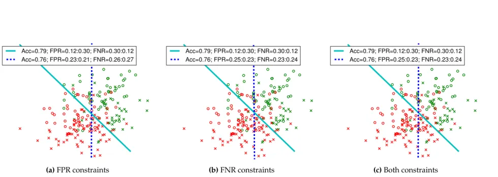
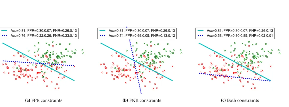
4.3 [Synthetic data with disparity in false positive as well as false neg-ative rates:DMF P R andDMF N Rhave opposite signs. Removing disparate mistreatment on FPR can potentially help remove dis-parate mistreatment on FNR. Removing disdis-parate mistreatment

on both at the same time leads to very similar results. . . 53

disparate mistreatment on FPR can potentially increase disparate mistreatment on FNR. Removing disparate mistreatment on both

at the same time causes a larger drop in accuracy. . . 54

5.1 A fictitious decision making scenario involving two groups: men (M) and women (W). Featuref1 (x-axis) is highly predictive for women whereasf2 (y-axis) is highly predictive for men. Green (red) quadrants denote the positive (negative) class. Within each quadrant, the points are distributed uniformly and the numbers in parenthesis denote the number of subjects in that quadrant. The left panel shows the optimal classifier satisfying parity in treatment. This classifier leads to all the men getting classified as negative. Themiddle panelshows the optimal classifier satis-fying parity in impact (in addition to parity in treatment). This classifier achieves impact parity by misclassifying women from positive class into negative class, and in the process, incurs a signif-icant cost in terms of accuracy. Theright panelshows a classifier consisting of group-conditional classifiers for men (purple) and women (blue). Both the classifiers satisfy the preferred treatment criterion since for each group, adopting the other group’s classifier would lead to a smaller fraction of beneficial outcomes (refer to Section5.1for a discussion on group- vs. individual-level pref-erences). Additionally, this group-conditional classifier is also a preferred impact classifier since both groups get more benefit as compared to the impact parity classifier. The overall accuracy is

better than the parity classifiers. . . 63

variant of the one in Figure5.1, with the difference being that the (positive and negative) classes are not perfectly separable in this case (even with group-conditional classifiers). On this dataset,

30%of the men receive beneficial outcomes with their own clas-sifier whereas10%receive beneficial outcomes with the classifier of women. So the preferred treatment criterion (for group-level preferences) is satisfied, as men would prefer their own classi-fier as a group. However, some of the men who did not receive beneficial outcomes under their own classifier, receive beneficial outcomes when using the classifier of women,i.e., the men inside the bottom left (red) quadrant who are on the right side of the classifier for women (blue line). So these men would individu-allyprefer women’s classifier, even though the men’s group as a whole prefers their own classifier. Hence, while this setup pro-vides preferred treatment for men at a group-level, it does not provide preferred treatment at an individual-level. (For women, the setup provides preferred treatment both at a group as well as

at an individual-level.) . . . 68

5.3 [Linearly separable synthetic data] Crosses denote group-0 (points withz = 0) and circles denote group-1. Green points belong to the positive class in the training data whereas red points belong to the negative class. Each panel shows the accuracy of the decision mak-ing scenario along with group benefits (B0 andB1) provided by each of the classifiers involved. For group-conditional classifiers, cyan (blue) line denotes the decision boundary for the classifier of group-0 (group-1). Parity case (panel (b)) consists of just one classifier for both groups in order to meet the treatment parity criterion. Preference-based measures can significantly lower the

cost of nondiscrimination. . . 73

5.4 [Non- linearly-separable synthetic data] Crosses denote group-0 (points with z = 0) and circles denote group-1. Green points belong to the positive class in the training data whereas red points belong to the negative class. Each panel shows the classifiers with top row containing the classifiers for group-0 and the bottom for group-1, along with the overall accuracy as well as the group benefits (B0 andB1) provided by each of the classifiers involved. For parity classifier, no group-conditional classifiers are allowed,

so both top and bottom row contain the same classifier. . . 74

‘Prf-treat.’, ‘Prf-imp.’, and ‘Prf-both’ respectively correspond to the classifiers satisfying preferred treatment, preferred impact, and both preferred treatment and impact criteria. Sensitive feature values0and1denote blacks and whites in ProPublica COMPAS dataset and NYPD SQF datasets, and women and men in the Adult dataset. Bi(θj)denotes the benefits obtained by group i when using the classifier of groupj. For theParitycase, we train just one classifier for both the groups, so the benefits do not change

by adopting other group’s classifier. . . 75

4.1 In addition to the overall misclassification rate, error rates can be measured in two different ways: false negative rate and false positive rate are defined as fractions over theclass distribution in the ground truth labels, or true labels. On the other hand, false discovery rate and false omission rate are defined as fractions over

theclass distribution in the predicted labels. . . 44

4.2 Performance of different methods while removing disparate mis-treatment with respect to false positive rate, false negative rate and both. When provided with the same amount of information, our technique as well as the post-processing technique of Hardt et al. lead to similar accuracy for the same level of disparate

mistreatment. The baseline tends to present the worst results. . . 59

6.1 Capabilities of different methods in eliminating disparate treat-ment (DT), disparate impact (DI) and disparate mistreattreat-ment (DM). We also show the type of each method: pre-processing (pre), in-processing (in) and post-processing (post). None of the prior methods addresses disparate impact’s business necessity (BN) clause. Many of the methods do not generalize to multiple (e.g., gender and race) or polyvalent sensitive features (e.g., race, that has more than two values). The strategy by (Feldman et al.,

2015) is limited to only numerical non-sensitive features. . . 81

6.2 A broad overview of different notions of fairness /

nondiscrimina-tion in the machine learning literature. . . 85

A.1 [Adult dataset] Class distribution for different genders. The classes

are: whether a person earns more than50K USD per year or not. . . 97

A.2 [Adult dataset] Class distribution for different races. The classes

are: whether a person earns more than50K USD per year or not. . . 97

A.4 [ProPublica COMPAS dataset] Class distribution for different races. The classes are: whether a defendant would receidivate

within two years or not. . . 98

A.5 [NYPD SQF dataset—original] Class distribution for different races. The classes are: whether or not an illegal weapon would be

recovered on a pedestrian stopped at the suspicion of carrying one. . . 98

A.6 [NYPD SQF dataset—with balanced classes] Class distribution for different races. The classes are: whether or not an illegal weapon would be recovered on a pedestrian stopped at the suspicion of

carrying one. . . 98

C

HAPTER

1

Introduction

1.1

Algorithmic decision making in social domains

Data-driven algorithmic decision making has been used in applications involving hu-man subjects for several decades. For instance, credit scoring algorithms were being deployed in practice in as early as the 1950s (FICO,2018a;Furletti,2002), and parole risk assessment algorithms have been in use since the 1970s (Hoffman and Beck,1974;

Kehl and Kessler,2017). However, with the advent of complex learning methods, and convenient accessibility of “big data”, algorithmic decision making is permeating into an ever-increasing number of human-centric applications, where algorithms are used to assist, or sometimes even replace human decision makers. Some examples include job screening (Posse,2016), healthcare (Bhardwaj et al.,2017), community safety (Perry,

2013), product personalization (Covington et al.,2016), online ad delivery (Graepel et al.,

2010) and social benefits assignments (Niklas et al.,2015).

Algorithmic decision making has shown great promise in increasing the accuracy and scalability of the applications under consideration. For example, a recent study byLiu et al.(2017) shows that machine learning models can achieve a performance com-parable to that of humans when detecting cancer metastases. Goel et al.(2016) show that in applications such as stop-question-and-frisk (Meares,2014)—where pedestrians are stopped by police officers on the suspicion of possessing illegal weapons—algorithmic decision making can recover the majority of illegal weapons, while making much fewer stops (6%) as compared to human decision makers (that is, the police officers). Similarly,

Kleinberg et al.(2018) found that when making bail decisions, algorithms can signif-icantly reduce the crime rate (by 25%) while maintaining the same incarceration rate. Several other studies have also shown evidence that algorithms can help increase the performance of the task at hand in domains ranging from hiring (Kuncel et al.,2013,

Algorithmic decision making also presents potential for several additional advan-tages, such as, reducing the arbitrariness and implicit human biases in decision making. For example, while different human judges are known to grant different decisions to similar defendants (Dobbie et al.,2018;Kleinberg et al.,2018), algorithms can be easily designed to overcome this issue. Similarly, whereas human judgments can be poten-tially swayed (unintentionally) by various factors ranging from unconscious human biases (Badger,2016;Tatum,2017) to the hunger level of human judges (Danziger et al.,

2011), the design of algorithmic decision making systems suggests that they can trivially avoid these problems.

1.2

Discrimination in algorithmic decision making systems

Despite its apparent advantages, algorithmic decision making has also caused concerns about potential discrimination against people with certain social traits (e.g., gender, race), also referred to assensitive features.

For example, Sweeney(2013) found that Google’s AdSense platform was dispropor-tionately associating predominantly African-American names as having arrest records, as compared to the predominantly White names. A recent analysis by ProPublica claimed that COMPAS, a recidivism risk assessment tool used in courts across several locations in the United States (US), was biased against African-American defendants (Angwin et al.,

2016). An analysis byBolukbasi et al.(2016) revealed that theword2vec word embed-dings (Mikolov et al.,2013) used in a number of downstream tasks such as translation, web search and sentiment analysis, were biased along gender stereotypes present in the society. Similarly, a number of other instance have been reported where algorithms (unintentionally) discriminated against certain social groups (Buolamwini and Gebru,

2018;Fussell,2017;Pachal,2015).

In this context, there have been calls from governments (Muñoz et al.,2016;Podesta et al.,2014), regulatory authorities (FTC,2016;Goodman and Flaxman,2016), civil rights unions (Eidelman,2017) and researchers (Barocas and Selbst,2016;O ´Neil,2016;Pasquale,

2015) to tackle the potential discriminatory effects of algorithmic decision making. For example, a recent report by the US Federal Trade Commission (FTC,2016) points out that data-driven algorithmic decision making can “create or reinforce existing disparities” or “create new justification for exclusion”, and urged that “companies should assess the factors that go into an analytics model and balance the predictive value of the model with fairness considerations”. Similarly, Recital 71 of the European General Data Protection Regulation (GDPR) that came into effect in May 2018, requires organizations handling personal data of European Union (EU) users to “prevent, inter alia, discriminatory effects

on natural persons on the basis of” certain social traits such as sexual orientation and ethnic origin (Goodman and Flaxman,2016;Goodman,2016).

1.3

Challenges in tackling discrimination

While avoiding discrimination based on certain socially salient traits (e.g., gender, race) is a legalprinciplein many countries (Altman,2016;Civil Rights Act,1964), eliminating discrimination from algorithmic decision outcomes poses a tough challenge. Two of the major reasons for this difficulty are:

I. Algorithmic decision making systems are typically designed to optimize for pre-diction accuracy while enabling efficient training. Efficient training here refers to finding the optimal algorithm parameters rapidly, and is a crucial property while learning from large training datasets (Bishop,2006). Incorporating nondiscrimina-tionmechanismsinto these systems—i.e., optimizing for prediction accuracyunder

nondiscrimination constraints—while simultaneously preserving efficient training, is often quite difficult.

II. While the nondiscrimination principle “enjoys impressive global consensus” ( Alt-man,2016), operationalizing this principle tomeasurediscrimination (to eventually eliminate it) is a non-trivial task. Here, operationalization refers to the process of formalizing orinterpretinga fuzzy concept so as to make itmeasurablefor empirical observations (Lukyanenko et al.,2014). For example, what constitutes a discrimina-tory practice in one case might not do so in another. In fact, one widely accepted measure of discrimination (namely, disparate impact), is known to lead to “reverse discrimination” if applied out of context (Ricci,2009).

1.4

Thesis contributions

This thesis tries to address the above challenges. Below, we discuss our research contri-butions towards this end.

I. Proposing mechanisms for existing nondiscrimination measures

Existing studies in discrimination-aware machine learning mostly quantify discrimina-tion using two measures inspired by anti-discriminadiscrimina-tion legisladiscrimina-tion in various countries: disparate treatment anddisparate impact (Barocas and Selbst,2016). As we will dis-cuss in detail in Section2, while it is desirable to train decision making systems that

are nondiscriminatory with respect to both the measures, doing so in practice is quite difficult due to computational complexities involved.

To overcome the computational issues in training nondiscriminatory classifiers, we propose a novel and intuitive mechanism of decision boundary covariance. This mechanism satisfies several desirable properties: (i) it can limit discrimination with respect to both disparate treatment and disparate impact; (ii) for a wide variety of convex boundary-based linear and non-linear classifiers (e.g., logistic regression, SVM), it is convex and can be readily incorporated in their formulation without increasing their complexity, hence ensuring efficient learning; (iii) it allows for clear mechanisms to trade-off nondiscrimination and accuracy; and, (iv) it can be used to ensure nondiscrimination with respect to several sensitive features.

Experiments using both synthetic and real-world data show that our mechanism allows for a fine-grained control of the level of nondiscrimination, often at a small cost in terms of accuracy, and provides more flexibility than the state-of-the-art.

II. Proposing new measures of nondiscrimination (and designing mechanisms)

We also propose new measures of nondiscrimination that can avoid some shortcomings of the existing measures.

First, we argue that while the disparate impact measure of nondiscrimination might be quite intuitive in certain situations—e.g., situations where the historical decisions in the training data are potentially biased (i.e., groups of people with certain sensitive attributes may have historically received discriminatory treatment), its utility is somewhat limited in cases when the ground truth training labels are available. We then propose an alternative measure of nondiscrimination, disparate mistreatment, which is useful in situations when the validity of historical decisions in the training data can be ascertained.

Next, we note that while existing measures of nondiscrimination in machine learning are based on parity (of treatment or impact), under some interpretations, a lack of parity might not necessarily constitute as discrimination. Specifically, drawing inspiration from the concepts of fair-divisions and envy-freeness in economics and game theory, we pro-pose two additional measures of nondiscrimination: preferred treatmentandpreferred impact. These measures are useful in situations when feature and class distributions of different groups subject to the decision making are significantly different. These measures are based on the idea that certain distributions of outcomes might be preferred by different groups even when the outcomes do not necessarily follow parity as specified by disparate treatment and disparate impact. We also show that these new measures can help reduce the cost of nondiscrimination.

We also extend our decision boundary covariance mechanism and incorporate the newly proposed nondiscrimination measures into the formulations of convex boundary-based classifiers, this time as convex-concave constraints. The resulting formulations can be solved efficiently using recent advances in convex-concave programming.

1.5

Thesis outline

The rest of this thesis is organized as follows:

• In Chapter 2, we provide background on discrimination in machine learning. Specifically, we discuss the concept of discrimination in the context of social sciences and law. We then describe how discrimination is measured in classification tasks. • In Chapter3, we design mechanisms to eliminate discrimination from classification outcomes, when it is measured using existing notions of disparate treatment and disparate impact.

• In Chapter4, we propose a new measure of discrimination which we refer to as disparate mistreatment. We describe how disparate mistreatment can overcome some shortcomings of the existing measure of disparate impact. We also propose mechanisms to train classifiers without disparate mistreatment.

• In Chapter5, we depart from the legal perspective of discrimination and introduce two new measures of discrimination: preferred treatment and preferred impact, which are inspired by ideas from economics and game theory. We then design mechanisms to train classifiers satisfying these two new (non)discrimination crite-ria.

• In Chapter 6, we review literature from various areas related to discrimination-aware algorithmic decision making.

• In Chapter 7, we add a discussion on the limitations of our work, and explore avenues of future work.

C

HAPTER

2

Background

In this chapter, we provide background on important concepts used throughout this thesis. We start off by discussing the concept of discrimination. Next, considering that most existing notions of discrimination in machine learning literature are inspired by anti-discrimination laws, we describe different measures used to detect discrimination in legal domains in various countries. We then close the chapter by explaining how these measures are formalized in the area of machine learning.

2.1

What is discrimination?

After reviewing literature from various domains including law and philosophy,Altman

(2016) defines discrimination as practices that:1

“wrongfully impose a relative disadvantage on persons based on their membership in a salient social group”

While the definition is quite intuitive at the first glance, there are several important points to be considered:

Discrimination is a relative phenomenon. Altman notes that discrimination occurs when a person or a group is given disadvantageous treatmentrelative tosome other group. He notes that this point is affirmed by the US Supreme Court case,Brown v. Board of Education (Brown,1954) which ruled that racial segregation in public schools was discriminatory because it put African-Americans children at arelativedisadvantage as compared to White children.

Moreover,Altmancontrastsdifferential treatmentwithrelative disadvantage, and men-tions that not all groups that receive different treatment from each other are being

discriminated against. He argues that under the segregation practices in the Ameri-can South, while the treatment of AfriAmeri-can-AmeriAmeri-cans and Whites was different from each other, and while this differential treatment might have held back the progress for everyone in the South, only African-Americans (and not Whites) were the victims of discrimination.

Not all groups are socially salient. While society can be divided into groups along different dimensions (e.g., based on eye color, music preferences), not all ways of group-ing people form salient social groups. Accordgroup-ing toLippert-Rasmussen(2006), socially salient groups are the ones that are “important to the structure of social interactions across a wide range of social contexts”.

On a more legal side, salient social groups (also called protected groups),2_among

other factors, are formed based on groupings that were the basis of consistent social injustices and oppression in the past (Altman,2016;Barocas and Hardt,2017). As a result, laws in different countries define socially salient groups accordingly. For example, with respect to employment, the protected features under the US anti-discrimination law are: race, color, gender, religion, national origin, citizenship, age, pregnancy, familial status, disability status, veteran status and genetic information (Barocas and Hardt,2017). EU law has a very similar list of protected grounds. Interestingly, EU law also designates language as a protected ground (Fribergh and Kjaerum,2010).

Finally, based on the contemporary discourse in a society, the definition of salient social groups is subject to change (Zarsky,2014). For example, under US law, genetic information was only designated as a protected feature3_{in 2008 (Green et al.,2015).}

Not all domains are regulated. Not all application domains in a society are regulated by anti-discrimination laws. For example, under the US law, the regulated domains are credit, education, employment, housing, public accommodation and marketing (Barocas and Hardt,2017). Furthermore, the designation of protected groups may also vary across various domains. For example, under the US anti-discrimination law, health insurers

2_{While legal literature refers to salient social groups as “protected groups” (Barocas and Selbst,2016),}

some studies in machine learning literature also refer to them as “sensitive feature groups” (Pedreschi et al.,2008). Thus, we will be using the termssalient social group,protected groupandsensitive feature group interchangeably.

3_{We refer to the features or traits that form the basis of protected groups (e.g., the feature race forms the}

groups: African-American, Hispanic, ...) associally salient group memberships,protected featuresorsensitive features.

are prohibited from discriminating based on genetic information, but no such provision exists with respect to gender, race or religion (Avraham et al.,2014;GINA,2008).

Discrimination involves groups. A point worth mentioning at this stage is that the phenomenon of discrimination by definition involves having discernible groups. For example, an employer putting applicants at relative disadvantage arbitrarily (without regard to their salient social group membership) might be unfair to the applicants in question, but (s)he will not be committing discrimination. Such scenarios involving

individual-level fairness have previously been considered in moral philosophy (Rawls,

2009) as well as in machine learning (Dwork et al.,2012;Joseph et al.,2016;Speicher et al., 2018). On a high-level, these individual-level fairness notions require that all individuals at the same level of qualification (regardless of their group membership) should be treated similarly.

The wrongs of arbitrary rejections vs. the discriminatory rejections (based on salient social groups) are different. According toArneson (2015): “Whereas being the object of discrimination because one belongs to a group that has been targeted for oppressive treatment in the past is likely to be a wound to one’s sense of dignity and self-respect, being the victim of whimsical or idiosyncratic hiring practices is less likely to inflict a significant psychic wound over and above the loss of the job itself. Also, since whimsical discrimination is idiosyncratic, it will not lead to cumulative harm by causing anyone to be the object of economic discrimination time after time (unless whimsical hiring were common and one were extremely unlucky)”.

For further discussion into the concept of discrimination (and related ideas), we point the interested reader toAltman(2016) andArneson(2015) and references therein.

2.2

Measures of discrimination in legal domains

Having analyzed the definition of discrimination in Section2.1, the question that arises now is, how does one operationalize this definition? That is, how does one empirically

measureif a (algorithmic) decision making system is discriminatory? Recall from Sec-tion2.1that in measuring discrimination, our aim is to see if a decision making system imposeswrongful relative disadvantageon certain socially salient groups.

Since much of the work in discrimination-aware machine learning until now has been inspired by anti-discrimination legislation, we now briefly survey how discrimination is measured in various legal systems. Specifically, our goal will be to understand how anti-discrimination laws interpret wrongful relative disadvantage in the definition of discrimination in Section2.1.

For the sake of conciseness, we will mostly focus on anti-discrimination legislation from the US and the EU. Our terminology will be driven by the US anti-discrimination laws, and we will mention the terminology used in the EU law whenever significant differences arise. For a more detailed account into the discussion that follows, we point the reader to (Altman,2016;Bagenstos,2015; Barocas and Selbst,2016;FDIC’s Compliance Examination Manual,2017;Fribergh and Kjaerum,2010;Gano,2017;Romei and Ruggieri,2014;Siegel,2014).

Anti-discrimination laws mostly differentiate between two distinct forms of discrim-ination: disparate treatmentanddisparate impact.

2.2.1

Disparate treatment

This measure is referred to as “direct discrimination” under the EU law (Fribergh and Kjaerum,2010).

What constitutes disparate treatment?

According Title VII of the US Civil Rights Act of 1964, a decision making process suffers from disparate treatment if it: (i) explicitly or formally considers the sensitive group membership of a person in question, or (ii) it bases the decisions on some other factors with theintent to discriminateagainst certain groups (Barocas and Selbst,2016). EU law also defines disparate treatment in a similar way (Fribergh and Kjaerum,2010).

The specification above raises the following interesting points.

Once a decision maker explicitly considers the protected ground (e.g., gender) in making the decision, even if the protected group membership has minimal impact on the decisions—perhaps because other (non-protected) features carried higher weight—this would still count as disparate treatment (Barocas and Selbst,2016).

Also, a decision maker could implicitly base the decisions on sensitive features. For example, under the redlining practice in the US, a lender would deny credit to residence of certain neighborhoods based on the racial makeup of that neighborhood (Barocas and Selbst,2016;Gano,2017). This case would also count as disparate treatment since the lender’s decision to not issue credit is based on racial profiling of the neighborhood rather than considering the merits of individuals living in that neighborhood. According toBarocas and Selbst(2016): “Redlining is illegal because it can systematically discount entire areas composed primarily of members of a protected class, despite the presence of some qualified candidates.”

Finally, under certain circumstances, it may be permissible to base decisions on the protected group membership information.

For example, under Title VII of the US Civil Rights Act of 1964, an employer can justify using the protected group membership information when it qualifies as a “Bona fide occupational qualification” (BFOQ) for the job under consideration (Berman,2000). A sensitive feature can be considered a BFOQ when it is “reasonably necessary to the normal operation of that particular business”. For example, due to safety reasons, mandatory retirement ages can be enforced on airline pilots or air traffic controllers since age is a BFOQ for these jobs (Altman,2016).

Similarly, use of sensitive features in decision making could be permitted when the goal is to advance a compelling governmental interest (e.g., affirmative action policies aimed at improving racial diversity in colleges). However, asMacCarthy(2017) notes, such scenarios (where sensitive features such as race are explicitly used in decision making) would likely be subject to strict judicial scrutiny by the courts, and would need to satisfy certain stringent criteria to pass the strict scrutiny test.

How is disparate treatment detected?

We briefly discuss how disparate treatment is detected in the legal domain, since this discussion would be useful in the later part of the thesis (Sections2.4and Chapter7). In the discussion that follows, theplaintiff refers to the party that lodges a discrimination complaint before a court (e.g., a potential employee who was rejected) and thedefendant

refers to the party against whom the case is lodged (e.g., the employer). A disparate treatment liability can be established in two different ways:

The first method is where the plaintiff can showdirect evidencethat the protected group membership was a motivating factor in the defendant’s decision, e.g., a bar advertising publicly that they do not serve certain minorities (Altman,2016).

The plaintiff can showindirect evidenceof discrimination. Under US legal system, this is done viaMcDonnell-Douglas burden-shifting schemeorPrice-Waterhouse mixed motive regime (Barocas and Selbst, 2016; Gano, 2017), whereas under EU law, a comparator

framework is used (Fribergh and Kjaerum,2010). Roughly, this method requires the plaintiff to show that the action to reject the plaintiff could not have been taken had the defendant not taken the sensitive group membership into account,i.e., the plaintiff would not have received the negative outcome had their sensitive group membership been different (e.g., had she been White and not African-American).

Finally, under the US anti-discrimination doctrine, while many sources argue that disparate treatment always corresponds to intentional discrimination—i.e., the decision maker knowingly basing decisions on the protected group membership of a person (either directly, or via a proxy) (Federal Reserve,2016;Gano,2017;Gold,2004)—others

argue that disparate treatment may very well stem unintentionally,e.g., from unconscious biases (Barocas and Selbst,2016;Krieger and Fiske,2006). However, asBarocas and Selbst

(2016) note, “the law does not adequately address unconscious disparate treatment”, and it is not entirely clear how such cases would be addressed.4 On the other hand, the EU law does not require the presence of intent in order to establish a disparate treatment liability (Fribergh and Kjaerum,2010;Maliszewska-Nienartowicz,2014).

2.2.2

Disparate impact

This measure is referred to as “indirect discrimination” under the EU law (Fribergh and Kjaerum,2010).

What constitutes disparate impact?

Under both US and EU laws, disparate impact occurs when “facially neutral” decision making (e.g., a hiring exam) results in disproportionately adverse impact on a certain protected group (Barocas and Selbst,2016).

Adverse impact here is said to occur when the success rates for persons from dif-ferent groups (e.g., African-Americans vs. Whites) are substantially different. How different is “substantially different” is often determined on a case-by-case basis in the EU law (Fribergh and Kjaerum,2010). The same holds true for the US justice system. However, as a rough guideline in the hiring domain, the US Equal Employment Oppor-tunity Commission suggests having an impact ratio between the two groups to be no less than80%(Biddle,2005). As an example, a scenario where50%of White applicants get hired, whereas only10%of African-American applicants get accepted, the impact ratio is 10

50 = 0.2.

It is vital to note that disproportionally adverse impact does not automatically constitute a disparate impact liability. Both US and EU legislations accommodate a business necessity defense that can justify the adverse impact. For more details regarding this justification, we next describe how a disparate impact liability is established.

How is disparate impact detected?

Under the US judicial system, the process of establishing a disparate impact liability proceeds as follows (Barocas and Selbst,2016): (i) The plaintiff shows that a facially neutral decision making process (e.g., a hiring exam) led to disproportionate adverse

4_{As we discuss shortly in Section2.2.2, some authors argue that the disparate impact doctrine might be}

impact on the protected group. (ii) The defendant can then show that the decision making process is related to the job and is a “business necessity”,i.e., the adverse impact is unavoidable. (iii) The plaintiff can counter by demonstrating that the defendant could have used an alternative decision making regime that would achieve the same outcome utility for the defendant while having lesser adverse impact. EU courts allow a similar business necessity defense (Fribergh and Kjaerum,2010).

For example, in the US Supreme Court caseGriggs vs. Duke Power Co.(Griggs,1971), the court was able to establish that the hiring criteria of Duke Power Co. was not job-related, hence the adverse impact on African-Americans constituted a case of disparate impact. On the other hand, inRicci vs. DeStefano(Ricci,2009), the court foundno evidence

that the promotion test used by the New Haven Fire Department was not related to the job and hence ruled that there would be no disparate impact liability.

The justification behind disparate impact as a discrimination measure

Disparate impact is known to be a highly controversial notion of discrimination with some arguing about its validity as a suitable discrimination measure (Altman,2016;

Barocas and Selbst,2016).

However,Siegel(2014) notes that disparate impact can be useful as a discrimination measure when one aims to either root outwell-hidden disparate treatment(e.g., an employer using proxies to intentionally discriminate against protected groups) or to address

unconscious and structural discrimination that can arise as a result of historical biases. Specifically, she gives the following reasons about the effectiveness of disparate impact as measure of discrimination.

“Why impose disparate impact liability? Judges and commentators, both liberal and conservative, understand disparate impact liability to redress at least three kinds of discrimination that are common in societies that have recently repudiated centuries old traditions of discrimination.

The first is covertintentional discrimination[emphasis added]. Once a soci-ety adopts laws prohibiting discrimination, discrimination may simply go underground. When discrimination is hidden, it is hard to prove. Disparate impact tests probe facially neutral practices to ensure their enforcement does not mask covert intentional discrimination.

The second isimplicit or unconscious bias[emphasis added]. Discrimination does not end suddenly; it fades slowly. Even after a society repudiates a system of formal hierarchy, social scientists have shown that traditional

norms continue to shape judgments in ways that may not be perceptible even to the decision maker herself. Disparate impact tests probe facially neutral practices to ensure their enforcement does not reflect implicit bias or unconscious discrimination.

The third form of bias is sometimes termedstructural discrimination[emphasis added]. An employer acting without bias may adopt a standard that has a disparate impact on groups because the standard selects for traits whose allocation has been shaped by past discrimination, whether practiced by the employer or by others with whom the employer is in close dealings. Disparate impact tests probe facially neutral practices to ensure their enforcement does not unnecessarily perpetuate the effects of past intentional discrimination.” Regardless, disparate impact remains a contentious measure, and its applicability is assessed on a case-to-case basis—see for exampleGriggs vs. Duke Power Co.(Griggs,1971),

Ricci vs. DeStefano(Ricci,2009),Texas Department of Housing and Community Affairs vs. Inclusive Communities Project, Inc.(Inclusive Communities,2015) andFisher vs. University of Texas(Fisher,2016).

In this thesis, when discussing disparate impact, we will assume that the adminis-trator of the decision making system aims at removingsubstantial differencesbetween the beneficial outcome rates for different groups. That is, given a decision making system where the beneficial outcome rates are different for different groups, the admin-istrator might be interested in accessing an array of decision making outcomes, with decreasing values of disparity in beneficial outcome rates (e.g., where the disparity in beneficial outcome rates is 0.5, 0.4,. . ., 0.0). However, as described above, a disparity in decision outcomes does not always generate a disparate impact liability for the system administrator—in the case of a legitimate business necessity, the system administrator could still justify the disparity.

Finally, somewhat related with the disparate impact doctrine is the notion of affir-mative action (Barocas and Selbst,2016; MacCarthy, 2017; Siegel,2014). The goal of affirmative action is often to correct for historical discrimination against certain groups. Affirmative action may involve (among other things) giving preferential treatment to these groups (e.g., by setting up quotas, giving special treatment to these groups). How-ever, affirmative action is allowed under very special circumstances and is known to be highly controversial (Fribergh and Kjaerum,2010;Fullinwider,2018).

2.2.3

How do disparate treatment and disparate impact capture

wrong-ful relative disadvantage?

The reasons for interpreting disparate treatment and disparate impact to be causing wrongful relative disadvantage are plentiful. Here, we describe a few of these reasons. A detailed discussion on them can be found in (Altman,2016).

A decision making process incurring disparate treatment (i.e., intentionally basing decisions on sensitive feature information) can be interpreted as causing wrongful relative disadvantage since it judges people based on immutable traits that they do not have any control over (e.g., race, national origin), and it may cause arbitrary and inaccurate stereotyping that is not relevant to the task at hand.

Similar arguments hold for disparate impact, with the addition that disparate im-pact also tries to capture implicit biases in the decision making process, as well as the structural discrimination where the biased historical treatment of certain groups results in these groups consistently getting disadvantageous outcomes in the present.

We now move on to the design of algorithmic decision making systems, and see how disparate treatment and disparate impact are measured in the context of algorithmic decision making.

2.3

Setup of a binary classification task

In this thesis, we focus on a specific (supervised) learning task: classification. Moreover, we only consider binary classification tasks. The reason is as follows: discrimination analysis often involves tasks where the outcomes are binary in nature, with a clear distinction between a desirable (e.g., getting accepted for a job) and an undesirable (e.g., getting rejected from a job) outcome. However, the techniques proposed in the later sections can be extended to m-ary classification tasks as well.

In a binary classification task, given a training set,D =_{(xi, yi)}Ni=1, consisting ofN users, one aims at learning a mapping between user feature vectorsx_∈Rdand the class labels y∈ {−1,1_}. Here, one assumes that(x, y)are drawn from an unknown feature distributionf(x, y).

Learning this mapping can be done using various methods. In this thesis, we focus on a broad class of learning methods: convex decision boundary-based classifiers such as logistic regression, linear and non-linear support vector machines (SVMs),etc.

Under convex boundary-based classifiers, the learning reduces to finding a decision boundary defined by a set of parametersθin the feature space that separates the users in the training set according to their class labels. One typically looks for a decision

boundary, denoted asθ∗, that minimizes a certain loss functionL(θ)over the training set,i.e.,θ∗ = argmin_θL(θ). For convex boundary-based classifiers,Lis a convex function of the decision boundary parametersθ, meaning that the globally optimal solution,θ∗, can be foundefficientlyeven for large datasets.

Then, for a given unseen feature vector x, one predicts the class label yˆ = 1 if

dθ∗(x)≥0, andyˆ= 1otherwise. Here,d_θ∗(x)denotes the signed distance fromxto the decision boundary,θ∗.

We now give examples of some well-known convex boundary-based classifiers:

Logistic regression. In logistic regression (and other linear convex boundary-based classifiers), the distance from decision boundary is denoted asdθ(x) = θTx. In other words, the decision boundary is represented by the hyperplaneθT_{x= 0, since we predict}

ˆ

y= 1ifdθ(x)≥0andyˆ= 1 ifdθ(x)<0.

Next, in logistic regression, one maps the feature vectorsxto the class labelsyby means of a probability distribution:

p(y= 1_|x,θ) = 1

1 +e−dθ(x) =

1

1 +e−θT_x, (2.1)

It is easy to see that a point lyingat the decision boundary, i.e., with dθ(x) = 0, has

p(y = 1_|x,θ) = 0.5, and this probability increases with an increase in the (signed) distance from the boundary.

One obtains the optimal value ofθ by solving the following maximum likelihood problem over the training set (Murphy,2012):

minimize

θ −

X

(x,y)∈D

logp(y_|x,θ). (2.2)

Linear SVM.In the case of a linear SVM, the optimal decision boundary corresponds to the maximum margin decision hyperplane (Bishop,2006). This boundary is found by solving the following optimization problem:

minimize θ kθk 2_+CPN i=1ξi subject to yiθTxi ≥1−ξi,∀i∈ {1, . . . , N} ξi ≥0,∀i∈ {1, . . . , N}, (2.3)

whereθandξare the variables. Here, minimizingkθ_k2 _{corresponds to maximizing the} margin between thesupport vectorsassigned to the two classes, andCPn

i=1ξipenalizes the number of data points falling inside the margin.

Nonlinear SVM. In a nonlinear SVM, the decision boundary is represented by the hyperplane θTΦ(x) = 0, where Φ(_·) is a nonlinear transformation that maps every feature vectorx into a higher dimensional transformed feature space. Similar to the case of a linear SVM, one may think of finding the parameter vector θ by solving a constrained quadratic program. However, the dimensionality of the transformed feature space can be large, or even infinite, making the corresponding optimization problem difficult to solve. Fortunately, we can leverage the kernel trick (Schölkopf and Smola,

2002) and resort instead to the dual form of the problem, which can be solved efficiently. In particular, the dual form is given by (for conciseness, we use the dual form notation ofGentle et al.(2012)):

minimize α 1 2α T_Gα−1T_α subject to 0_≤α_≤C, yT_{α= 0,} (2.4)

where α = [α1, α2, . . . , αN]T are the dual variables, y = [y1, y2, . . . , yN]T are the class labels, Gis the N _×N Gram matrix withGi,j =yiyjk(xi,xj), and the kernel function k(xi,xj) = hφ(xi), φ(xj)idenotes the inner product between a pair of transformed fea-ture vectors. The distance from decision boundary is computed as: dα(x) =

PN

i=1αiyik(x,xi). Finally, the optimization problems above can be altered easily to accommodate cases where one wants to assign different cost to different type of errors,e.g., assigning different cost to false positives and false negatives (Bishop,2006).

2.4

Disparate treatment and disparate impact in binary

classification

Continuing from the setup of a binary classifier in Section2.3, we also assume that each user feature vectorxin the datasetDis accompanied by a sensitive featurez _{∈ {}0,1_}.5 The sensitive feature is also drawn from an unknown distributionf(z)and it may be

5_{Recall from Section2.1that we use sensitive feature, protected feature and socially salient group}

dependent on the non-sensitive feature vectors x and class labelsy, i.e., f(x, y, z) =

f(x, y_|z)f(z)₆=f(x, y)f(z).

Notice that (i) we defined only one sensitive feature, and (ii) defined it to be binary. This is merely for the sake of exposition. In the later sections, we will provide examples of polyvalent and several sensitive features wherever necessary.

With this specification, we can formally describe the absence of disparate treatment and disparate treatment in the outcomes of a binary classification task.

No disparate impact.A binary classifier does not suffer from disparate impact if:

P(ˆy= 1_|z = 0) =P(ˆy= 1_|z = 1), (2.5)

i.e., if the probability that a classifier assigns a user to the positive classyˆ= 1is the same for both values of the sensitive featurez, then there is no disparate impact.

No disparate treatment. Assume that x_◦z represents the concatenation of the non-sensitive feature vectorxand the sensitive featurez. Also, with slight abuse of notation, we assume thatyˆ(x_◦z)represents the decision of a classifier for a user with the given non-sensitive and sensitive features.6 _{Then, a binary classifier does not suffer from}

disparate treatment if:

ˆ

y(xi◦0) = ˆy(xi◦1) ∀i∈ {1, . . . , N} (2.6) i.e., if the decision of the classifier does not change with a change in the user’s sensitive feature value, then there is no disparate treatment.

Relating our specification of disparate treatment in Eq. (2.6) to the definition of disparate treatment in Section2.2.1, we notice that Eq. (2.6) only accounts for scenarios when the sensitive feature is directlyused in the classification task. That is, Eq. (2.6) would not detect scenarios when a decision maker uses a proxy feature such as location

with the intentof discriminating against a certain sensitive feature group.

The difficulty with detecting such implicit disparate treatment via proxy variables is that in any classification task, most non-sensitive features (e.g., educational-level, location) will likely have non-zero correlation with the sensitive feature (e.g., gender). For example, a 2007 analysis of credit-based insurance scores by US Federal Trade Commission (FTC,2007) shows that a number of “informative” features are correlated

6_{For example, for convex boundary-based classifiers, yˆ(·) would be the sign of the distance from}

with race. Under such situations, it is very difficult to determine whether or not the decision maker had an intent to discriminate while using certain non-sensitive features.

To counter such scenarios, the disparate impact test (Eq.2.5) would be a more suitable tool to detect discrimination. In fact, asSiegel(2014) notes, one of the utilities of disparate impact tests is to detect “covert intentional discrimination” and “probe facially neutral practices to ensure their enforcement does not mask covert intentional discrimination”. Having formally described disparate treatment and disparate impact in the context of classification tasks, we now move on to design classifiers that can avoid these two forms of discrimination.

C

HAPTER

3

Classification without disparate

treatment and disparate impact

While it is desirable to design classifiers free of disparate treatment as well as disparate impact, controlling for both forms of discrimination simultaneously is challenging. One could avoid disparate treatment by ensuring that the decision making process does not have access to sensitive feature information (and hence cannot make use of it). However, ignoring the sensitive feature information may still lead to disparate impact in outcomes: since automated decision-making systems are often trained on historical data, if a group with a certain sensitive feature value was discriminated against in the past, this unfairness may persist in future predictions, leading to disparate impact (Barocas and Selbst,2016;Dwork et al.,2012). Similarly, avoiding disparate impact in outcomes by using sensitive feature information while making decisions would constitute disparate treatment, and may also lead to reverse discrimination (Ricci,2009).

In this chapter, our goal is to design classifiers—specifically, convex margin-based classifiers like logistic regression and support vector machines (SVMs)—that avoid

bothdisparate treatment and disparate impact, and can additionally accommodate the “business necessity” clause of disparate impact doctrine (Section2.2.2). According to the business necessity clause, an employer can justify a certain degree of disparate impact in order to meet certain performance-related constraints (Barocas and Selbst,

2016). However, the employer needs to ensure that the current decision making incurs theleast possibledisparate impact under the given constraints.

Since it is very challenging to directly incorporate the disparate impact requirement into the design of many well-known classifiers like logistic regression or SVM, we intro-duce a novel and intuitive mechanism of decision boundary covariance: the covariance between the sensitive features and the signed distance between the users’ feature vectors and the decision boundary of the classifier. The decision boundary covariance serves as a tractable proxy for measuring and limiting the disparate impact of a classifier.

Our covariance mechanism allows us to derive two complementary formulations for training nondiscriminatory classifiers: one that maximizes accuracy subject to nondis-crimination constraints, and enables compliance with disparate impact doctrine in its basic form (i.e., ensuring parity in beneficial outcomes for different sensitive feature groups); and another that minimizes discrimination subject to accuracy constraints, and can help fulfill the business necessity clause of disparate impact doctrine. Remarkably, both formulations can also avoid disparate treatment, since they do not use sensitive feature information while making decisions,i.e., their decisions satisfy Eq. (2.6).7 _Our

mechanism additionally satisfies several desirable properties: (i) for a wide variety of convex boundary-based linear and non-linear classifiers (e.g., logistic regression, SVM), it is convex and can be readily incorporated in their formulation without increasing their complexity, hence ensuring efficient learning; (ii) it allows for clear mechanisms to trade-off nondiscrimination and accuracy; and, (iii) it can be used to ensure nondis-crimination with respect to several sensitive features. Experiments using both synthetic and real-world data show that our mechanism allows for a fine-grained control of the level of nondiscrimination, often at a small cost in terms of accuracy, and provides more flexibility than the state-of-the-art.

Relevant publication

Results presented in this chapter are published in (Zafar et al.,2017b).

3.1

Methodology

First, to comply with the disparate treatment criterion in Eq. (2.6), we specify that the sensitive feature should not be a part of the decision making processi.e.,xandzconsist of disjoint feature sets.

Next, for training a classifier adhering to the disparate impact criterion in Eq. (2.5), one can add this criterion into the classifier formulation as follows:

minimize

θ L(θ)

subject to P(ˆy= 1_|z = 0)₋P(ˆy= 1_|z = 1)_≤, P(ˆy= 1_|z = 0)₋P(ˆy= 1_|z = 1)_{≥ −},

(3.1)

where a smaller value of∈R+would result in a classifier more adherent to Eq. (2.5). 7_{As we explain shortly in Section 3.1, the sensitive feature information is needed only during the}

Unfortunately, it is very challenging to solve the above optimization problem for convex boundary-based classifiers, since for many such classifiers (e.g., SVM) the proba-bilities are a non-convex function of the classifier parametersθand, therefore, would lead to non-convex formulations, which are difficult to solve efficiently. Secondly, as long as the user feature vectors lie on the same side of the decision boundary, the probabilities are invariant to changes in the decision boundary. In other words, the probabilities are functions having saddle points. The presence of saddle points furthers complicate the procedure for solving non-convex optimization problems (Dauphin et al.,2014).

To overcome these challenges, we next introduce a novel measure of decision bound-ary covariance which can be used as a proxy to efficiently design classifiers satisfying Eq. (2.5).

Our measure of decision boundary covariance stems from the intuition that if two groups have high disparity in their probabilities of being assigned to the positive class,

i.e., if Eq. (2.5) is far from being satisfied, then the average signed distances from decision boundary for the two groups are also likely to be quite different from each other. Hence, by controlling the relationship between the sensitive feature and the signed distance from decision boundary, one could hope to limit disparate impact in the predicted labels. We now formalize this intuition below.

3.1.1

Decision boundary covariance

Our measure of decision boundary covariance is defined as the covariance between the users’ sensitive feature,z, and the signed distance from the users’ feature vectors to the decision boundary,dθ(x),i.e.:

Cov(z, dθ(x)) =E[(z−z¯)(dθ(x