Vol. 7, No. 2, June 2019, pp.438-447 Available online at: http://pen.ius.edu.ba
Lung cancer classification using data mining and supervised learning
algorithms on multi-dimensional data set
Saadaldeen Rashid Ahmed Ahmed1, Israa Al_Barazanchi2, Ammar Mhana3 , Haider Rasheed Abdulshaheed4
1Information technology - Altinbas university, İstanbul 2,4
Baghdad College of Economic Sciences University, Baghdad
3 College of the Science -University of Baghdad
Article Info ABSTRACT
Received Jan 14th, 2019
These With recent developments in machine learning, data mining and computer vision, there is great potential for improvements in early detection of lung cancer using scans and data available. This paper details the methods and techniques used in our project, where the objective is to develop algorithms to determine whether a patient has or is likely to develop lung cancer using dataset images using data mining and machine learning for the classification and examination. We explore approaches to address the problem. Cancer is the most important cause of death globally. The disease diagnosis is a major process to treat the patients who are affected by cancer disease. The diagnosis process is more difficult comparatively known about the cancer disease detection. Developing a proposed data mining model is useful to diagnose the cancer disease once the cancer detection is accomplished using data mining for the examination and classification of machine learning supervised algorithms.
Keyword:
lung cancer detection, machine learning, data mining, classification.
Corresponding Author:
Saadaldeen rashid ahmed ahmed1 Information technology
Altinbas university
İstanbul, Turkey, https://orcid.org/0000-0003-2259-7437 [email protected].
1. Introduction
In this study, a proposed data mining model has been separated into two different techniques, but it performs consecutively. The techniques are classification and clustering method of conceptual modeling. Thus, the cancer data must be converted into a knowledge base which is called as training data. The cancer patient data and training data to be built with classification using decision tree. The classification and significant pattern analysis will generate the frequent patterns from the cancer dataset. The clustering techniques which analyze the frequent pattern mining cancer patient data to be cluster based on the type of cancer. The result in disease attribute from the frequent pattern mining can be highlighted as attribute disease impact in the clustering group is called as class variable. The way lung cancer is diagnosed is by inspecting a patient's scan images, looking for small blobs in the lungs called nodules. Finding a nodule is not in itself indicative of cancer; the nodules must have certain characteristics (shape, size, etc.) to support a cancer diagnosis.
Several approaches to address the detection and classification of lung nodules have been proposed in the literature, including both techniques that rely on traditional image processing and computer vision
tools, and those that rely on representation learning and data mining. Nodule detection generally relies on image segmentation techniques. Traditional image processing techniques make use of intensity and geometrical shape features of connected components, graph cuts and active contours [2], and fuzzy c-means clustering [1]. Recently, machine learning algorithms have shown to be good for segmenting neuronal structures and identifying regions with nodules. A distinctive feature of the network is that it combines low-level features at the early layers with sampled higher-level features at the layers to make its predictions. The approach is much faster than those in which a classifier is trained to predict each pixel based on the surrounding patch [3], since it does not require the network to make pixel-level predictions. Other approaches rely on information for detection, such as using a machine learning to classify sub-volumes as either containing a nodule or not or using a voxel-level classification approach with a machine learning algorithm [3]. For the classification of segmented nodules, reported methods have used an autoencoder-based approach with a binary decision tree [3], deep features extracted from algorithms and passed to SVM and k-nearest neighbor, the classifier, while earlier approaches relied on manually computed shape, texture, and size features of segmented nodules with shallow classifiers like LDA, quadratic discriminant and logistic regression. Therefore, computer processing to assist lung cancer detection is one of most timely need of the world. Here we proposed an intelligent system for binary classification problem to detect the presence of lung cancer in a given patient-CT-lung scan. The proposed system uses combination of machine learning, feature based machine learning and rule-based processing to assess whether a given scan and data is of cancerous patient or not. It will output top candidate regions for nodules, common shape and texture parameters for each nodule region-of-interest, malignancy estimation for each nodule region of interest and overall malignancy of the whole scan and data available. Such a system will dramatically reduce the false positive rate that plagues the current detection technology. And help to find nodules missed by human error [4]. Regardless of the malignancy outcome, automatic nodule detection can be a big help for radiologists since the nodules can easily be overlooked
And it will help to get patients to access life-saving interventions earlier. It will give radiologists more time to spend with their patients, and the system avoids additional follow-up imaging and interventional treatment. It will be advancing the state of the art in future screening, care and prevention.
2. Related work & problem statement
The problem is to detect nodules in the input images, we make use of the Classifier network to segment the nodule regions [5]. These detected nodules, or features extracted from them, are used later as the input to a classifier to determine whether the patient will develop cancer or not. The Classifier also follows UCI's tutorial for the extraction of nodules, but we had to train our own version. It is trained on the normalized, segmented lung images from the UCI’s dataset and predicts binary masks that represent nodule locations.
And to find out the appropriate lung segmentation. In approach, we start by detecting candidate nodule regions. In order to reduce the number of false positives generated in this process, it is helpful to isolate the lung regions (where nodules appear) and clear everything else in the CT scans. We do this following the UCI’s tutorial referenced earlier. The approach described in the tutorial relies on heuristics that seem to work well on both UCI’s dataset [6]. The lung segmentation step first isolates the lungs by segmenting the images based on the intensity of the pixels. Then, morphological filtering (dilation and erosion) is used to fill out the lung mask, patching any holes that could result from the segmenting. Normalization is used in all approaches. Each image in the CT scan images is centered by subtracting its mean and normalized by dividing by its standard deviation. We find that this approach works better than normalizing the entire dataset as a whole (using the mean and standard deviation of the whole dataset). In nodule detection stage we extract candidate regions for nodules which become the input to the cancer classification stage for malignancy estimation. Each of the
stages consists of ensemble models of SVM. DT and k-NN feature based classifiers to generate more accurate results.
3. Methodology
In this section, we describe the preprocessing steps we used in our experiments, as well as three approaches to address the problem. Some of the preprocessing steps (mainly lung segmentation, extracting tumors by applying masks, and building the Classifier) follow the tutorial provided on the competition website and use some of the provided code [6]. In our approach to lung cancer detection, we start by detecting nodules in each patient's CT scans and extracting patches around them. Then we encode these patches using one of three encodings (to be described next) and use the average encoding of all the patches returned for a patient as the feature vector representing them. Finally, we train an SVM classifier on these feature vectors.
3.1 Dataset description
UCI provided the main dataset for the competition which contained scan images and data from 1397 patients for the training set that are labeled with cancer or no cancer. In addition, there are 198 patients used for the test set. A single patient's data may contain hundreds of image and data slices. In total, there are over 1026 instances of size 512x512 and 11-plus the class attributes having only two sets of values either 2 malign or 4 benign. The main difficulty faced when using this dataset, aside from its large size, is that the labels provided are at the patient-level only; in other words, no information is provided about the location and classification of nodules. UCI publicly available dataset which includes scans along with corresponding nodule locations annotated by 4 experienced [7]. This dataset is used to train a neural network for the segmentation of nodules in scans, since the original UCI dataset does not contain nodule annotations.
The nodule detection is done using the Classifier. To reduce the number of false positives returned by the Classifier further, we follow a simple heuristic in this approach: for any nodule in any slice, if the Classifier does not detect a nodule next slice (with the set of slices ordered by position) in the vicinity of that nodule, we discard it. The assumption here is that nodules extend over multiple slices, and consequently, a nodule that appears in just the one slice is assumed to be a false positive. (We describe a more systematic way of addressing false positives; we describe this approach in order to remain faithful to the methods we implemented.) We extract patches around the remaining candidate nodules.
Autoencoders are a special kind of SVM and k-NN that are trained to map the input onto itself, with the constraint that one of the hidden layers (usually called the bottleneck layer) have a lower dimensionality than the input. In this sense, they represent a class of dimensionality reduction techniques using data mining classification of data [7]. A classifier auto-encoder is an auto-encoder that uses classifier layers (using at the beginning of the encoder and the end of the decoder). We use a classifier auto-encoder and train it on all the patches extracted from all the patients. Then, we use the auto-encoder to encode each patch as a 64-dimensional vector [5-6].
As the Loss/objective function, the Sorensen-Dice coefficient loss was used. It is the 2 times intersection between the true nodule and predicted nodule divided by their union. Equation (1) explains this metric further.
(1) Like in many kinds of medical image segmentation problems the interested positive class samples are quite small compared to the large background (negative class). Therefore, it is required to apply more importance on correctly predicting the positive class. The reason behind selecting the Dice coefficient loss as the metric is, it indirectly applies more weight to correctly predicting the positive class while
considering true negatives as uninteresting defaults. For the training process graphical processing unit was used, which has a memory. We trained the network on more epochs (no of iterations on training dataset) with a batch size (no of samples to forward pass per one weight update) of 2. Local Binary Patterns is a popular descriptor in Computer Vision used to capture the textural content of images [7]. Each pixel is giving a binary code based on its value relative to its neighboring pixels. This is done by giving a value of 1 neighboring pixel that have values greater than or equal to the value of the pixel being considered and a value of zero to those with lower values [8-9]. This results in an n-bit binary code describing each pixel, where n is the number of neighbors. The histogram of these binary codes in an image is used as the feature vector describing that image. The approach to encoding the candidate patches is to use the raw patch pixels as the encoding. In other words.
Four parameters; true positive (TP), false positive (FP), true negative (TN) and false negative (FN) are calculated by the logical AND between ground truth mask and predicted binary mask. Then the sensitivity, specificity, precision and F1-score values were calculated based on these parameters as below.
(2)
(3)
(4)
(5)
For the performance analysis of this stage test scans was used. First, we took the results only from the machine learning segmentation approach and followed through the false positive reduction step to calculate the area measures [8]. These three methods provide encodings for the patches. Of the three encodings, using the attended vector representation yielded the best results on a validation set, and consequently is the one used in the UCI submission [10]. However, in the end we need a representation on the patient-level; i.e., we need a single feature vector describing each patient, since the given labels describe whether a patient is diagnosed with cancer or not, but do not say anything about nodules. To this end, we use the average encoding of all the patches detected for a given a patient as the final feature vector representing that patient. Finally, we train a Support Vector Machine (SVM) classifier with a k-nearest neighbor (k-NN) and decision tree (DT) kernel on these feature vectors [7].
In the previous approach, we followed a simple heuristic to remove the false positives in the nodule detection phase, which involved checking subsequent slices for similar detections. However, we noticed there were still many false positives in the detected nodules, which caused problems when training a classifier. To circumvent this, we develop an approach which involves keeping nodule detections that are found in regions where multiple detections were made across all slices for a single patient [8]. The approach generates a classifier to combine the detections of the Classifier on all the slices for a single patient. All the nodule regions detected for a patient with the regions that are redder indicating more detections at those pixel locations [9]. There are false positive detections in various places of the scan, but only a few regions have multiple detections i.e. the red blobs with higher intensity. The classifier is then segmented to keep only the pixels that have had repeated detections. The idea behind this approach is that the regions that have had multiple detections from the nodule segmentation are more likely to be actual nodules using data mining. From there, only the slices that overlap with the segmented classifier nodule regions are kept. Dice coefficient is the metric used to evaluate how much a segmented nodule overlaps with one of the nodules of classifier using data mining.
If the detected nodule is over a certain value for the dice coefficient, it is kept and cropped to a 50x50 image to keep as a true detected nodule for that patient, and as data for the nodule classification. Moreover, unlike the approach, which averages nodule encodings to arrive at a patient-level representation that corresponds to the provided labels [8], in this approach, a detected nodule is
labeled cancerous if the patient has cancer and non-cancerous does not. The advantage of this approach is that, again, it does not rely on detecting nodules. Hence, we do not have to handle false positives or look for a way to map nodules to the patient-level labels using data mining. The only preprocessing involved in this approach is that we normalize each slice and truncate the volumes or pad them so that they have the same shape (since the number of slices varies from patient to patient). The approach, we tried is like the pre-determined approaches with a machine learning, except that the classification method to reduce false positives is substituted for the heuristic method described in the approach [9]. As with the second approach, during training, patches are labeled cancerous if they come from a cancer patient, and non-cancerous otherwise. During testing, the model outputs a probability for each nodule detected for a test patient using data mining, and the final predicted probability is taken as the average of those probabilities.
3.2 Implementation
According to [11], there are three basic stages of the lung cancer detection system. In the first stage, image capture stage, the data of the lungs are collected [14]. The second stage, the image enhancement stage, applies image preprocessing techniques to increase the quality of the images. In the third stage, Data and image segmentation algorithms are applied. In the last stage, feature extraction stage, general features which indicate the normality or abnormality of lungs are extracted from the enhanced images. The two methods used for this purpose are:
● Binarization: This approach depends on the number of black versus white pixels. If black pixels in the segmented image are greater than white color, then the image is normal otherwise abnormal. ● Masking: This approach depends on the masses in lungs that appear as white connected areas inside the region of interest of the image. The blue color of solid indicates normal case other than that indicates cancer. Combining both the approaches it is concluded whether the case is normal or abnormal [8].
Architecture of a classifier that takes an input object (image in our case) and outputs a label that best describes the object (image). It is a supervised machine learning algorithm. Figure 1 shows the architecture of SVM and k-NN. The first layer of the SVM is the training layer. In this layer, features are detected from the input data by performing element-wise multiplication with the feature detector [13]. The output of this layer is a set of feature maps. After convolution layer, the size of the image is reduced without any loss to the spatial relationships between pixels. The second layer is the rectifier layer which introduces non-linearity in the network. Rectifier layer is followed by the pooling layer. In pooling layer, each region of the pixel is represented by the max value (max pooling) in the region. This further reduces the image size, while preserving the features and reducing the number of parameters, which can help prevent over-fitting. Pooling layer is followed by the flattening step which simply converts the 2-dimensional grid into a single dimensional array. The last layer of the network is the fully connected layer. In a fully connected layer, we attach an artificial neural network to the output of the flattening layer. This layer combines features to create more attributes that predict the classes [12-14]. It works by giving weight to certain features that predict a certain class. Thus, these features have a higher vote for a certain class. Errors are back propagated to improve accuracy. To build the SVM, DT and k-NN classification, we explored available machine learning frameworks those provide basic building blocks and application programming interfaces (API) to code in Python. Among them we found Keras and SciPy more beneficial than other libraries including Pandas, Caffe, Pytorch and Scikit-Learn etc. in terms of faster compile times, framework growing speed and development support [14].Processing Training Dataset to train the segmentation network we need input data and targets associated with it. As the target we have to generate a binary data indicating the nodule location using the diameter given in each nodule annotation in UCI’s dataset. But before fed to the network we must reduce the search space by segmenting only lungs and removing low intensity
regions, which greatly reduces the computational complexity. The next step of our cancer classification pipeline is the pre-processing. The scans provided have been taken from different scanners having different properties [15]. Before feeding into any kind of classifier it is very important to make these scans as homogeneous as possible. Therefore, we carried out several pre-processing steps. First the formatted scan was read using SVM, DT and k-NN at the same time voxel spacing and origin coordinates of the scanner in mm were saved. Then it is required to convert these raw data which is a measure of density. For this we first multiply each slice from its slope and then add the intercept value usually contained in the header file [12].
The purpose of three SVM, DT and k-NN approaches for cancer classification described above are twofold. One trivial fact is to improve the accuracy of the prediction since it is same as the getting ensemble of results from two clinical procedures [18]. Other is to calculate and visualize useful features of detected nodules by our analysis tool. This causes our system to output more human interpretable results, where we will be unable if only the deep learning method is employed. In our pipeline, after getting the probabilities of each region being a nodule from the false positive reduction stage, we extracted topmost probable nodule candidate regions out of them. We choose patches centered on them since when taking a smaller number of patches, it gives high specificity but low sensitivity. Increasing this number than result high sensitivity but low specificity [19]. It can be clearly seen that combination of the two approaches results in higher performance in all measures. To test whether this improvement is significant statistically, we followed a t-test.
Cancer Classification Stage for the machine learning algorithms were developed for cancer classification, after iterating different times on the training dataset we finally achieved a training accuracy and validation accuracy. The training accuracy and the test accuracy variation at various stages of training procedure [15]. Note that reasons behind the validation accuracy leading the test accuracy are applying dropout layers and the accuracy calculation procedure. The accuracy values stated above are for per nodule cancer classification. Then we calculated performance measures for scan cancer classification. For this purpose, we calculated cancer labels for each scan in UCI’s dataset as one if at least one nodule contained in the scan is cancerous and zero otherwise.
4. Results
The results obtained at each intermediate step of the learning procedure is indicated. It can be seen that after certain no of learning iterations, the output where it indicates the possible nodule locations of the input data slice becomes more similar to the true nodule mask, which is shown in second column [18]. Actually, output obtained from SVM, DT and k-NN is a kind of probability map, where highest values indicating the high probable nodule regions. Therefore, to obtain a binary mask we should find a proper threshold value [16]. First, we set this value as the mean of each predicted slice. But it led to a huge no of false positives since the mean is a very small number and lots of regions having values higher than that number. We calculated sensitivity and specificity values in terms of area having this threshold set at different values (How we calculated these measures are explained in results section). Increasing the threshold lead to high values of sensitivity but low specificity values. Therefore, as the threshold to compromise between both these parameters [17]. Feature Based Lung Nodule Segmentations the second approach to get initial nodule candidate regions we applied rule based image processing techniques. Segmenting, morphological operations, connected component properties, edge detection, hole filling, clear border, average like image processing techniques were combined to get the results. A critical step here is the lung segmentation where we followed very similar technique of SVM, DT and k-NN.
Figure 1. Use Seaborn to plot the two diagnosis.
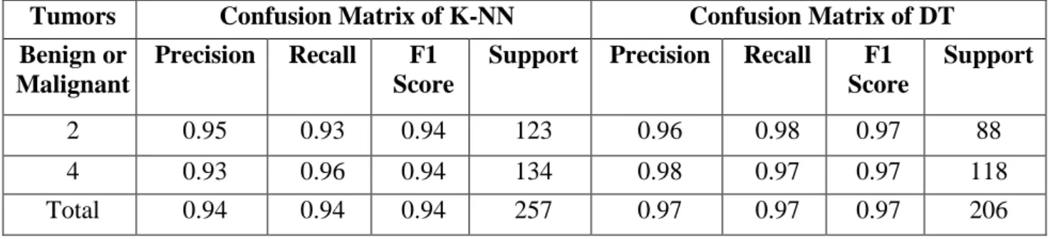
The major steps are; segmenting, removing the blobs connected to border, keep only the two largest connected components in each slice (figure 1), erosion operation with a disk of radius followed by closing operation with a disk of radius to keep the lung wall attached nodules inside the lung mask, It takes a slice as the input and returns a slice of the same size as the output which is the segmentation map of nodules. To reduce the computational power we down sized the number of input vectors in each layer to half size of the original architecture by taking edge input after finding (Table 1&2) the precision, recall, f1 score and support each corresponding slice will reduce the computation and give the percentage for detecting the lung nodules and tumors.
Table 1. Confusion matrices for both k-NN and DTrepresenting Precision, Recall, F1 score and Support.
Tumors Confusion Matrix of K-NN Confusion Matrix of DT
Benign or Malignant
Precision Recall F1
Score
Support Precision Recall F1
Score
Support
2 0.95 0.93 0.94 123 0.96 0.98 0.97 88
4 0.93 0.96 0.94 134 0.98 0.97 0.97 118
Total 0.94 0.94 0.94 257 0.97 0.97 0.97 206
Table 2. Confusion matrices for SVM representing Precision, Recall, F1 score and Support.
Tumors Confusion Matrix of SVM
Benign or Malignant
Precision Recall F1 Score Support
0 0.43 1.00 0.60 9
1 1.00 0.25 0.40 16
Total 0.79 0.52 0.47 25
Total 97.5% accuracy is achieved throughout the process. View of lung scan threshold with corresponding lung data available. Selecting the radius of the disk used for the closing operation is critical. For low values of the disk radius, the wall attached nodules kept as part of the lung wall and removed from the lung region. For high values of disk radius lung wall attached nodules were also kept inside the lung region [20].
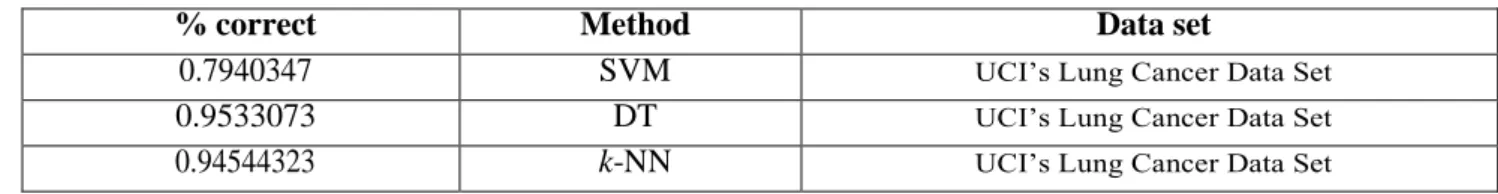
Table 3. Overall accuracy function of all three supervised inductive algorithms on test data after validation and splitting the dataset for both testing and validation to reduce the over-fitting in training to get the desired plus optimum results.
% correct Method Data set
0.7940347 SVM UCI’s Lung Cancer Data Set
0.9533073 DT UCI’s Lung Cancer Data Set
0.94544323 k-NN UCI’s Lung Cancer Data Set
But when increasing the disk radius, the part of bronchus also included as lung regions. Since nodules can also be attached to the bronchus this is desirable for some extent. But since the bronchus has similar intensities as nodules, unnecessarily inclusion of bronchus results in problems in later steps.
5. Discussion
In this paper, we describe the methods, implementation steps, and results of our project on lung cancer detection. We evaluated approach that used various machine learning techniques. In the part, we made use of a Classifier for the segmentation of potentially cancerous nodules from patient scans. A simple heuristic is used to remove false positives by keeping nodule detections only if they are detected in the slice using data mining [21]. We explored three different ways to encode the patches in this approach, and found, rather unexpectedly, that using the raw pixels yielded better results than more sophisticated methods such as autoencoders and local binary patterns. To resolve the issue of the unavailable nodule-level labels, we computed a patient-level average feature vector from the encoded patches. Using this approach, we obtained our best score and a rank of 535/1679. In the approach, we tried to reduce the number of false positives by using a classifier to combine all nodule detections for a patient [17] and segmenting it to keep the regions that have the most detections. Despite the additional step to remove false positives, the score obtained did not improve from the approach [19]. This could be explained by the fact that the nodule detection has a lot of false negatives; it is not segmenting nodule regions that should be identified and cropped. Additionally, it was seen that there are still many false positives using the classifier. This could be better addressed with a better ne-tuning of parameters like the threshold value to keep the nodules across all the slices, and the dice coefficient threshold which show how much a nodule must overlap in the lung regions to be kept as a nodule for classification. In the third approach, we used all slices for a single patient with a data mining and machine learning to exploit the volumetric data. While this approach required the least preprocessing and the least assumptions or approximations as far as extracting and labeling individual nodules are concerned, the model required excessive amounts of memory that we did not have. To handle this, we had to simplify our model significantly, which is probably what lead to the weak performance. Finally, in approach, we used a modification of approach 2 that replaced the classifier with the method described in the approach to reduce the number of false positives [21]. This lead to a slight decrease in performance compared to the second approach.
The main challenge we faced in this project was the compute and memory resources needed to handle the large size of the datasets involved. In addition, the labels provided with the main dataset were rather challenging, as they did not refer to nodule locations at all. Within the approaches described above, we explored three different methods to handle the labels: averaging nodule encodings per patient, labeling nodules with the same label given to the patient, or, finally, to not do nodule detection at all and opt instead for a model on the raw images [22-24]. Of these, the method seemed to have given the best score.
CONCLUSION
We have presented a work for lung cancer classification from UCI’s dataset for data mining volumes using combined method of classical featured based classifiers and supervised learning algorithms and approaches which includes support vector machine, k-nearest neighbor and decision trees. (table. 3) We have seen that to predict the malignancy of the overall scan we take the binary OR operation of each of these results [27-29] . That is if single nodule is turned out to be cancerous, we conclude that the overall scan as malignant. Even though the results from nodule segmentation stage is very accurate enough to predicting the locations of the nodulous regions, sometimes it is unable to predict nodule contours more precisely since we are applying some morphological operations yielding eroded contours into nodules. Therefore, the first step of this approach is the generation of nodule contours in order to accurately calculate above features.
When using this trained network for the prediction purpose of our pipeline, first we labeled the obtained data through dataset provided in nodule extraction stage. Then the center coordinates of all connected components were obtained, and sized accuracy cubes were cut around these centers. Then each of these cubes were sent through this network and the probabilities of being each of these cubes as nodules were taken to create a stack of a probability output detection of lung cancer. It can be seen that all three algorithms SVM, DT and k-NN tends to output nodules as well as large number of false positives indicating blood vessels as nodules. At the same time feature based method outputs parts of bronchus as the nodule candidates frequently. Thus, the binary mask indicating the possible nodule locations obtained through the union of them gives a lot of false positives besides the true positive nodule regions. Therefore, essential step in our classification pipeline is the false positive reduction of cancer and effective detection of lung cancer.
References
[1] RushilAnirudh, Jayaraman J Thiagarajan, Timo Bremer, and Hyojin Kim. Lung nodule detection using 3d classifier neural networks trained on weakly labeled data. In SPIE Medical Imaging, pages 978532-978532. International Society for Optics and Photonics, 2016.
[2] Dan Ciresan, Alessandro Giusti, Luca M Gambardella, and J•urgenSchmidhuber. Deep neural networks segment neuronal membranes in electron microscopy images. In Advances in neural information processing systems, pages 2843-2851, 2012.
[3] Andre Esteva, Brett Kuprel, Roberto A Novoa, Justin Ko, Susan M Swetter, Helen M Blau, and Sebastian Thrun. Dermatologist-level classification of skin cancer with deep neural networks. Nature, 542(7639):115-118, 2017.
[4] Jacques Ferlay, Isabelle Soerjomataram, Rajesh Dikshit, Sultan Eser, Colin Math-ers, MariseRebelo, Donald Maxwell Parkin, David Forman, and Freddie Bray. Cancer incidence and mortality worldwide: sources, methods and major patterns in globocan 2012. International journal of cancer, 136(5):E359-E386, 2015.
[5] Rotem Golan, Christian Jacob, and J•orgDenzinger. Lung nodule detection in images using deep classifier neural networks. In Neural Networks (IJCNN), 2016 International Joint Conference on, pages 243-250. IEEE, 2016.
[6] Metin N Gurcan, BerkmanSahiner, Nicholas Petrick, Heang-Ping Chan, Ella A Kazerooni, Philip N Cascade, and LubomirHadjiiski. Lung nodule detection on thoracic computed tomography images: Preliminary evaluation of a computer-aided diagnosis system. Medical Physics, 29(11):2552{2558, 2012}.
[7] Devinder Kumar, Alexander Wong, and David A Clausi. Lung nodule classification using deep features in images. In Computer and Robot Vision (CRV), 2015 12th Conference on, pages 133-138. IEEE, 2015.
[8] Fan Liao and Chunxia Zhao. Improved fuzzy c-means clustering algorithm for automatic detection of lung nodules. In Image and Signal Processing (CISP), 2015 8th International Congress on, pages 464-469. IEEE, 2015.
[9] NegarMirderikvand, MarjanNaderan, and Amir Jamshidnezhad. Accurate automatic localisation of lung nodules using graph cut and snakes algorithms. In Computer and Knowledge Engineering (ICCKE), 2016 6th International Conference on, pages 194-199. IEEE, 2016.
[10] Olaf Ronneberger, Philipp Fischer, and Thomas Brox. Classifier: convolutional networks for biomedical image segmentation. In International Conference on Medical Image Computing and Computer-Assisted Intervention, pages 234-241. Springer, 2015.
[11] Arnaud ArindraAdiyosoSetio, Alberto Traverso, Thomas de Bel, Moira SN Berens, Cas van den Bogaard, PiergiorgioCerello, Hao Chen, Qi Dou, Maria EvelinaFantacci, Bram Geurts, et al. Validation, comparison, and combination of algorithms for automatic detection of pulmonary nodules in computed tomography images: the luna16 challenge. arXiv preprint arXiv:1612.08012, 2016.
[12] Sumit K Shah, Michael F McNitt-Gray, Sarah R Rogers, Jonathan G Goldin, Robert D Suh, James W Sayre, Iva Petkovska, Hyun J Kim, and Denise R Aberle. Computer-aided diagnosis of the solitary pulmonary nodule 1. Academic radiology, 12(5):570-575, 2015.
[13] Wei Shen, Mu Zhou, Feng Yang, Caiyun Yang, and JieTian. Multi-scale convolutional neural networks for lung nodule classification. In International Conference on Information Processing in Medical Imaging, pages 588-599. Springer, 2016.
[14] Akira Motohiro, Hitoshi Ueda, Hikotaro Komatsu, NoboruYanai, and Takashi Mori, “Prognosis of non-surgically treatedclinical stage I lung cancer patients in Japan,” Lung CancerJournal, vol.36, issue.1, pp.65-69, April 2016.
[15] MariosAnthopoulos, StergiosChristodoulidis, Lukas Ebner,Andreas Christe and StavroulaMougiakakou, “Lung PatternClassification for Interstitial Lung Diseases Using a DeepConvolutional Neural Network,” IEEE
Transaction on MedicalImaging, vol.35, May 2016.
[16] J. AlameluMangai, JagadishNayak and V. Santhosh Kumar;“A Novel Approach for Classifying Medical Images Using DataMining Techniques,” International Journal of Computer Scienceand Electronics
Engineering, vol.1, issue.2 2013.
[17] PetrBerka, Jan Rauch and DjamelAbdelkaderZighed,“Ontologies in the Health Field,” in Data Mining
and MedicalKnowledge management: Cases and Application, Hershey, UnitedStates: IGI Global, March 2011,
pp. 37-56.
[18] PetrBerka, Jan Rauch and DjamelAbdelkaderZighed, “Cost-Sensitive Learning in Medicine,” in Data
Mining and MedicalKnowledge management: Cases and Application, Hershey, UnitedStates: IGI Global,
March 2017, pp. 57–75.
[19] PetrBerka, Jan Rauch and DjamelAbdelkaderZighed,“Classification and Prediction with Neural Networks,” in DataMining and Medical Knowledge management: Cases andApplication, Hershey, United States: IGI Global, March 2017, pp.76–107.
[20] Thomas Erl, WajidKhattak, Paul Buhler, “Understanding BigData,” in Big Data Fundamentals, Crawfordsville, Indiana; USA:RR Donnelley, December 2015, pp. 21–35.
[21] Cortes Corinna and Vapnik Vladimir, "Support-vectornetworks," Machine Learning, vol.20, issue.3, pp.273–297, September 2016.
[22]Tsung-Yu Lin, AruniRoyChowdhury, SubhransuMaji,“Bilinear CNN Models for Fine-Grained Visual Recognition,” inIEEE International Conference on Computer Vision(ICCV),2015, pp. 1449-1457.
[23] Abdulshaheed, H.R., Binti, S.A., and Sadiq, I.I., 2018. A Review on Smart Solutions Based-On Cloud Computing and Wireless Sensing. International Journal of Pure and Applied Mathematics, 119 (18), pp.461– 486.
[24] Shibghatullah, A.S. and Barazanchi, I. Al, 2014. An Analysis of the Requirements for Efficient Protocols in WBAN. Journal of Telecommunication, Electronic and Computer Engineering, 6 (2), pp.19–22.