Implementing Spatial Data Analysis
Software Tools in
R
Roger Bivand
Economic Geography Section, Department of Economics, Norwegian School of Economics and Business Administration, Bergen, Norway
This article reports on work in progress on the implementation of functions for spatial statistical analysis, in particular of lattice/area data in theRlanguage environment. The underlying spatial weights matrix classes, as well as methods for deriving them from data from commonly used geographical information systems are presented, handled using other contributedRpackages. Since the initial release of some functions in 2001, and the release of thespdeppackage in 2002, experience has been gained in the use of various functions. The topics covered are the ingestion of positional data, exploratory data analysis of positional, attribute, and neighborhood data, and hypothesis testing of autocorrelation for univariate data. It also provides information about community building in usingRfor analyzing spatial data.
Introduction
Changes in scientific computing applied to data analysis are less rapid than in many consumer fields. Underlying technologies are well known, and have been available for decades. The visible changes are much more in the burgeoning of online and virtual scientific communities and in the availability of cross-platform applications, giving many more researchers, scientists, and students access to implementations of methods that, until recently, only appeared in journal articles. In this context, Anselin, Florax, and Rey (2004), Pebesma (2004), and Grunsky (2002) have recently drawn attention to the R data analysis and statistical programming environment as an emerging area of promise for the social and environmental sciences, and Waller and Gotway (2004) provide a selectedRcode to support their book on applied spatial statistics for public health data.
This article was first prepared for the CSISS specialist meeting on spatial data analysis software tools, Santa Barbara, CA, May 10–11, 2002.
Correspondence: Roger Bivand, Economic Geography Section, Department of Economics, Norwegian School of Economics and Business Administration, Helleveien 30, N-5045 Bergen, Norway
e-mail: [email protected]
Ris an implementation of theSlanguage;Rwas initially written by Ross Ihaka and Robert Gentleman (Ihaka and Gentleman 1996; R Development Core Team 2005).S-PLUS is a proprietary implementation ofS; as bothRandS-PLUSare implementations of the same underlying language, they are often able to execute the same interpreted code. R follows most of the Blue and White books that describeS(Becker, Chambers, and Wilks 1988; Chambers and Hastie 1992), and also implements parts of the more recent Green Book (Chambers 1998). R is available as free software under the terms of the Free Software Foundation’s GNU General Public License in source code form. It compiles and runs out of the box on a wide variety of Unix platforms and similar systems (including GNU/Linux). It also compiles and runs on Windows systems and MacOSX, and as such provides a functional cross-platform distribution standard for software and data. A good introduction is provided by Dalgaard (2002).
It is fair to say that the statistical and data-analytic interests of theRcommunity are catholic and rigorous, and participants are enthusiastic, challenging the perceived barriers between proprietary and open-source software in the interests of better, more timely, and more professional analysis in the proper sense of the word. Naturally, other and overlapping communities share these qualities; Matlab users interact and share code willingly, Python programmers do the same, as do users and developers working in a range of other language environments like Stata. In all of these cases, users and developers share interests in data analysis, in which participants in different fields can draw on each other’s experience.
The following discussion has two equal threads. The first is to learn from theR
project about how an analytic and infrastructure-providing open-source commu-nity has achieved critical mass to enable mutually beneficial sharing of knowledge and tools. The second is to apply relevant lessons to the development of software tools for spatial data analysis in the context of theRproject, and to give examples from the progress made so far for areal data.
At the time of writing (October 2004), a search of the R site for ‘‘spatial’’ yielded 1219 hits, almost three times the 447 hits found in May 2002. As Ripley (2001) comments, some of the hesitancy that was observable in contributing spatial analysis packages to R was due to the availability of the S-PLUS SpatialStats module: duplicating existing work (including geographic information system [GIS] integration) had not seemed fruitful. Over the recent period, however, a number of packages have been released on CRAN, the Comprehensive RArchive Network (http://cran.r-project.org), in all three areas of spatial data analysis (point patterns, continuous surfaces, and lattice data) as well as in accessing geographical data in common GIS formats.
An early package in point pattern and continuous surface analysis,spatial, was contributed toRfrom the first edition of Venables and Ripley (2002)—now in its fourth edition. Initially written forSandS-PLUS, it was ported toRby Brian Ripley following work by Albrecht Gebhardt. Descriptions of some of the packages available are given in notes inR News(Bivand 2001; Ripley 2001), while a more
dated survey was made by Bivand and Gebhardt (2000), reflecting the situation at that time.Ras a whole is experiencing rapid growth in the number of contributed packages, and because it can be difficult to obtain an overview of relevant software, authors of spatial statistics software agreed to set up a Web site. This has been in operation since mid-2003, has an associated mailing list, and currently can be reached by searching Google with the string, ‘‘R spatial,’’ or from an entry on the navigation bar on the left of the mainRWeb site (http://www.r-project.org/Rgeo). Rather than duplicate this information, summarized in Table 1, the next section will be concerned with highlighting features of theRimplementation of Sthat are of potential value for implementing data analysis functions.
Ras an environment for implementing data analysis functions
In the terminology used in theRproject, the programming environment is provided as a program interpreting the language, managing memory, providing services, and running the user interface (command line, history mechanisms, and graphics windows). It is worth noting that the language supports the use of expressions as function arguments, allowing considerable fluency in command-line interaction and function writing. There is a clearly defined interface to this program, permitting additional compiled functions to be dynamically loaded, and interpreted functions to be introduced into the list of known objects. By default on program startup, the
basepackage is loaded, followed by autoloaded packages, and other packages are loaded at will. R distributions are accompanied by a set of packages, available by default and providing foundation functions and services, and a larger recom-mended collection.
Contributed packages provide a powerful vehicle for distributing additional code, and their structure encourages the extension of the catalogue of functions
Table 1 Packages for Spatial Data Analysis Linked from the Web Site. Packages are on CRAN, Other Packages are on Sourceforge
Functionality Packages
Read shapefiles maptools, shapefiles
Read other vector formats RArcInfo, Rmap
Read raster formats rgdal
GIS integration GRASS
Draw maps maptools, RArcInfo,Rmap,maps,sp
Project maps mapproj, Rmap,spproj
Spatial data classes sp
Point patterns spatial, spatstat, splancs
Geostatistics spatial, gstat, sgeostat, geoR, geoRglm, fields
Areal/lattice spdep, DCluster,spgwr
available to users. Venables and Ripley (2000) cover S programming in detail, including a description of packaging mechanisms inR; other information is to be found in online documentation, also included in the software distribution. AsRis an open source, the ultimate documentation is the source code itself, albeit for those willing and able to read it. This is a statement of position with an academic attitude, presupposing that at least academics ought not to use tools they are not prepared to try to understand if that understanding is crucial to their work. In this setting, understanding how algorithms are implemented in code is seen as a part of applied science, and the link between data analysis, good research practice, and programming is acknowledged.
Packages are contributed in source form, and may also be distributed in compiled, binary form. Most, although not all, source packages on CRAN are built as binaries in an automated process for Windows and MacOSX platforms; on Unix (now also including MacOSX), and GNU/Linux platforms, users are more likely to have access to appropriate build trains. Issuing the update.packages() command on Windows and MacOSX platforms in anRsession online permits the updating of binary installed packages from CRAN (either the master site or a closer mirror);install.packages()with a character vector of package names as an argument installs the required binary packages from CRAN. On Unix and GNU/ Linux platforms, the same functions update and install source packages, building them locally.
These mechanisms provide users with one of the key benefits of open-source development: access to software subject to rapid release cycles. Often, package maintainers are able to correct bugs in code or documentation, or incorporate user-contributed functionality, within days; this has advantages and disadvantages. During a teaching course, or a research project, theRrelease is likely to change (four to five minor version changes per year), and package versions may also change, sometimes rapidly as work progresses or because of community contribu-tions or pressure, often whenRversions change. Recording the versions used for results that may need to be verified is always sensible; if needed for the reconstruc-tion of results, older versions of Rand all CRAN packages may be downloaded from CRAN.
A minimal source package contains a directory of files of interpreted functions, and a directory of files of documentation of this code. All functions should be fully documented, and must be if the package is to be distributed through CRAN. It is customary for the documentation to include example sections that can be executed to demonstrate what the function does; typically, data sets distributed with the base package are used, if possible. It is a requirement for distribution on CRAN that the examples run without error—not a guarantee that the implementations are correct with respect to the initial formal description of the method, but at least that running them does not terminate with an error. If one chooses to use domain-specific data sets, then the package will contain a further directory with the necessary data files, which in turn are documented in the help file directory. The interpretedRcode can
of course be read within the context of the user interface, and functions may be edited, saved to user files, and sourced back into the program.
In some circumstances, it is desirable to move the internal computations of a function to a compiled language, although, as we will see, this is not an absolute requirement because the built-in internal functions themselves interface highly optimized and heavily debugged compiled code. In this case, a source directory will also be present, with C, C11, or Fortran 77 source files. Here, it is sufficient to mention the possibility of a dynamically loading user-compiled shared object code, and the usefulness ofRheader files in C, in particular providing direct access toR
functions.Rdata objects may be readily passed to and from user functions, andR
memory allocation mechanisms may be called from such user-compiled functions. If required, theRcode can even be executed in such user-compiled functions.
For instance,Rprovides afactorobject definition for categorical variables, with a character vector of level labels and an integer vector of observation values pointing to the vector of levels. In the GRASS/R compiled interface using GRASS library functions (Bivand 2000), moving categorical raster data between R and GRASS is accomplished fast and fully preserving labels by operating on Rfactor objects in C functions. WithinR, functions are written to use object classes, for example, the factor class, to test for object suitability, or in many modeling situations to convert factors into appropriate dummy variables. The use of classes inRfor spatial data analysis is discussed in more depth by Bivand (2002).
Another example is the widespread use of the formula object abstraction. Formulae are written in the same way for models of many kinds. The left- and right-hand sides are separated by the tilde (), and the right-hand side may express interactions and conditioning. If a factor is included on the right-hand side, the model matrix will contain the necessary dummy variables. Formulae are used from multiple box plots, through cross-tabulations, lattice (Trellis) graphics using con-ditioning to explore higher-dimensional relationships, to all forms of model-fitting functions. The formula abstraction was introduced to theSlanguage in Chambers and Hastie (1992), and is used in the spatial statistics packages as well; see Pebesma (2004) for examples.
Users and developers can create new classes for which the class method dispatch mechanism can be invoked. The summary() function appears to be a single function, but in fact calls appropriate summary functions based on the class of the first argument; the same applies to theplot()andprint()functions. The extent to which spatial data analysis packages use class- and method-based functions varies, mostly depending on the age of the code and on the potential value of such revisions; status as of early 2003 is reviewed in Bivand (2003). At present, some do not use classes—assuming specific list structures for spatial data, others use old-style classes specific to the package (also known as S3 classes, described in Chambers and Hastie 1992, appendix A, pp. 455–80), and a few have begun to use new-style classes (S4classes, described in Chambers 1998, chapters 7–8; Venables and Ripley 2002, chapter 5). New-style classes mandate the
structure of a class by design, so that content creep is not permitted, and functions using the classes can be written cleanly, because the structure of the object is known from its published definition.
Pebesma (2004) presents work in progress on designingS4classes for spatial data, which is hosted on SourceForge and can be accessed from the R spatial projects Web site; publication of the foundation classes as packagespon CRAN has now occurred. These classes will provide a set of containers for data import and export on the one hand, and a standardized set of objects for analysis functions on the other. It is not clear how much GIS functionality should be available withinR
natively, so the availability of data objects that can be moved readily to external GIS for processing and modification is necessary. On the other hand, GIS (perhaps with the exception of GRASS) do not let the analyst get as close to the data as is possible inR.
As has already been indicated indirectly, much of the added value of the R
project extends beyond the standard functionality of the language and program-ming environment. The archive network is such an extension, as are the package-checking mechanisms (in the tools package). Together with the test suites, they have been developed to facilitate quality control of the core system rather than user-contributed packages, but because the same standards are used, the con-tributed packages also benefit in terms of organization and coherence. Another useful spillover from package contributors to the core team is that all contributed packages on CRAN are verified nightly against the code bases of the released version of R, the patched version, and the development version—which will become the next full release. This means that the core team can track the effects of changes in the compute engine on a large body of code that has run without evident error at some previous point in time. Of course, only use shows how close the implementations are to the underlying formal and/or numerical methods, as with other software, so these checks do not try to validate the procedures involved. The underlying numerical functions and random number generators are, however, well proven.
Thetoolspackage also contains functions to support literate statistical analysis, written to contain both documentation and the specification of procedures actually run to generate results (text, tabular, and graphical). TheSweave()function runs on a file containing, in the LaTeX andRcase, a marked-up mixture of LaTeX and
Rcode, producing a file in LaTeX including verbatim code chunks, the output of the commands issued, and files with tables or graphics in suitable formats for inclusion. Leisch and Rossini (2003) argue that, with increasing dependence on the settings needed to replicate results, for instance, the specific random number generator and seed used, such literate analysis techniques are needed for repro-ducible research. This infrastructure has been extended and implemented as a less terse way of documenting packages contributed to R, in documents known as vignettes, and used extensively in the Bioconductor project (Gentleman et al. 2005). Vignettes also contain code that is verified on the same basis as help page
examples. This article has been written using the literate statistical analysis support available inR.
On the graphics side,Rdoes not provide dynamic linked visualization, as the graphics model is based on drawing on one of a number of graphics devices. R
does provide the more important tools for graphical data analysis, although no mapping is present as yet in general terms. TheRspatial analysis Web site referred to above covers packages on CRAN for mapping using the legacy S format, shapefiles, and ArcInfo binary files, but each of these packages uses separate mechanisms and object representations at present. Panelled (Trellis) graphics are provided in thelatticepackage, and is now mature and makes available many of the tools needed for analyzing high-dimensional data in a reproducible fashion. This can be contrasted with dynamically linked visualization, which can be difficult to render as hard copy. Graphics are extensible at the user level in many ways, but are more for viewing and command-line interaction than for pointer-driven interaction.
Implementation examples
In this section, we will use some of the implementation details of spdep to exemplify the internal workings of an R package; this package is a workbench for exploring alternative implementation issues, and bug reports, contributions, and criticisms are very welcome. The illustrations will draw on canonical data sets for areal or lattice data, many of which are included in the package to provide clear comparisons with the underlying literature. Using the reproducible research format,
Rcommands are preceded by the main prompt4, or the continuation prompt1, and are expressed in italic; output is not preceded by a prompt and is set in normal style.
Most of the world as seen by data analysis software still resembles a flat table, and the most characteristic object class inRat first seems to be the data frame. But a data frame, a rectangular flat table with row and column names, and made up of columns of types including numeric, integer, factor, character, and logical, and with other attributes, is in fact a list. Lists are very flexible containers for data of all kinds, including the output of functions. They form the workhorse for many spatial data objects, such as, for example, polygons read intoRfrom shapefiles using the
maptoolspackage.
We will be using the North Carolina Sudden Infant Death Syndrome (SIDS) data set, which was presented first in Symons, Grimson, and Yuan (1983), analyzed with reference to the spatial nature of the data in Cressie and Read (1985), expanded in Cressie and Read (1989) and Cressie and Chan (1989), and used in detail in Cressie (1993). It is for the 100 counties of North Carolina, and includes counts of numbers of live births (also non-White live births) and numbers of sudden infant deaths, for the 1974–1978 and 1979–1984 periods. In Cressie and Read (1985), a listing of county neighbors based on shared boundaries (contiguity) is
given, and in Cressie and Chan (1989), and in Cressie (1993, pp. 386–89), a different listing is given based on the criterion of distance between county seats, with a cutoff at 30 miles. The county seat location coordinates are given in miles in a local (unknown) coordinate reference system. The data are also used to exemplify a range of functions in theS-PLUSspatial statistics module user’s manual (Kaluzny et al. 1996).
Presenting the data
The data from the sources referred to above are collected in thenc.sidsdata set inspdep. But to map it, we also need access to data for the county boundaries for North Carolina; this has been made available in themaptoolspackage (originally written by Nicholas Levin-Koh) in shapefile format (these data are taken with permission from: http://sal.uiuc.edu/datasets/sids.zip). The package versions used here were:spdep0.2–22 andmaptools0.4–7,Rversion: 2.0.0. The position data are known to be geographical coordinates (longitude–latitude in decimal degrees) and are assumed to use the NAD27 datum.
The shapefile format presupposes that there are at least three files with extensions
.shp, .shx, and .dbf, where the first contains the geometry data, the second contains the spatial index, and the third contains the attribute data. They are required to have the same name apart from the extension, and are read usingread.shape(). By default, this function reads in the data in all three files, although it is only given the name of the file with the geometry.4library(spdep)
Loading required package: tripack
Loading required package: maptools
4nc. sids.shpo- read.shape(system.file(‘‘shapes/sids.shp’’, package5‘‘maptools’’),
1 verbose5FALSE)
4ncpolyso- Map2poly(nc.sids.shp, raw5FALSE)
The imported object in Rhas classMap, and is a list with two components, Shapes, which is a list of shapes, and att.data, which is a data frame with tabular data, one row for each shape inShapes. We convert the geometry format of theMapobject to that of apolylistobject, which will be easier to handle. The object is also put through sanity checks if therawargument is set toFALSE; many shapefiles in the wild do not conform to the specification that hole boundary coordinates be listed anti-clockwise, information that is needed for plotting.
The polylist is an S3 class with additional attributes, and is a list of polygons (possibly multiple polygons), each with further attributes. An S4 class definition built on polylist is included in sp, and is used in the forthcoming
spgwrpackage for geographically weighted regression. Using theplot()function for polylist objects frommaptools, we can display the polygon boundaries, shown as the background in Fig. 1.
While point pattern data can exist happily within flat tables, as indeed can point locations with attributes as used in the analysis of continuous surfaces, as well as time series, the specific structuring data object of lattice data analysis describing the neighborhood relations between observations cannot. When the weights matrix is represented as a matrix, it is very sparse, and the analysis of moderate-to-larger data sets may be impeded. This provides one reason for supplementing the existing S-PLUSspatial statistics module for lattice data. In theS-PLUScase, weights are represented sparsely in a data frame, with four columns: weights matrix element row index, column index, value, and (optionally) the order of the weights matrix when multiple matrices are stored in the same data frame. While this provides a direct route to sparse matrix functions for finding the Jacobian, and for matrix multiplication, it makes the retrieval of neighborhood relations awkward for other needs. Here, it was found to be simpler to create a hierarchy of class objects leading to the same target, but also open to many operations at earlier stages.
The basic building block is, as with thepolylistclass, the list, with each list element being an integer vector containing the indices of its neighbors in the present definition. The list is of classnb, and has a character region ID attribute, to provide a mapping between the region names and indices. These lists may be read in as legacy GAL-format files, enhanced GAL and GWT format files as written by GeoDa, and Matlab sparse matrices saved as text files, or produced by collapsing input weights matrices to lists. They may be generated from lists of polygon perimeter coordinates or from matrices of point coordinates representing the regions under analysis. Nicholas Levin-Koh contributed a number of useful graph-derived functions, so that there is now quite a choice with regard to creating lists of neighbors; further details may be found in Bivand and Portnov (2004). Class
nbhasprint(),summary(), andplot()functions.
–84 –82 –80 –78 –76 33 34 35 36 37
Cressie and Chan 1989 dnearneigh different links
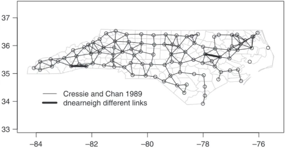
Figure 1. Overplotting shapefile boundaries with 30 mile neighbor relations as a graph; two extra links are shown from replicating the neighbor scheme with the original input data.
We will now access the data set reproduced from Cressie and collaborators, included in spdep, and add the neighbor relationships used in Cressie and Chan (1989), stored asnbobjectncCC89.nb, to the background map as a graph, shown in Fig. 1. The criterion used for two counties to be considered neighbors was that their county seats should be within 30 miles of each other, which is not fulfilled for two Atlantic coast counties. Columnsc("lon," "lat")in data framenc.sids contain the geographical coordinates of the county seats (vector and matrix indices are given in single square brackets, and list element indices in double square brackets). Note that theplot() function is being used for class-based methods dispatch, with one function being used to display objects of thepolylist class like ncpolys and a different function to display the neighbors list ncCC89.nb object of class nb. One of the reasons why it is sometimes difficult to replicate classic results is that it can be difficult to regenerate neighbor relations even given area boundaries or point coordinates. This is illustrated here by running
dnear-neigh() on the local projected coordinates of the county seats in columns
c("east," "north")(Cressie 1993, pp. 386–89); two links are added to the published list of neighbors, illustrated by plotting the neighbor list resulting from computing the difference between the two lists.
4data (nc.sids)
4new30o- dnearneigh(as.matrix(nc.sids[, c(‘‘east’’,‘‘north’’)]),
1 d1 50, d2530, row.names 5nc.sids$CNTY.ID) 4plot(ncpolys, border5 ‘‘grey’’)
4plot(ncCC89.nb, as.matrix(nc.sids[, c(‘‘lon’’,‘‘lat’’)]), add 5TRUE) 4plot(diffnb(ncCC89.nb, new30, verbose 5FALSE), as.matrix(nc.sids[,
1 c(‘‘lon’’,‘‘lat’’)]), points5FALSE, add5TRUE, lwd53)
A print of the neighbor object shows that it is a neighbor list object, with a very sparse structure—if displayed as a matrix, only 3.94% of cells would be filled (simply typing an object name at the interactive command prompt prints it). We should also note that this neighbor criterion generates two counties with no neighbors, Dare and Hyde, whose county seats were more than 30 miles from their nearest neighbors. The card() function returns the cardinality of the neighbor sets.
4ncCC89.nb
Neighbour list object:
Number of regions: 100 Number of nonzero links: 394 Percentage nonzero weights: 3.94
Average number of links: 3.94 2 regions with no links:
2000 2099
4as.character(nc.sids.shp$att.data$NAME)[card(ncCC89.nb)550] [1]‘‘Dare’’ ‘‘Hyde’’
Probability mapping
Rather than reviewing functions for measuring and modeling spatial dependence in thespdeppackage, we will focus on support for the analysis of rates data, starting with problems in probability mapping. Typically, we have counts of the incidence by spatial unit, associated with counts of populations at risk. The task is then to try to establish whether any spatial units seem to be characterized by higher or lower counts of cases than might have been expected in general terms (Bailey and Gatrell 1995; Waller and Gotway 2004).
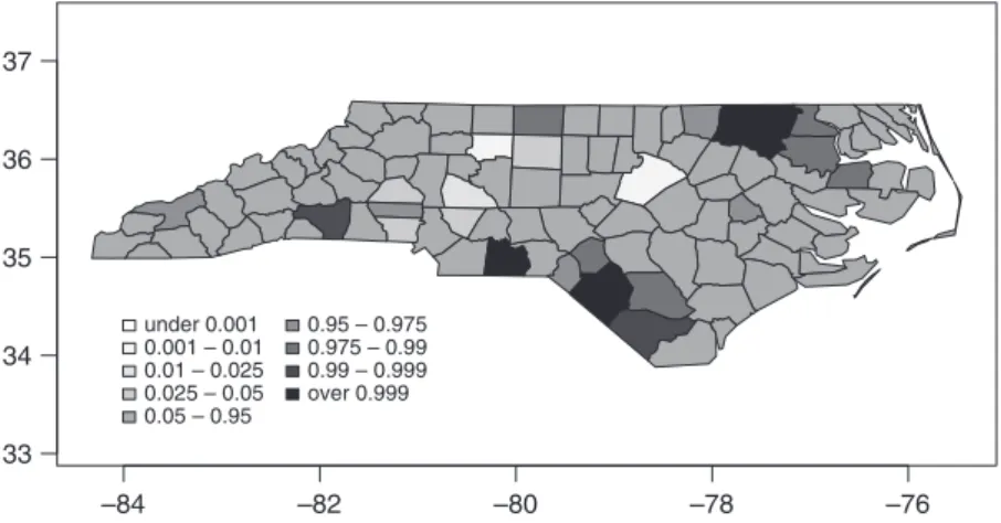
An early approach by Choynowski (1959), described by Cressie and Read (1985) and Bailey and Gatrell (1995), assumes, given that the true rate for the spatial units is small, that as the population at risk increases to infinity, the spatial unit case counts are Poisson, with the mean value equal to the population at risk times the rate for the study area as a whole. The probmap() function returns raw (crude) rates, expected counts (assuming a constant rate across the study area), relative risks, and Poisson probability map values calculated using the standard cumulative distribution function ppois(). Counties with observed counts lower than expected, based on population size, have values in the lower tail, and those with observed counts higher than expected have values in the upper tail, as Fig. 2 shows. Here, we will use the gray sequential palette, available inRin theRColorBrewerpackage (http://colorbrewer.org), and the basefindInterval()function to assign colors to probability map values.
–84 –82 –80 –78 –76 33 34 35 36 37 under 0.001 0.001 – 0.01 0.01 – 0.025 0.025 – 0.05 0.05 – 0.95 0.95 – 0.975 0.975 – 0.99 0.99 – 0.999 over 0.999
Figure 2. Probability map of North Carolina counties, SIDS cases 1974–78, reproducing Kaluzny et al. (1996, p. 67, Figure 3.28).
4library(RColorBrewer)
4pmapo– probmap(nc.sids$SID74, nc.sids$BIR74)
4brkso– c(0, 0.001, 0.01, 0.025, 0.05, 0.95, 0.975, 0.99, 0.999,
1 1)
4colso– brewer.pal(length(brks) – 1,‘‘Greys’’)
4plot(ncpolys, col5cols[findInterval(pmap$pmap, brks, all.inside5TRUE)],
1 forcefill5FALSE)
Marilia Carvalho (personal communication) and Virgilio Go´mez Rubio and co-authors (Go´mez-Rubio, Ferra´ndiz, and Lo´pez 2005) have pointed out the unusual shape of the distribution of the Poisson probability values (Fig. 3), echoing the doubts about probability mapping voiced by Cressie (1993, p. 392): ‘‘an extreme value . . . may be more due to its lack of fit to the Poisson model than to its deviation from the constant rate assumption’’; see also Waller and Gotway (2004, p. 96): ‘‘. . . it may not be possible to distinguish deviations from the constant risk assumption from lack of fit of the Poisson distribution.’’ There are many more high values than one would have expected, suggesting perhaps overdispersion, that is, that the ratio of the mean and variance is larger than unity.
One ad hoc way to assess the impact of the possible failure of our assumption that the counts follow the Poisson distribution is to estimate the dispersion by fitting a general linear model using the quasi-Poisson family and log link to the observed counts including only the intercept (null model) and offset by the expected counts (suggested by Marilia Carvalho and associates). The dispersion is equal to 2.2784, much greater than unity; this can be checked because R provides access to a wide range of model-fitting functions. Likelihood ratio and Dean tests also used by Go´mez-Rubio, Ferra´ndiz, and Lo´pez (2005) confirm the presence of
0.0 0.2 0.4 0.6 0.8 1.0 0 5 10 15 20
serious overdispersion—these tests will be included in a forthcoming release of
DCluster.
Empirical Bayes smoothing
So far, none of the maps presented has made use of the spatial dependence possibly present in the data. A further step that can be adopted is to map Empirical Bayes estimates of the rates, which are smoothed in relation to the raw rates (see Waller and Gotway 2004, pp. 90–104, for a full discussion). The underlying question here is linked to the larger variance associated with rate estimates for counties with small populations at risk compared with counties with large populations at risk. Empirical Bayes estimates place more credence on the raw rates of counties with large populations at risk, and modify them much less than they modify rates for small counties. In the case of small populations at risk, more confidence is placed in either the global rate for the study area as a whole, or for local Empirical Bayes estimates, in rates for a larger moving window including the neighbors of the county being estimated. Thespdeppackage provides an Empirical Bayes smoother as function EBest() using the method of moments (Marshall 1991), DCluster
providesempbaysmooth()using iterations (Clayton and Kaldor 1987), andspdep
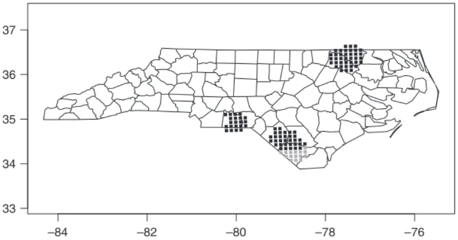
provides a local Empirical Bayes smoother initially contributed by Marilia Carval-ho,EBlocal(), following Bailey and Gatrell (1995, p. 307, pp. 328–30); this is an implementation similar to that in GeoDa (Anselin, Syabri, and Kho 2006). Fig. 4 shows the result of runningEBlocal()on the North Carolina 1974–78 SIDS data set. Like other relevant functions inspdep,EBlocal() adopts azero.policy argument to allow missing values generated for spatial units with no neighbors to be passed through (see also Bivand and Portnov 2004).
–84 –82 –80 –78 –76 33 34 35 36 37 under 2 2 – 2.5 2.5 – 3 3 – 3.5 over 3.5
Figure 4. Local Empirical Bayes estimates for SIDS rates per 1000 using the 30-mile county seat neighbors list; no local estimate is available for the two counties with no neighbors, marked by stars.
Scanning local rates
The DCluster package by Virgilio Go´mez-Rubio is one of several packages contributed toR that use the objects introduced in spdep and maptools; others areade4andadehabitatfor the analysis of environmental data.DClusterprovides a range of cluster scan tests, including many of those presented in Waller and Gotway (2004, pp. 174–83, 205–22). The example used here is Openshaw’s Geographical Analysis Machine based on Openshaw et al. (1987), and with a choice of cluster-testing functions and arguments as documented in the package.
4library(DCluster)
Loading required package: boot
4DC.sidso– data.frame(Observed5nc.sids$SID74, Expected5 pmap$expCount,
1 x 5 nc.sids$x, y 5 nc.sids$y)
4sidsgamo– opgam(data 5 DC.sids, radius5 30, step 5 10, alpha5 0.002) As its first argument, theopgam() function adopts a data frame of observed and expected counts, and requires projected coordinates of points representing the polygons within which data were collected, here Universal Transverse Mercator (UTM) zone 18 coordinated of the country seats. Fig. 5 shows the results of running the function using the North Carolina SIDS data on a 10 km grid and a cut-off radius of 30 km, for test results ofao0.002. The similarities between Figs. 4 and 5 suggest that in 1974–78, more SIDS cases were being observed in the highlighted counties than should have been expected for their populations at risk.
–84 –82 –80 –78 –76 33 34 35 36 37
Figure 5. Geographical Analysis Machine results for circle radius 30 km, and grid step 10 km, run on UTM county seat coordinates, reprojected onto geographical coordinates for display, gray symbols, 0.002a0.001; black symbols,ao0.001.
Adjustments to Moran’sI
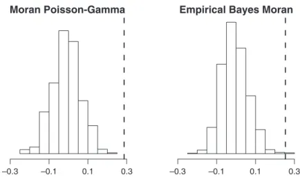
TheDClusterpackage also contains a number of interesting innovations to standard measures of spatial autocorrelation, such as Moran’sI, permitting the statistic to be tested not only under assumptions of normality or randomization, or using Monte Carlo tests—which are equivalent to a permutation bootstrap—but using para-metric bootstrapping for three models of the data: multinomial, Poisson, and Poisson-Gamma. Finally, we can calculate the adjusted Moran’sIstatistic (Assun-c¸a˜o and Reis 1999), for the counts and populations at risk, assessing its significance by simulation, implemented as functionEBImoran.mc() inspdep using Monte Carlo simulation, which is equivalent to a permutation bootstrap. For the purposes of reproducible research, the random number generator and its seed are fixed. Fig. 6 shows histograms of the outcomes of the Moran Poisson-Gamma parametric bootstrap and the Empirical Bayes Moran Monte Carlo simulation, both for 999 replications.
The test results leave no doubt that there is considerable spatial dependence in the pattern of rates across the state. This result does not, however, tell us anything about clustering, more that neighbors have similar values, perhaps reflecting the nonstationarity reported by Cressie and Read (1985). At present, methods such as those proposed by Lawson, Browne, and Vidal Rodeiro (2003), Haining (2003), and Waller and Gotway (2004) involving Markov Chain Monte Carlo (MCMC) and multilevel modeling may be preferred, although hereRmay be used for analysis and/or to pre- and postprocess data.
Opportunities for advancing spatial data analysis inR
There seem to be four main opportunities for advancing spatial data analysis inR. The first is the vitality and rapid development ofRitself, now available on all major
Moran Poisson-Gamma
–0.3 –0.1 0.1 0.3
Empirical Bayes Moran
–0.3 –0.1 0.1 0.3 Figure 6. Moran Poisson-Gamma parametric bootstrap and the Empirical Bayes Moran Monte Carlo simulation results; observed statistics are marked by dashed vertical lines.
platforms, and supporting the release and distribution of contributed software packages through the archive network. This is assisted by the open-source devel-opment model adopted by the R project, which certainly reduces the cost of acquisition, and permits local customization where needed. It is also noticeable that take-up in underfunded teaching and research settings, such as developing countries, is occurring rapidly.
The second is the reproducible research thread present in communities like those using Matlab, S-PLUS, or R: certainly, statisticians are used to having to reveal their journaled procedures. This applies in particular in biostatistics, where the consequences of the application of erroneous or inappropriate procedures can be serious. But it also extends to other areas of analysis where peer review and insight is sought and valued, including spatial data analysis, at least partly through joint work with epidemiologists.
The third opportunity is that it seems that relatively more applied statisticians are viewing spatial data analysis with more sympathy and interest, although they may be frustrated both by data formats (the spatial position is much less system-atically recorded than time) and by internal debates within quantitative geography or geostatistics. This opportunity means that if object structures needed to analyze spatial data can be provided and documented in a language environment that applied statisticians like and understand, then they can join in the development and implementation of methods of analysis.
The fourth opportunity stems from the spatial data analysis community itself, which is capable of working together and exchanging ideas. From a period in which geographical information systems, and later geocomputation and geogra-phical information science, have been the agenda setters, there seems to be interest in trying things out, in expressing ideas in code, and in encouraging others to apply the coded functions in teaching and applied research settings. Having good ideas is no longer quite enough; their quality becomes apparent when they achieve implementation in applied fields, especially outside their fields of origin.
Acknowledgements
I thank the anonymous referees for their comments. I also thank the contributors to
spdep, including, Luc Anselin, Andrew Bernat, Marilia Carvalho, Ste´phane Dray, Rein Halbersma, Nicholas Lewin-Koh, Hisaji Ono, Michael Tiefelsdorf, and Danlin Yu, for their patience and encouragement, and also many e-mail correspondents for their fruitful questions and suggestions. This work was funded in part by EU Contract Number Q5RS 2000 30183.
References
Anselin, L., R. J. G. M. Florax, and S. J. Rey. (2004). ‘‘Econometrics for Spatial Models; Recent Advances.’’ InAdvances in Spatial Econometrics: Methodology, Tools, Applications, 1–25, edited by L. Anselin, R. J. G. M. Florax, and S. J. Rey. Berlin: Springer.
Anselin, L., I. Syabri, and Y. Kho. (2006). ‘‘GeoDa: An Introduction to Spatial Data Analysis.’’ Geographical Analysis38, 5–22.
Assunc¸a˜o, R. M., and E. A. Reis. (1999). ‘‘A New Proposal to Adjust Moran’s I for Population Density.’’Statistics in Medicine18, 2147–62.
Bailey, T. C., and A. C. Gatrell. (1995).Interactive Spatial Data Analysis. Harlow, UK: Longman.
Becker, R. A., J. M. Chambers, and A. A. Wilks. (1988).The NewSLanguage. London: Chapman & Hall.
Bivand, R. S. (2000). ‘‘Using theRStatistical Data Analysis Language on GRASS 5.0 GIS Data Base Files.’’Computers & Geosciences26, 1043–52.
Bivand, R. S. (2001). ‘‘More on Spatial Data.’’RNews 1(3), 13–17.
Bivand, R. S. (2002). ‘‘Spatial Econometrics Functions inR: Classes and Methods.’’Journal of Geographical Systems4, 405–21.
Bivand, R. S. (2003). ‘‘Approaches to Classes for Spatial Data in R.’’ InProceedings of the 3rd International Workshop on Distributed Statistical Computing, Vienna, Austria, edited by K. Hornik, F. Leisch, and A. Zeilis (http://www.ci.tuwien.ac.at/Conferences/DSC-2003/ Proceedings/Bivand.pdf).
Bivand, R. S., and A. Gebhardt. (2000). ‘‘Implementing Functions for Spatial Statistical Analysis Using theRLanguage.’’Journal of Geographical Systems2, 307–17. Bivand, R. S., and B. A. Portnov. (2004). ‘‘Exploring Spatial Data Analysis Techniques Using
R: The Case of Observations with No Neighbours.’’ InAdvances in Spatial Econometrics: Methodology, Tools, Applications, 121–42, edited by L. Anselin, R. J. G. M. Florax, and S. J. Rey. Berlin: Springer.
Chambers, J. M. (1998).Programming with Data. New York: Springer.
Chambers, J. M., and T. J. Hastie. (1992).Statistical Models inS. London: Chapman & Hall. Choynowski, M. (1959). ‘‘Maps Based on Probabilities.’’Journal of the American Statistical
Association54, 385–88.
Clayton, D., and J. Kaldor. (1987). ‘‘Empirical Bayes Estimates of Age-Standardized Relative Risks for Use in Disease Mapping.’’Journal of the American Statistical Association84, 393–401.
Cressie, N. (1993).Statistics for Spatial Data. New York: Wiley.
Cressie, N., and N. H. Chan. (1989). ‘‘Spatial Modelling of Regional Variables.’’Journal of the American Statistical Association84, 393–401.
Cressie, N., and T. R. C. Read. (1985). ‘‘Do Sudden Infant Deaths Come in Clusters?’’ Statistics and Decisions3(Suppl. 2), 333–49.
Cressie, N., and T. R. C. Read. (1989). ‘‘Spatial Data-Analysis of Regional Counts.’’ Biometrical Journal31, 699–719.
Dalgaard, P. (2002).Introductory Statistics withR. New York: Springer.
Gentleman, R., V. Carey, R. Huber, P. Irizarry, S. Dudoit, (eds.), (2005).Bioinformatics and Computational Biology Solutions Using r and Bioconductor. New York: Springer. Go´mez-Rubio, V., J. Ferra´ndiz-Ferragud, and A. Lo´pez-Quı´lez. (2005). ‘‘Detecting Clusters
of Disease with R,’’Journal of Geographical Systems7, 189–206.
Grunsky, E. C. (2002). ‘‘R: A Data Analysis and Statistical Programming Environment—an Emerging Tool for the Geosciences.’’Computers & Geosciences28, 1219–22. Haining, R. P. (2003).Spatial Data Analysis: Theory and Practice. Cambridge, UK:
Ihaka, R., and R. Gentleman. 1996. ‘‘R: A Language for Data Analysis and Graphics.’’ Journal of Computational and Graphical Statistics5, 299–314.
Kaluzny, S. P., S. C. Vega, T. P. Cardoso, and A. A. Shelly. (1996).S-PLUSSPATIALSTATS User’s Manual Version 1.0. Seattle, WA: MathSoft Inc.
Lawson, A. B., W. J. Browne, and C. L. Vidal Rodeiro. (2003).Disease Mapping with WinBUGS and MLwiN. Chichester, UK: Wiley.
Leisch, F., and A. Rossini. (2003). ‘‘Reproducible Statistical Research.’’Chance16(2), 46–50. Marshall, R. M. (1991). ‘‘Mapping Disease And Mortality Rates Using Empirical Bayes
Estimators.’’Applied Statistics40, 283–94.
Openshaw, S., M. Charlton, C. Wymer, and A. W. Craft. (1987). ‘‘A Mark I Geographical Analysis Machine for the Automated Analysis of Point Data Sets.’’International Journal of Geographical Information Systems1, 335–58.
Pebesma, E. J. (2004). ‘‘Multivariable Geostatistics in S: The gstat Package.’’Computers & Geosciences30, 683–91.
R Development Core Team. (2005).R: A Language and Environment for Statistical Computing. Vienna, Austria:RFoundation for Statistical Computing (http://www. R-project.org).
Ripley, B. D. (2001). ‘‘Spatial Statistics inR.’’R News1(2), 14–5.
Symons, M. J., R. C. Grimson, and Y. C. Yuan. (1983). ‘‘Clustering of Rare Events.’’ Biometrics39, 193–205.
Waller, L. A., and C. A. Gotway. (2004).Applied Spatial Statistics for Public Health Data. Hoboken, NJ: Wiley.
Venables, W. N., and B. D. Ripley. (2000).SProgramming. New York: Springer.
Venables, W. N., and B. D. Ripley. (2002).Modern Applied Statistics withS, 4th ed. New York: Springer.