Comparison of Statistical Testing and
Predictive Analysis Methods for Feature
Selection in Zero-inflated Microbiome Data
A Thesis Submitted to the
College of Graduate and Postdoctoral Studies
in Partial Fulfillment of the Requirements
for the degree of Master of Science
in the Department of Mathematics and Statistics
University of Saskatchewan
Saskatoon
By
Xiaoying Wang
Permission to Use
In presenting this thesis in partial fulfilment of the requirements for a Postgraduate degree from the University of Saskatchewan, I agree that the Libraries of this University may make it freely available for inspection. I further agree that permission for copying of this thesis in any manner, in whole or in part, for scholarly purposes may be granted by the professor or professors who supervised my thesis work or, in their absence, by the Head of the Department or the Dean of the College in which my thesis work was done. It is understood that any copying or publication or use of this thesis or parts thereof for financial gain shall not be allowed without my written permission. It is also understood that due recognition shall be given to me and to the University of Saskatchewan in any scholarly use which may be made of any material in my thesis.
Requests for permission to copy or to make other use of material in this thesis in whole or part should be addressed to:
Head of the Department of Mathematics and Statistics 142 Mcclean Hall, 106 Wiggins Road
University of Saskatchewan
Saskatoon, Saskatchewan S7N 5E6 Canada
OR Dean
College of Graduate and Postdoctoral Studies University of Saskatchewan
116 Thorvaldson Building, 110 Science Place Saskatoon, Saskatchewan S7N 5C9 Canada
Abstract
Background: Recent advances in next-generation sequencing (NGS) technology enable
re-searchers to collect a large volume of microbiome data. Microbiome data consist of oper-ational taxonomic unit (OTU) count data characterized by zero-inflation, over-dispersion, and grouping structure among the sample. Currently, statistical testing methods based on generalized linear mixed effect models (GLMM) are commonly performed to identify OTUs that are associated with a phenotype such as human diseases or plant traits. There are a number of limitations for statistical testing methods including these two: (1) the validity of p-value/q-value depends sensitively on the correctness of models, and (2) the statistical significance does not necessarily imply predictivity. Statistic testing methods depend on model correctness and attempt to select ”marginally relevant” features, not the most predic-tive ones. Predicpredic-tive analysis using methods such as LASSO is an alternapredic-tive approach for feature selection. To the best of our knowledge, this approach has not been used widely for analyzing microbiome data.
Methodology: We use four synthetic datasets simulated from zero-inflated negative
bino-mial distribution and a real human gut microbiome data to compare the feature selection performance of LASSO with the likelihood ratio test methods applied to GLMMs. We also investigate the performance of cross-validation in estimating the out-of-sample predictivity of selected features in zero-inflated data.
Results: Our studies with synthetic datasets show that the feature selection performance of
LASSO is remarkably excellent in zero-inflated data and is comparable with the likelihood ratio test applied to the true data generating model. The feature selection performance of LASSO is better when the distributions of counts are more differentiated by the phenotype, which is a categorical variable in our synthetic datasets.
In addition, we performed LOOCV on the train set and out-of-sample prediction on the test set. The performance of the cross-validatory (CV) predictive measures are very close to the out-of-sample predictivity measures. This indicates that LOOCV predictive metrics provide honest measures of the predictivity of the features selected by LASSO. Therefore, the
CV predictive measures are good guidance for choosing cutoffs (shrinkage parameter λ) in
selecting features with LASSO. By contrast, when wrong models are fitted to a dataset, the differences between the q-values and the actual false discovery rates are huge; hence, their q-values are tremendously misleading for selecting features. Our comparison of LASSO and statistical testing methods (likelihood ratio test in our analysis) in the real dataset shows that small q-values do not necessarily imply high predictivity of the selected OTUs. However, the
researchers often use q-values to find the predictors. That is why we need to look at q-values carefully.
Conclusions: Statistical testing methods perform greatly in zero-inflated datasets on both
synthetic and real data. However, a serious model checking should be conducted before we use q-values to choose features. Predictive analysis with LASSO is recommended to supplement q-values for selecting features and for measuring the predictivity of selected features.
Acknowledgements
My deepest gratitude goes first and foremost to Professor Longhai Li, my supervisor, for his constant encouragement and guidance. He has walked me through all the stages of the writing of this thesis. Without his consistent and illuminating instruction, this thesis could not have been done. Moreover, I am deeply indebted to my committee member, Professor Ebrahim Samei and Professor Juxin Liu for their valuable comments. I am also grateful to the Department of Mathematics and Statistics, all faculty, students and staff. Their lectures, seminars and support benefit me a lot.
Second, I would like to express my heartfelt gratitude to all Professors, postdocs and graduate students in P2IRC theme 3.3. My special thanks also go to Professor Cindy Feng, Dr. Jinhong Shi and Dr. Yan Yan, who have instructed and helped me a lot in the past two years. Last my thanks would go to my parents for their understanding and support as they always do. Let me finish the study with confidence and courage.
Contents
Permission to Use i
Abstract ii
Acknowledgements iv
Contents vi
List of Tables viii
List of Figures ix
List of Abbreviations x
1 Introduction 1
1.1 Background and motivation . . . 1
1.2 Methodology . . . 2
1.3 Summary of results . . . 3
1.4 Organization of the thesis . . . 4
2 Methods 5 2.1 Feature selection in microbiome data . . . 5
2.2 Statistical testing methods . . . 6
2.2.1 GLMMs for zero-inflated data . . . 6
2.2.2 Likelihood ratio test . . . 9
2.2.3 False discovery rate and q-value . . . 10
2.3 Predictive analysis with LASSO . . . 12
2.3.1 Transformation of OTU counts . . . 12
2.3.2 LASSO multinomial logistic regression . . . 13
3 Data 17
3.1 Synthetic datasets from ZINB . . . 17
3.2 A human gut microbiome dataset . . . 19
4 Results 20 4.1 Results of analyzing synthetic datasets . . . 20
4.2 Results of analyzing the gut microbiome data . . . 26
5 Conclusions 28 Bibliography 28 Appendix A Supplementary Figures from Analyzing Synthetic Datasets 33 Appendix B R Code 38 B.1 R Code for Generating A Dataset from ZINB . . . 38
B.2 R Code for Fitting ZINB, ZMP, NB and LASSO . . . 41
B.3 R Code for feature Selection and LOOCV for LASSO . . . 46
B.4 R Code for Some General Functions in Use . . . 50
List of Tables
2.1 A general form of microbiome Data . . . 5
2.2 A feature selection confusion matrix . . . 11
List of Figures
4.1 Comparison of the actual FDRs of LRT and ROC curves between statistical
testing and LASSO under four different zero and count signal situations. . . 21
4.2 Comparison of actual FDRs and q-values for the likelihood ratio tests. . . . 23
4.3 The LOOCV and the out-of-sample predictive metrics of LASSO. . . 25
4.4 Results of analyzing a gut microbiome data. . . 27
A.1 Ordered log p-values from LRT applied to GLMMs. Rows from top to bottom are results for the four simulation datasets with large count and zero, large count and small zero, small count and large zero, and small count and zero
signals, respectively. . . 34
A.2 Histogram of p-value from LR Test. Rows from top to bottom are results for the four simulation datasets with large count and zero, large count and small
zero, small count and large zero, and small count and zero signals, respectively. 35
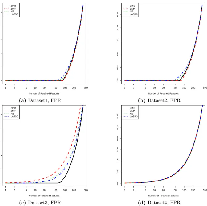
A.3 Comparison of FPR curves between statistical testing and LASSO under four
different zero and count signal situations. . . 36
A.4 Comparison of sensitivity curves between statistical testing and LASSO under
List of Abbreviations
GLMM Generalized Linear Mixed Model
ZINB Zero-Inflated Negative Binomial
ZMP Zero-Modified Poisson
NB Negative Binomial
LASSO Least Absolute Shrinkage and Selection Operator
LRT Likelihood Ratio Test
FDR False Discovery Rate
ROC Receiver Operating Characteristic
FPR False Positive Rate
TPR True Positive Rate
LOOCV Leave-One-Out Cross-Validation
ER Error Rate
1. Introduction
1.1
Background and motivation
The microbiome comprises all of the genetic material within a microbiota (the entire collection of microorganisms in a specific niche, such as the human gut). This can also be referred to
as the metagenome of the microbiota [1]. The far-reaching effects of the microbiome on
human diseases and many other biological phenotypes have only recently discovered [2].
Bacteria in the body and on the surface have a significant impact on the development of health and disease states. For example, microbial changes are shown to be associated with
Parkinson’s disease [3]. The abundance of a bacterium species or genus is quantified by
operational taxonomic unit (OTU) counts using genetic sequence similarity, produced via
targeted amplification and sequencing of the 16S rRNA gene [4].
Microbiome OTU count data often have excessive zeros than what is expected in Poisson or NB models. There are three different types of zeros in Microbiome Data, which are outlier
zeros, structural zeros and sampling zeros [5]. One source of the zero microbiota abundance
is that only a few major bacterial taxa of the microbiota are shared across samples and the rest are detected only in a small percentage of the samples. The zero counts may also be observed when the counts are present with a low frequency but not observed because of sampling variation (sampling zeros). When OTU counts are non-zero, it is often observed that they are highly skewed to the right, often called over-dispersion. There are other statistical issues due to the study designs commonly used in microbiome studies. Microbiome studies usually collect samples with complicated grouping structure, for example, plants from the same plot, and individuals from the same family. The grouping structure in the sample causes correlation among the samples and thus further complicate the analysis and interpretation of microbiome count data. Ignoring the correlation among samples can result in biased inference
and misleading results [6]. Generalized linear mixed effects models are often adopted to
Sample/random variables represent sample collection identifiers in the hierarchical study design, such as family structure, repeated measures from multiple body sites or time points. There is increasing interest among scientists to find the association between the abun-dances of a subset of OTUs and host factors, for example, health disorder, and plant traits;
see [8–10]. For example, [11] reports various relationships between the gut microbiome and
cancer, inflammatory bowel disease (IBD), and obesity. We will call this goal of data analysis by feature selection, that is, to select features related to a response variable. For microbiome data, the features are OTU variables, and the response is a phenotype variable such as disease indicator or plant traits. Currently, researchers fit each OTU variable with gener-alized mixed effect models given the phenotype variable and other factors and then apply a statistical testing method to each OTU to test whether the OTU is differentiated by the
phenotype variable [6, 7]. Features selection can be achieved by thresholding the q-values
returned by the statistical testing procedure. However, statistical testing methods have a number of limitations. First, the validity of q-values relies on the correctness of assumed models, which may not hold for real datasets. Second, q-values and p-values only measure statistical significance but not practical significance. Small q-values do not necessarily imply
strong predictivity [12]. However, researchers still try to find the predictors with q-values
method. For example, many SNPs selected by genome-wide association studies are not good
predictors [12–14]. Third, the joint effects of features on a phenotype cannot be measured
in statistical testing methods that look at each feature individually. Many phenotypes are
believed to be related to multiple features [15–17].
1.2
Methodology
Feature selection can also be achieved by predictive analysis with statistical learning
meth-ods. In this thesis, we consider LASSO multinomial logistic regression [18]. LASSO applies
theL1penalty to the coefficients of the logistic regression model of a phenotype variable given
predictor variables derived from OTU measurements. The OTU variables with non-zero co-efficients after the shrinkage will be selected. There also has been a tentative exploration
still very limited. The reason is probably that many researchers think that LASSO logistic regression may have difficulty in handling the zero-inflation in microbiome data. This moti-vated us to investigate the performance of LASSO logistic regression in microbiome data. We conducted an empirical study using synthetic datasets and a real dataset to investigate the feature selection performance of statistical significance testing and LASSO methods. Four synthetic datasets were generated using zero-inflated negative binomial models (ZINB) with varying signal magnitudes on counts and zeros. We chose to generate datasets from ZINB
models because many researchers in microbiome studies have adopted such models; see [6,7].
We applied the likelihood ratio test (LRT) and LASSO logistic regression to select OTUs that are related to a fixed factor (a phenotype). The feature selection performance of LRT and LASSO are compared with the actual false discovery rate (FDR), which can be calculated in synthetic data with the true indicators of whether an OTU is associated with the pheno-type. We also assessed the agreement of actual false discovery rates and the q-values which are estimates of FDR without using the true association indicators. For LASSO, we also assessed the agreement of cross-validatory predictive measures (error rate and average minus log probabilities) and the actual out-of-sample predictive measures which are obtained with the test sample. Out-of-sample forecast is the process of formally evaluating the predictive capabilities of the models developed using test data to see how effective the algorithms are in reproducing data.
1.3
Summary of results
Our studies with synthetic datasets show that the feature selection performance of LASSO is remarkably excellent in zero-inflated data, and is comparable with the likelihood ratio test applied to the true data generating model. The feature selection performance of LASSO is better when the distributions of counts are more differentiated with the phenotype. Besides, the cross-validatory (CV) predictive measures provide honest measures of the predictivity of
features selected by LASSO. LOOCV can choose the best λ in selecting the most predictive
features in microbiome data. Therefore, the CV predictive measures are proper guidance for
performs slightly worse than likelihood ratio test applied to the true data generating model because LASSO model is not the true model for the dataset and LASSO will lose power even when the model is true for a dataset due to the shrinkage for controlling overfitting. By contrast, when wrong models are fitted to a dataset, the differences between the q-values and the actual false discovery rates are huge; hence, q-values are tremendously misleading for choosing cutoffs in selecting features. Our comparison of LASSO and statistical testing meth-ods in the real dataset shows that small q-values do not necessarily imply high predictivity of selected OTUs.
1.4
Organization of the thesis
In Chapter 2, we introduce the feature selection methods by applying the likelihood ratio test to generalized linear mixed effect models (GLMMs), and by fitting LASSO logistic regression models. We also describe the metrics for comparing feature selection and prediction, including the false discovery rate (FDR), error rate and average minus log probabilities (AMLP). In Chapter 3, we describe how to simulate four datasets using zero-inflated negative binomial (ZINB) with varying signal magnitudes on counts and zeros and a real human gut microbiome data. In Chapter 4, we compare the feature selection performance of LASSO and LRT. We also investigate the performance of cross-validation in estimating the out-of-sample predictive accuracy of LASSO. The thesis is concluded in Chapter 5.
2. Methods
2.1
Feature selection in microbiome data
A typical OTU dataset contains measurements of abundance for OTUs, the total reads, a
number of fixed factors and random factors for each sample, as shown by Table 2.1:
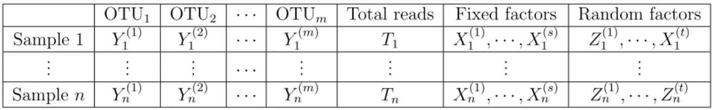
Table 2.1: A general form of microbiome Data
OTU1 OTU2 · · · OTUm Total reads Fixed factors Random factors
Sample 1 Y1(1) Y1(2) · · · Y1(m) T1 X (1) 1 ,· · ·, X (s) 1 Z (1) 1 ,· · ·, X (t) 1 .. . ... ... · · · ... ... ... ... Samplen Yn(1) Yn(2) · · · Yn(m) Tn X (1) n ,· · ·, Xn(s) Zn(1),· · ·, Zn(t)
We will describe the mathematical details of the notations in the Table 2.1:
• Yi(j), i= 1,2, ..., n, j = 1,2, ..., m, is the count number of the OTUj in sample i. This
number can be the abundance of taxa grouped at different levels such as species, genus, and family etc.
• Ti, i= 1,2, ..., n is the total sequence reads for samplei. If we all measured OTUs are
included in our model, Ti =
Pm
j=1Y (j)
i . However, Ti may be smaller than
Pm
j=1Y (j)
i if
some OTUs are omitted for measurement quality control reason.
• Xi(j), i = 1,2, ..., n, j = 1,2, ..., s, represents the jth fixed factor associated for the ith
sample. s is the total number of fixed factors considered in the mixed effect model.
They could be host or clinical factors. When the jth fixed factor is categorical variable
with k classes, Xi(j) is a row vector of k −1 binary variables indicating the class of
sample i.
• Zi(j), i= 1,2, ..., n, j = 1,2, ..., t, represents the jth random factor associated for the ith
sample. t is the number of random factors considered in the mixed effect model. They
group of samples are more similar than the ones from different groups. Random factors
are all categorical. Similar to Xi(j), theZi(j) is a row vector of binary indicator variables
to represent the group identity of sample i in thejth random factor.
An important goal of microbiome studies is to identify/select a subset of OTUs that are
associated/related with a fixed factor, say X(1), which represents a phenotype variable of
interest in real microbiome data, for example, a variable indicating disease status or plant
traits. Currently, researchers fit each OTU variableY(j) with generalized linear mixed effect
models (GLMM) [6] given all fixed and random factors, and then apply a statistical testing
method to test whether the proportion of the jth OTU among all OTUs, often defined as
Yi(j)/Ti, is differentiated (ie, associated) withX(1) [6,7]. Selection of OTUs can be achieved
by thresholding the q-values returned by the statistical testing procedure (likelihood ratio
test). We will describe how to apply likelihood ratio test to GLMMs in Section 2.2 for
selecting OTUs. Statistical learning is another important alternative approach to selecting
OTUs. In LASSO, theX(1) is treated as a response/output variable, and the predictor/input
variables are OTU variables Y(1), . . . , Y(m) after certain transformation, and other fixed and
random factors. Selection of OTUs can be achieved by looking at the coefficients associated with OTU variables. We will describe how to apply LASSO multinomial logistic regression
for microbiome data in Section 2.3.2. The performances of these two distinct methods for
feature selection will be compared with four synthetic data and a real gut microbiome dataset
in Section 4.
2.2
Statistical testing methods
2.2.1
GLMMs for zero-inflated data
Generalized linear mixed model (GLMM) is a flexible modelling framework that can take into account both fixed effects and random effects into the modelling of a response variable. Generalized linear mixed models (GLMMs) are an extension of generalized linear models
(GLMs) [20] and linear mixed models (LMMs) [21]. GLMMs are extended to include both
we will describe three GLMMs which are often used to model count data with zero-inflation
and over-dispersion. We will apply GLMMs to model each OTU variable Yi(j) individually,
conditional on fixed and random factors as shown in Table 2.1. Although different OTUs
are theoretically dependent due to that they are summed to equal to Ti, we adopt this
independent modelling for simplicity by considering that the correlations between OTUs are
very small because the proportion of each OTU is very small whenm is large. For simplicity
in notations, we will omit the OTU index j in Section 2.2.
Negative binomial mixed effect models (NBMM):
For simplicity, we only describe one OTU here without superscriptj. In NBMM, we will
use negative binomial distribution to model Yi given fixed and random factors. The PMF of
Yi is given by: fNB(yi;µi, θ) = Γ(yi+θ) Γ(θ)Γ(yi+ 1) θ θ+µi θ µi θ+µi yi , (2.1)
whereyi takes values in{0,1, . . .},µi >0 is the mean ofyi, andθ > 0 is the inverse dispersion
parameter. In NBMMs, the mean µi is linked to fixed factors and random factors as follows:
log(µi) = log(Ti) +Xiβ+Zib (2.2)
where Xi = (X
(1)
i , . . . , X
(s)
i ) is a vector for representing all fixed factors, and similarly Zi =
(Zi(1), . . . , Zi(t)) is a vector of binary dummy variables for representing all random factors.
The total reads Ti exhibit big differences across samples. Thus, the log of total reads (Ti) is
also considered as a random factor and added to the link function with fixed coefficient 1.
Such a variable is often called an offset variable. In other words, the equation (2.2) links the
log of µi/Ti, i.e., the proportion of the abundance of an OTU among all OTUs, to fixed and
random factors.
The NB distribution has heavier tails than the Poisson distribution. When θ → ∞, the
NB distribution converges to Poisson distribution. Compared to other distributions such as
Poisson or normal, the advantage of using the NB distribution with small parameter θ, such
as 1 or 2, is that the heavier tails of NB can reduce the influence of extraordinarily large
data are the presence of many zeros. To address the zero-inflation in yi, zero-inflated or
zero-modified models have been adopted for modelling yi.
Zero-modified poisson mixed effect model (ZMP):
In zero-modified models [22], also called hurdle models, the probability that yi = 0
is modified be value φi different from what is postulated by a standard distribution such
as the Poisson or NB distributions. The modified probability φi is often linked to fixed and
random factors using logistic regression model. The non-zero values inyi’s, often called count
values, are separately modelled by a zero-truncated distribution, for example, zero-truncated Poisson or NB distribution. Such distributions are often called zero-modified Poisson (ZMP)
or zero-modified NB (ZMNB) models. In particular, the PMF of ZMP for yi is written as:
fZMP(yi) = φi for yi = 0 (1−φi) fPois(y i;µi) 1−fPois(0;µ i) for yi = 1,2, . . . (2.3)
where fPois(yi;µi) denotes the PMF of the Poisson distribution with meanµi. The φi and µi
are often linked to fixed and random factors as follows:
log φi 1−φi = Wiγ+Vir (2.4) log(µi) = log(Ti) +Xiβ+Zib (2.5)
where Xi, Wi, Vi, Zi are covariates constructed from fixed and random factors. Note that the
covariates used in φi and µi are not necessarily the same in theory.
Zero-inflated negative binomial mixed effect models (ZINB)
Another way to model zero-inflated count data is to modelyi as a mixture distribution of
0 and a standard distribution such as Poisson or NB distributions [23], instead of using
zero-truncated distribution for non-zero yi. They are often understood as that theyi is generated
in two steps. The first step is to generate a binary indicator from a logistic regression
distribution. In the second step, if the indicator in the first step is zero, then the yi is zero;
of a zero-inflated negative binomial (ZINB) model for yi can be written as: fZINB(yi) = φi + (1−φi)fNB(0;µi, θ), for yi = 0 (1−φi)fNB(yi;µi, θ), for yi = 1,2, . . . (2.6)
where 0< φi <1 is the probability of an excess zero response. fNB(yi;µi, θ) is the negative
binomial distribution given by (2.1). The parameters µi and φi in ZINB are often linked to
fixed and random factors using the same way as described in equations (2.4) and (2.5).
2.2.2
Likelihood ratio test
In this thesis, we applied likelihood ratio test (LRT) to test whether a fixed factor of interest,
sayX(1), is associated with each OUT variabley(j)
i forj = 1, . . . , mbased on a GLMM model
as described in Section 2.2.1. A vector of p-values p(j), j = 1, . . . , m will be returned from
these tests, and will be converted into q-values q(j), j = 1, . . . , m to reflect false discovery
rate, which will be introduced in Section2.2.3. The OTUs with small false discovery rates
(q-values) will be selected. In this section, we will briefly describe how to apply LRT to GLMM. For more detailed discussion of LRT for testing fixed effects of GLMMs can be found from
[24] and the references therein. We will omit OTU indexj for simplicity. The fixed factor of
interest is denoted by X(1), and all other factors are collectively denoted by X(2). In LRT,
we test the following two model assumptions:
H0 :yi ∼ f(yi|X (2) i ),in words, X (1) i has no effect onyi H1 :yi ∼ f(yi|X (1) i , X (2) i ),in words, X (1) i has effect on yi (2.7)
LetL0 andL1 represent the maximized likelihoods under modelH0 andH1 respectively. The
log likelihood ratio statistic is defined as
Tn= 2(logL1−logL0). (2.8)
If the model H1 is the true model foryi,Tn is expected to be a large value. Therefore, larger
Tn favours H1 against H0. A p-value can be calculated by computing P(Tn > T
(obs)
where Tn(obs) is the observed value of Tn given the dataset. By Wilk’s theorem [25], the
sampling distribution of Tn under H0 is asymptotically a chi-square distribution with degree
freedom α equal to the difference of the numbers of parameters inH0 and H1. Suppose the
number of levels of Xi(1) is K, the degree freedom α is equal to K −1 in NBMM, and α is
equal to 2(K−1) in ZMP and ZINB if Xi(1) is used to model both µi and φi.
2.2.3
False discovery rate and q-value
Due to the large number of OTUs, there is the multiple testing problem. Therefore, we need to convert p-values into false discovery rate to better understand the chance of false positive. Suppose we know the true relationship between OTUs and a phenotype, represented
by a relevancy indicator S(j): S(j) = 1 if the jth OTU is related to the fixed factor X(1)
i
(called alternative hypothesis) and S(j) = 0 if the jth OTU is unrelated to Xi(1) (called
null hypothesis). Given p-values obtained with a statistical test method, we make feature
selection by thresholding p(j) with a cutoff t:
ˆ S(j) = 1 if p(j) ≤t, 0 if p(j)> t. (2.9)
The binary vector, ( ˆS(1), . . . ,Sˆ(m)), is a result of feature selection based on p(j) at cutoff
t. The goodness of ( ˆS(1), . . . ,Sˆ(m)) can be summarized with four numbers: the number of
true positives T P(t) = Pm
j=1I(S
(j)= 1,Sˆ(j) = 1), the number of false positives F P(t) =
Pm
j=1I(S
(j)= 0,Sˆ(j) = 1), the number of true negatives T N(t) =Pm
j=1I(S
(j) = 0,Sˆ(j) = 0),
the number of false negativesF N(t) = Pm
j=1I(S
(j) = 1,Sˆ(j) = 0)), whereI(·) is the indicator
function. We also denote the total number of selected features (rejections of null hypotheses)
by R(t) = F P(t) +T P(t). In terms of p-values, the F P(t) andR(t) are written as follows:
F P(t) = #{p(j)≤t and S(j) = 0;j = 1, ..., m},
R(t) = #{p(j)≤t;j = 1, ..., m}.
(2.10)
Letm0 be the number of OTUs that are unrelated toX
(1)
i , and m1 =m−m0 be the number
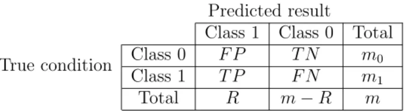
Table 2.2: A feature selection confusion matrix Predicted result
Class 1 Class 0 Total
True condition Class 0 F P T N m0
Class 1 T P F N m1
Total R m−R m
The actual false discovery rate (FDR) of ( ˆS(1), . . . ,Sˆ(m)) is the proportion of false positives
among the selected features:
actual FDR(t) = Number of false positive features
Number of selected features =
F P(t)
R(t) (2.11)
The F P(t), R(t), and actual FDR(t) in (2.11) are random variables. There are many
defi-nitions of a theoretical FDR. [26] defines the positive FDR for independent tests as follows:
FDR(t) =P(S(j) = 0|p(j)≤t)≈ E[F P(t)]
E[R(t)] (2.12)
In practice, we do not know the true relevancy indictorS(j). We need to estimate FDR(t)
with only observed p-values p(j) forj = 1, . . . , m. The observedR(t) is a reasonable estimate
of E[R(t)], which is the number of observed p-values ≤t. Suppose we know the proportion
of unrelated features (null hypotheses) π0 = m0/m. Based on the theory that p-values are
uniformly distributed under null hypothesis (S(j)=0), we can obtain that P( ˆS(j) = 1|S(j) =
0) = P(p(j) ≤ t|S(j) = 0) = t. Then, we can see that E[F P(t)] = m·π
0·t. A conservative
estimate of π0 is 1. This will give an upper bound of FDR(t) as given by [27]. Alternatively,
[28] provides a more accurate estimate by finding a cutoffζ such that the probability density
of p-values are nearly uniform on the right of ζ; the value of this density is expected to be
close to π0. This argument leads to an estimate ofπ0 as follows:
ˆ
π0(ζ) =
#{p(j) ≥ζ;j = 1, ..., m}/m
1−ζ . (2.13)
Given an estimate ˆπ0 for π0, FDR(t) is estimated by
[
FDR(t) = m·πˆ0·t
The q-value for a p-value p(j) is the FDR if we usep(j) as the cutofftin feature selection,
ie, features with p-values ≤ p(j) are selected. To ensure theoretical monotonicity, q(p(j)) is
defined as the minimum of FDR(t) for t≥p(j):
q(p(j)) = min
t≥p(j)
[
FDR(t). (2.15)
If we order all the p-values, and denote thejth p-value byp[j], an approximate for the q-value
is ˆq(p[j]) =m·πˆ
0·p[j]/j, which may not be monotone withp[j], but is easy to calculate and
typically close to q(p[j]) (2.15) whenm is large; see a discussion of FDR by [29].
When the model foryi is correctly specified, the q-values are good estimates of the actual
FDRs, as explained above. In such cases, the q-value is useful guidance for determining the
cutoff t in feature selection. However, in practice, the correctness of a model often lacks
serious verification. Our empirical studies with synthetic datasets will show that there are huge gaps between q-values and actual FDRs when a wrong model (the model describing the data distribution wrongly) is used. This problem is particularly crucial in microbiome data analysis because OTU counts are difficult to model due to the clustering, skewness, and zero-inflation. The basic counts of OTU categories are relative values, which can not be regarded as absolute values. They depend upon the sampling depth corresponding to each sample.
2.3
Predictive analysis with LASSO
2.3.1
Transformation of OTU counts
Statistical learning is another important alternative approach to selecting OTUs. In
statisti-cal learning methods, the phenotype variable Xi(1) is treated as a response/output variable,
and the predictor/input variables are OTU variables Yi(1), . . . , Yi(m) with certain
transforma-tion, and other fixed and random factors. In microbiome data, it is often believed that the phenotype affects the composition of OTUs, rather than the raw counts of OTUs which are
also affected by the total read Ti. As such, a reasonable transformation for OTU counts is
those of all OTUs: ˜ Yi(j) = arcsin q Yi(j)/Ti , for j = 1, . . . , m
Other transformations can be investigated too. For example, if we believe that only the
presence or not of certain OTUs is related to the phenotype, we transform Yi(j) by ˜Yi(j) =
I(Yi(j) > 0), although some information would be lost by dichotomizing the raw data. This
binary transformation is useful for eliminating the adverse effect of the over-dispersion in OTU counts. The choices of transformations are guided by the resulting predictive accuracy in the test sample or using cross-validation.
To be consistent with conventional notations for statistical learning models, we will denote
the phenotype variableXi(1) byyi. Theyiis a categorical variable taking values in{1, . . . , K},
where K is the number of levels of Xi(1); this is different from thatXi(1) is represented by a
K−1 binary indicator variables used as a fixed factor of GLMMs described in Section 2.2.1.
The predictor variables are collectively denoted by xi, which includes ˜Y
(j)
i and all other fixed
and random factors (represented by binary indicator variables). The xi will be a column
vector in this section. The first value in xi is “1” for including an intercept. After we fit a
statistical learning model for yi given xi, selection of OTUs can be achieved by looking at
the coefficients associated with the transformed OTU variables ˜Yi(j).
2.3.2
LASSO multinomial logistic regression
The least absolute shrinkage and selection operator (LASSO) [18] adds theL1of the regression
coefficients as a penalty term to the log likelihood function to achieve shrinkage of regression coefficients for avoiding overfitting and for achieving feature selection. Suppose the response
variable yi has K levels, that is, yi takes values in {1,2, ..., K}. The multinomial logistic
regression links the probability of yi =k toxi using the soft-max function as follows:
P(yi =k|xi, β1, . . . , βK) =
exp(βkTxi)
PK
k=1exp(βkTxi)
, for k= 1, . . . , K, (2.16)
where βk is the collection of all regression coefficients related to yi = k, which is a column
by β. Given observations {(yi, xi), i = 1, . . . , n}, and a tuning parameter λ, the
LASSO-penalized negative log likelihood function is
lLASSO(β) =− n X i=1 log(P(yi|xi, β0, β1, . . . , βK)) +λ K X k=1 ||βk||1, (2.17)
where ||βk||1 is the L1 norm of βk, equal to the sum of absolute values in βk (except the
intercept). The LASSO estimate of β is the minimizer of the LASSO-penalized negative log
likelihood function:
ˆ
βLASSO = argmin
β
lLASSO(β). (2.18)
L1 can shrink the coefficients associated with less important predictor variables into exactly
zeros. The OTU variables with non-zero coefficients will be selected. We fit LASSO
multi-nomial logistic regression (MLR) using an R package called glmnet [30]. This package can fit
LASSO MLR efficiently for a series of different λ values. For each value of λ, we can obtain
a binary feature selection vector as follows:
ˆ SLASSO(j) (λ) = 0, if βk(j)= 0 for all k∈ {1, . . . , K}, 1, otherwise. (2.19)
where βk(j) represents the coefficient associated with the jth OTU for modelling P(yi =k).
The degree of coefficient shrinkage, correspondingly the size of selected features, is
con-trolled by the tuning parameter λ. Larger λ enforces greater shrinkage to the coefficients
β, resulting in selecting fewer predictors in xi. Therefore, the role of λ is similar to that
of the cutoff t for thresholding p-values in statistical testing methods. As discussed in
Sec-tion 2.2.3, one method for choosing t in statistical methods is to look at the false discovery
rates or q-values. In a predictive analysis, a straightforward method for choosingλ is to look
at the predictive performance in test samples, which is measured by a certain metric, for
example, the error rate in predicting yi. Cross-validation is a procedure to split the dataset
into artificial training and test sets to obtain out-of-sample predictive metrics. We use the
leave-one-out cross-validation (LOOCV). We fit the LASSO MLR model by holding the ith
comput-ing the predictive probability uscomput-ing logistic regression model (2.16); let ˆPiλ,−i(k|xi) denote
this CV predictive probability of yi = k, for k = 1, . . . , K. The goodness of ˆPλ,
−i
i (k|xi) for
i = 1, . . . , n can be assessed with the actually observed {yi;i = 1, . . . , n}. We will discuss
two predictivity metrics in Section 2.3.3.
2.3.3
Predictive metrics
Let ˆPi(k|xi) be a predictive probability of yi = k for k = 1, . . . K. We can assess the
goodness of ˆP(yi|xi) with actually observed{yi;i= 1, . . . , n}. The first metric iserror rate.
We predictyi by the k with the highest probability: ˆyi = argmaxkPˆi(k|xi). The error rate is
defined as the proportion of wrongly predicted cases:
ER = 1 n n X i=1 I(ˆyi 6=yi). (2.20)
The second metric is defined as the average of minus log predictive probabilities (AMLP)
at the actually observed yi:
AM LP =−1 n n X i=1 log( ˆPi(yi|xi)). (2.21)
AM LP is more sensitive than ER because it measures not only the correctness of a point
estimate ˆyi but also the degree of correctness expressed by ˆPi(yi|xi).
Both of AM LP and ER should be interpreted relatively not absolutely. Let fk be the
observed frequency of yi = k for k = 1, . . . , K. Without including any predictor in xi (call
the null model), the naive predictive probabilities are ˆPi(0)(k) = fk for k = 1, . . . , K. The
actual CV predictive probabilities will estimate fk with the yi removed, but the frequency
without considering yi is very close to fk. Based on these naive predictive probabilities, the
point prediction is that ˆyi(0) = argmaxkfk. for i = 1, . . . , n. That is, we will predict all the
yi’s by the mode of {yi;i= 1, . . . , n}. The ER with ˆP
(0)
i (k) is
which we will call the baseline error rate. A dataset with more unbalanced distribution in yi
is obviously easier to predict. For example, if maxkfk = 0.9, the baseline error rate is 0.1.
For such an easy dataset, an error rate of 0.1 means that the predictivity of xi for yi is low.
By contrast, if the maximum frequency is 0.6, then the baseline error rate is 0.4. For such
a difficult dataset, an error rate of 0.1 indicates that yi can be fairly well predicted by xi.
Similar to R2 used in linear regression, a relative predictivity metric based onER is defined
as the percentage of the reduction of ER fromER(0):
R2ER = ER
(0)−ER
ER(0) . (2.23)
Similarly, plugging ˆPi(0)(k) =fk for all samples into (2.21), we will see thatnfk of terms in
the summation of (2.21) are equal to log(fk). Then, we can obtain the baseline AM LP(0):
AM LP(0) =−
K
X
k=1
fklog(fk). (2.24)
Note that AM LP(0) is the entropy of {f
k;k = 1, . . . , K}, a quantity for measuring the
un-certainty of fk’s. A relative predictivity metric based onAM LP is defined as the percentage
of the reduction of AM LP from AM LP(0):
R2AMLP = AM LP
(0)−AM LP
3. Data
3.1
Synthetic datasets from ZINB
We generated four synthetic datasets with n = 5000 samples, m = 3000 OTUs, and 5
categorical factors from ZINB models with different signal level settings. In ZINB models, the response variable is modelled as a mixture of structural zeros and an NB distribution. The process for generating one dataset can be described as follows:
Step 1: Generate 5 factors, denoted by Xi(f), for f = 1,· · ·,5, which are used as covariates
for generating OTU counts. Each of the five factors is generated uniformly from
integers 1,· · ·, lf, wherelf represents the number of levels ofX(f). In particular, the
factor X(1) has 10 levels, which will be used as a phenotype variable. The total read
Ti is generated from Poisson distribution with mean λ= 30.
Step 2: A signal vector (S(1), . . . , S(m)) is generated from Bernoulli distribution with
param-eter p = 0.03. S(j) = 0 indicates that the jth OTU is related to the factor X(1),
otherwise unrelated.
Step 3: Fori= 1, ..., nandj = 1, ..., m, generate one OTU countYi(j)for the ith sample and
jth OTU as follows.
Step 3.1: Generate a binary variable Hi(j) to indicate that Yi(j) is a structural zero
or not. The probability of Hi(j) = 0, denoted by φ(ij), is linked to the five
factors using logistic link function:
log φ (j) i 1−φ(ij) ! =γ0+X (1) i γ (1) j +X (2) i γ (2) j +X (3) i γ (3) j +X (4) i γ (4) j +X (5) i γ (5) j
where, γ0 is an intercept; the coefficient vector γ
(f)
j for the factor X(f),
coefficient vectorγj(1) for the phenotype factorX(1) is generated as follows: γj(1) ∼ 0, if S(j)= 0 N(0, σzero2 ) if S(j)= 1
Step 3.2: If Hi(j) = 0, Yi(j) = 0; otherwise, Yi(j) is generated from a NB distribution
with θ= 2 and mean µ(ij), which is linked to the five factors as follows:
log(µ(ij)) = log(Ti) +β0+X (1) i β (1) j +X (2) i β (2) j +X (3) i β (3) j +X (4) i β (4) j +X (5) i β (5) j
where, β0 is an intercept; the coefficient vector β
(f)
j for the factor X(f),
for f = 2,· · ·,5, are generated from a normal distribution N(0,0.22); the
vectorβj(1) for the phenotype factor X(1) is generated as follows:
βj(1) ∼ 0, if S(j) = 0 N(0, σ2 count) if S(j) = 1
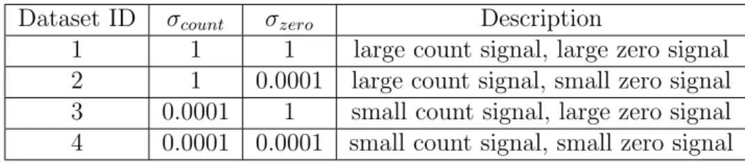
The parameter σzero controls the degree that the status of the jth OTU being zero or
not is affected by the phenotype factor X(1). The parameter σ
count controls the degree that
the magnitude of the count of the jth OTU is affected by the phenotype factor X(1). We will
refer to σzero and σcount respectively as zero signal level and count signal level. These
two parameters are varied at two different levels, resulting in four combinations of zero and
count signal levels. Their values are displayed in Table 3.1. Other parameter settings for the
four datasets are the same.
Table 3.1: Signal level settings for four synthetic datasets.
Dataset ID σcount σzero Description
1 1 1 large count signal, large zero signal
2 1 0.0001 large count signal, small zero signal
3 0.0001 1 small count signal, large zero signal
3.2
A human gut microbiome dataset
We applied the methods described in this thesis to a dataset reported by [10]. The study
cohort contained 1,561 subjects from 2008 to 2014. Fecal samples were collected with 16S
ribosomal DNA sequencing. Their fecal were collected using the stool commode provided by Fisher Scientific. They took an aliquot of stool with a polypropylene specimen collection container. Stool samples were kept frozen until bacterial DNA was extracted. The fecal bacterial DNA was extracted using the QIAamp DNA Stool Mini kit according to the protocol
with minor modifications, including physically disrupting the bacterial cell wall with 0.1−mm
glass beads. Then, non-chimeric sequences were grouped into OTUs at a minimum depth of
30,000 reads/sample with a sequence identity threshold of 97%. They removed the samples
with fewer than 30,000 reads and OTUs with a prevalence of <5% as quality control. The
final data consists of n= 1,098 subjects.
Firmicutes (relative abundance of 64.4 ± 13.9%), Bacteroidetes (26.7 ± 14.8%), and
Actinobacteria (5.0±5.0%) were the three major bacterial phyla. Blautia, Coprococcus,
Ruminococcus, Bacteroides, Dorea, Roseburia, Faecalibacterium, Streptococcus, and Oscil-lospira are found across subjects in the identified 127 genera. The remaining 118 genera were observed irregularly in all subjects.
The study cohort (n = 1,098) consisted of first-degree relatives of Crohn’s disease patients
with asymptomatic self-described white. The average age of the subjects was 20.1±7.8 years
(mean± s.d.; range of 6−35 years). 54.6% were female. We treat the “ethnicity” and “sex”
as fixed effects, “age” as random effects because there are too many levels. We are interested in selecting OTU variables that can predict the ethnicity and quantifying the predictivity of the selected OTUs. The purpose of this analysis is to illustrate the difference between statistical testing and LASSO-MLR methods in selecting features.
4. Results
4.1
Results of analyzing synthetic datasets
In this section, we will investigate the LRT methods applied to three GLMMs (ZINB, ZMP, NB) and LASSO-MLR methods, on the four synthetic datasets generated from a ZINB model,
as described in Section 3.1. We split each dataset into a training dataset with ntrain = 300
subjects and a test dataset with the remaining ntest = 4700 subjects. Only the training
dataset is used to train the GLMMs and LASSO-MLR models. The test dataset is used to check the predictive performance of LASSO-MLR.
In fitting the GLMMs, we treatX(1),X(2)as fixed factors, and the remaining three factors
as random factors. We fit the GLMMs using the R package glmmTMB [31]. In LRT tests, we
use X(1) as a phenotype variable, that is, to test whetherX(1) has an effect on each OTU. A
vector of m= 3000 p-values are calculated for each model and each dataset. We employ the
package glmnet [32] to fit LASSO-MLR models, which use X(1) as a response variable, and
use the remaining four factors and all 3000 transformed OTU variables as predictors. For
the dataset 1 and 2, we transform the OTUs with arcsin(pYij/Ti). For the dataset 3 and 4,
we transform the OTUs with I(Yi(j)>0) since the magnitudes of the OTU counts are nearly
unrelated to the phenotype X(1). For real data analysis, the choice of such a transformation
is guided by cross-validatory or out-of-sample predictive metrics.
For feature selection with LRT p-values, we use all the means between two adjacent
ordered p-values as cutoffs. For each cutoff t, we can obtain a feature selection vector
{Sˆ(j);j = 1, . . . , m} by selecting features with p-values ≤ t. For the synthetic datasets,
the true relevancy indicators {S(j);j = 1, . . . , m} are known. Therefore, we can compute
F P(t), T P(t), R(t), and the actual FDR(t) as described in Section 2.2.3. The left panel of
Figure 4.1 shows the actual FDR(t) against R(t) for each of the three GLMMs; the right
panel of Figure 4.1 shows the ROC curves, ie, T P(t)/(m−m0) against F P(t)/m0. We fit
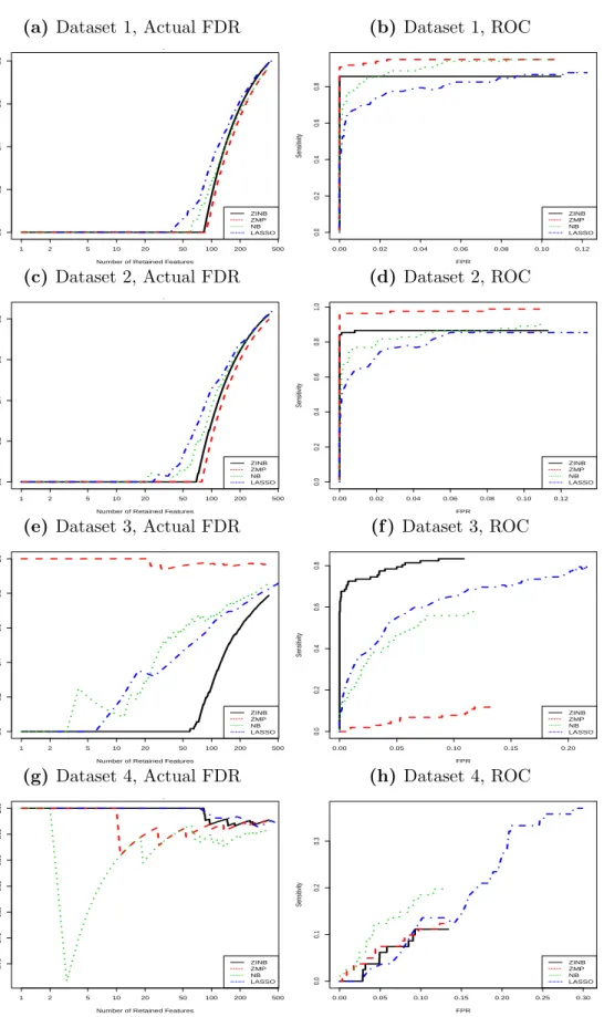
Figure 4.1: Comparison of the actual FDRs of LRT and ROC curves between statis-tical testing and LASSO under four different zero and count signal situations.
(a) Dataset 1, Actual FDR
1 2 5 10 20 50 100 200 500 0.0 0.2 0.4 0.6 0.8
False Discovery Rate
Number of Retained Features
ZINB ZMP NB LASSO (b) Dataset 1, ROC 0.00 0.02 0.04 0.06 0.08 0.10 0.12 0.0 0.2 0.4 0.6 0.8 ROC FPR Sensitivity ZINB ZMP NB LASSO (c) Dataset 2, Actual FDR 1 2 5 10 20 50 100 200 500 0.0 0.2 0.4 0.6 0.8
False Discovery Rate
Number of Retained Features
ZINB ZMP NB LASSO (d) Dataset 2, ROC 0.00 0.02 0.04 0.06 0.08 0.10 0.12 0.0 0.2 0.4 0.6 0.8 1.0 ROC FPR Sensitivity ZINB ZMP NB LASSO
(e) Dataset 3, Actual FDR
1 2 5 10 20 50 100 200 500 0.0 0.2 0.4 0.6 0.8 1.0
False Discovery Rate
Number of Retained Features
ZINB ZMP NB LASSO (f ) Dataset 3, ROC 0.00 0.05 0.10 0.15 0.20 0.0 0.2 0.4 0.6 0.8 ROC FPR Sensitivity ZINB ZMP NB LASSO (g) Dataset 4, Actual FDR 1 2 5 10 20 50 100 200 500 0.70 0.75 0.80 0.85 0.90 0.95 1.00
False Discovery Rate
Number of Retained Features
ZINB ZMP NB LASSO (h) Dataset 4, ROC 0.00 0.05 0.10 0.15 0.20 0.25 0.30 0.0 0.1 0.2 0.3 ROC FPR Sensitivity ZINB ZMP NB LASSO
value of λ, we can use the estimates of the regression coefficients ˆβLASSO to select features
as described in Section 2.3.2, that is, the features with at least one non-zero coefficient are
retained. For each λ, we can compute the number of false positives F P(λ), the number of
true positivesT P(λ), the number of retained featuresR(λ), and the actual FDR(λ) using the
same method described in Section 2.2.3. The plots of FDR(λ) against R(λ) and the ROC
curves ofT P(λ)/(m−m0) againstF P(λ)/m0 are shown in Figure4.1to compare with those
of the LRT methods. From Figure 4.1, we see that, for dataset 1 and 2, LASSO-MLR has
comparable FDRs and areas under the ROC curves with the statistical testing methods; all of the four methods perform similarly; the reason that the LRT tests applied to ZMP appear a little bit better the LRT tests applied to the true model ZINB is that the fittings of ZINB
for a few OTUs that are truly related to X(1) failed to converge. Therefore, The number of
not converging OTUs that are truly related to X(1) in ZINB is less than ZMP model. Hence,
these features were not counted as being selected. For dataset 3, the LRT tests applied to ZINB are better than the other three methods. For dataset 4, all of the four methods do not work well because both of the count and zero signal levels are very small. In summary, the feature selection performances of the LASSO-MLR methods are comparable to those of the statistical testing methods in the synthetic datasets with pretty large count signal levels.
The feature selection performance shown in Figure 4.1 only indicates the goodness of
the orderings of the features in light of their relationships with the phenotype variable. In
practice, we also require a trustable method to determine the threshold (the cutoff t for
p-values and the shrinkage parameter λ for LASSO) for retaining a feature subset. For
statistical testing methods, the choice of t is often guided by the q-values, and for LASSO
the choice of λ is guided by the predictive metrics, for example choosing the λ giving the
best predictive metrics. We will discuss these two issues.
Calculating q-value is a method for estimating actual FDRs given only p-values. The
methods for computing q-values are reviewed in Section 2.2.3. We use the R function
p.adjust from the package stats to convert p-values into q-values. p.adjust has a few
options for computing q-values. We chose the conservative method called “BH” [27]. As
discussed in Section 2.2.3, the BH method estimates the proportion of unrelated OTUs by
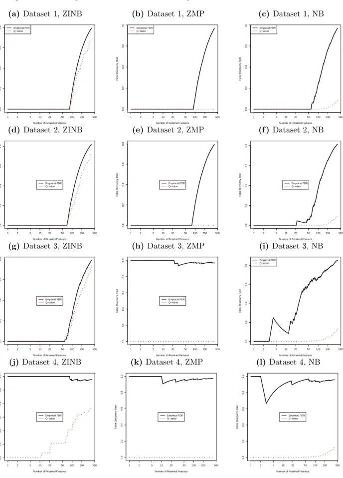
Figure 4.2: Comparison of actual FDRs and q-values for the likelihood ratio tests.
(a) Dataset 1, ZINB
1 2 5 10 20 50 100 200 500 0.0 0.2 0.4 0.6 0.8
False Discovery Rate for ZINB
Number of Retained Features
F alse Disco v er y Rate Empirical FDR Q−value (b) Dataset 1, ZMP 1 2 5 10 20 50 100 200 500 0.0 0.2 0.4 0.6 0.8
False Discovery Rate for ZMP
Number of Retained Features
F alse Disco v er y Rate Empirical FDR Q−value (c) Dataset 1, NB 1 2 5 10 20 50 100 200 500 0.0 0.2 0.4 0.6 0.8
False Discovery Rate for NB
Number of Retained Features
F alse Disco v er y Rate Empirical FDR Q−value (d) Dataset 2, ZINB 1 2 5 10 20 50 100 200 500 0.0 0.2 0.4 0.6 0.8
False Discovery Rate for ZINB
Number of Retained Features
F alse Disco v er y Rate Empirical FDR Q−value (e) Dataset 2, ZMP 1 2 5 10 20 50 100 200 500 0.0 0.2 0.4 0.6 0.8
False Discovery Rate for ZMP
Number of Retained Features
F alse Disco v er y Rate Empirical FDR Q−value (f ) Dataset 2, NB 1 2 5 10 20 50 100 200 500 0.0 0.2 0.4 0.6 0.8
False Discovery Rate for NB
Number of Retained Features
F alse Disco v er y Rate Empirical FDR Q−value (g) Dataset 3, ZINB 1 2 5 10 20 50 100 200 500 0.0 0.2 0.4 0.6 0.8
False Discovery Rate for ZINB
Number of Retained Features
F alse Disco v er y Rate Empirical FDR Q−value (h) Dataset 3, ZMP 1 2 5 10 20 50 100 200 500 0.0 0.2 0.4 0.6 0.8 1.0
False Discovery Rate for ZMP
Number of Retained Features
F alse Disco v er y Rate Empirical FDR Q−value (i) Dataset 3, NB 1 2 5 10 20 50 100 200 500 0.0 0.2 0.4 0.6 0.8
False Discovery Rate for NB
Number of Retained Features
F alse Disco v er y Rate Empirical FDR Q−value (j) Dataset 4, ZINB 1 2 5 10 20 50 100 200 500 0.4 0.5 0.6 0.7 0.8 0.9 1.0
False Discovery Rate for ZINB
Number of Retained Features
F alse Disco v er y Rate Empirical FDR Q−value (k) Dataset 4, ZMP 1 2 5 10 20 50 100 200 500 0.0 0.2 0.4 0.6 0.8 1.0
False Discovery Rate for ZMP
Number of Retained Features
F alse Disco v er y Rate Empirical FDR Q−value (l) Dataset 4, NB 1 2 5 10 20 50 100 200 500 0.0 0.2 0.4 0.6 0.8 1.0
False Discovery Rate for NB
Number of Retained Features
F alse Disco v er y Rate Empirical FDR Q−value
4.2 displays the actual FDRs and q-values against the number of selected features in four datasets. We can see that when the true model (ZINB) is used, the q-values are very close to the actual FDRs. However, when the wrong models (ZMP, NB) are fitted to the datasets, there are huge gaps between the actual FDRs and q-values, and typically the q-values are greatly smaller than the actual FDRs. In particular, for dataset 4 in which the relation-ship between OTUs and the phenotype is very weak, the q-values based on ZMP and NB models are nearly 0 whereas the actual FDRs are nearly 1. These results show that when wrong models are chosen, the resulting q-values are tremendously misleading for choosing the p-value cutoff and the actual FDRs are greatly underestimated.
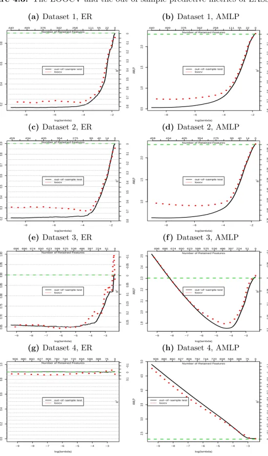
For LASSO-MLR, the choice ofλis guided by predictive metrics. In practice, we can use
LOOCV with only the training dataset to estimate the predictive metrics, which is described
in Section2.3.2. For assessing the performance of LOOCV, we compute the actual predictive
metrics using the test dataset. Figure 4.3 displays the AMLPs, and the ERs obtained with
LOOCV and the test dataset. We see a close matching of the LOOCV and actual out-of-sample predictive metrics. This indicates that LOOCV predictive metrics provide honest measures of the predictivity of the features selected by LASSO. Therefore, the LOOCV
predictive metrics are good guidance for choosing cutoffs (shrinkage parameterλ) in selecting
features.
In addition to guide the choice of λ, the predictive metrics are also good indicators of
the difficulty level in predicting the phenotype with selected OTUs. To demonstrate this, we
show the baseline ERs and AMLPs using green lines in the plots of Figure 4.3, and display
the R2, the percentage of the reduction of ER or AMLP from those in the null model with
no predictor, on the right y-axes. The R2 is a good indicator of the predictivity of selected
features for the phenotype. For example, the maximum R2 values using the optimal λ for
dataset 1 and 2 are larger than those for dataset 3 and 4. Such relative predictive metrics indicate that the phenotype in dataset 1 and 2 is more predictable than the phenotype in
dataset 3 and 4. In particular, the R2 for dataset 4 is near zero, which indicates that there
are very weak relationships between the OTUs and the phenotype. This is the true situation
Figure 4.3: The LOOCV and the out-of-sample predictive metrics of LASSO. (a) Dataset 1, ER −8 −6 −4 −2 0.2 0.4 0.6 0.8 log(lambda) ER f or LASSO ER for LASSO 440 409 376 342 258 111 55 22 0
Number of Retained Features
0.8 0.7 0.6 0.5 0.4 0.3 0.2 0.1 0 R 2 out−of−sample test loocv (b) Dataset 1, AMLP −8 −6 −4 −2 0.5 1.0 1.5 2.0 log(lambda) AMLP
AMLP for LASSO
440 409 376 342 258 111 55 22 0
Number of Retained Features
0.8 0.7 0.6 0.5 0.4 0.3 0.2 0.1 0 R 2 out−of−sample test loocv (c) Dataset 2, ER −8 −6 −4 −2 0.2 0.3 0.4 0.5 0.6 0.7 0.8 0.9 log(lambda) ER f or LASSO ER for LASSO 459 434 405 354 275 99 40 14 0
Number of Retained Features
0.8 0.7 0.6 0.5 0.4 0.3 0.2 0.1 0 R 2 out−of−sample test loocv (d) Dataset 2, AMLP −8 −6 −4 −2 1.0 1.5 2.0 log(lambda) AMLP
AMLP for LASSO
459 434 405 354 275 99 40 14 0
Number of Retained Features
0.75 0.65 0.55 0.45 0.35 0.25 0.15 0.05 0 R 2 out−of−sample test loocv (e) Dataset 3, ER −9 −8 −7 −6 −5 −4 −3 0.65 0.70 0.75 0.80 0.85 0.90 0.95 1.00 log(lambda) ER f or LASSO ER for LASSO 696686 674 650 623 599 575 536486 397 224 51 0 Number of Retained Features
0.25 0.2 0.15 0.1 0.05 0 −0.05 −0.1 R 2 out−of−sample test loocv (f ) Dataset 3, AMLP −9 −8 −7 −6 −5 −4 −3 1.9 2.0 2.1 2.2 2.3 2.4 2.5 log(lambda) AMLP
AMLP for LASSO
696686 674 650 623 599 575 536486 397 224 51 0
Number of Retained Features
0.2 0.15 0.1 0.05 0 −0.05 −0.1 R 2 out−of−sample test loocv (g) Dataset 4, ER −9 −8 −7 −6 −5 −4 −3 0.0 0.2 0.4 0.6 0.8 1.0 log(lambda) ER f or LASSO ER for LASSO 906 880 860 827 806 782 744 720 658 588 388 75 0 Number of Retained Features
0.1 0 −0.1 R 2 out−of−sample test loocv (h) Dataset 4, AMLP −9 −8 −7 −6 −5 −4 −3 2.5 3.0 3.5 4.0 4.5 5.0 log(lambda) AMLP
AMLP for LASSO
906 880 860 827 806 782 744 720 658 588 388 75 0
Number of Retained Features
0 −0.1 −0.2 −0.3 −0.4 −0.5 −0.6 −0.7 −0.8 −0.9 −1 −1.1 R 2 out−of−sample test loocv
4.2
Results of analyzing the gut microbiome data
In this section, we apply the LRT testing methods based on three GLMMs and the
LASSO-MLR method to the human gut microbiome dataset released by [10]. The description of the
dataset is summarized in Section 3.2. The sample size n is 1098. We chose to select OTUs
that can predict the variable ethnicity. The ethnicity has five levels: JewAsh, JewOth,
JewSep, JewUnk and White, with frequencies being 0.096,0.015,0.042,0.011 and 0.836.
There are a total of m = 144 OTUs at genus level. We fit three GLMM models (ZINB,
ZMP, and NB) to each OTU (feature) by considering three covariates, “ethnicity”, “sex” and “age”. We conduct the likelihood ratio test to each OTU to see whether it is affected
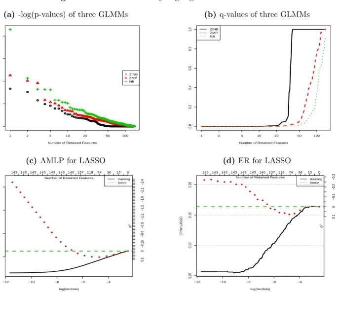
by the ethnicity. The q-values of these three models are shown in Figure 4.4b. We see that
the FDR for the top 20 OTUs is nearly 0. However, the small FDR only indicates that they are related to the ethnicity with a great chance, but does not indicate the strength of the association. The small FDR results from the small p-values, which are probably due to the
large sample size (n = 1098), rather than due to the sharp difference of the proportions of
these OTUs across the five ethnic groups. The predictive analysis looks at how much the ethnicity can be predicted by the OTUs, hence, can quantify the degree of the differentiation of the proportions of the top OTUs across the five ethnic groups. We conducted this analysis
by applying LASSO-MLR to this dataset using LOOCV. Figures 4.4c and 4.4d shows the
error rates and AMLPs for 100 values of λ. The best predictive metrics are reached by a
subset of about 120 (out of 144) OTUs. However, the optimal predictive metrics are very close
to the baseline error rates and AMLPs as shown by the green lines. The R2 for the optimal
error rates and AMLPs are about 20.99% and 16.37% respectively, which indicates that the
predictivity of the 120 OTUs for the ethnicity is pretty low. In summary, the proportions of the top 120 OTUs are indeed differentiated across the five ethnic groups, but the differences are very small. This example shows that the selected features with small q-values may not be highly predictive to a phenotype, or maybe there are other factors we have to measure.
Figure 4.4: Results of analyzing a gut microbiome data.
(a) -log(p-values) of three GLMMs
● ● ● ● ● ●● ● ●● ● ●● ●●●●●●●● ●●●●●●●●●●● ●●●●●●●●●●●●●●●●●●●●●●●●●●●●●●●●●●●●●●●●●●●●●●●●●●●●●●●●●●●●●●●●●●●●●●●●●●●●●●●●●●●●●●●●●●●●●●●●●●●●●●●●●●●●●●●● 1 2 5 10 20 50 100 0 20 40 60 80
−log(p−value) for ZINB, ZMP and NB
Number of Retained Features
●ZINB ZMP NB (b) q-values of three GLMMs 1 2 5 10 20 50 100 0.0 0.2 0.4 0.6 0.8 1.0
q−value for ZINB, ZMP and NB
Number of Retained Features ZINB
ZMP NB
(c) AMLP for LASSO
−12 −10 −8 −6 −4 0.5 1.0 1.5 2.0 log(lambda) AMLP
AMLP for LASSO
143 143 143 143 143 143 140 137 119 74 36 13 0 Number of Retained Features
0.3 0 −0.25 −0.6 −0.9 −1.2 −1.5 −1.8 −2.1 −2.4 R 2 training loocv (d) ER for LASSO −12 −10 −8 −6 −4 0.05 0.10 0.15 0.20 log(lambda) ER f or LASSO ER for LASSO 143 143 143 143 143 143 140 137 119 74 36 13 0 Number of Retained Features
0.1 0 −0.1 −0.2 −0.3 R 2 training loocv
5. Conclusions
In this thesis, we conducted empirical studies using synthetic datasets and a real dataset to investigate the feature selection performance of statistical testing and LASSO methods for zero-inflated microbiome data. Our studies with synthetic datasets show that LASSO is comparable with the likelihood ratio test applied to the true data generating model. It is reasonable that LASSO performs slightly worse than the likelihood ratio test applied to the true data generating model since the multinomial logistic regression model is not the true model for such datasets. However, the performance of LASSO is still remarkable especially when the signals on counts are large enough. The cross-validatory predictive metrics for LASSO provide honest measures of the predictability of the response variable by the features. Therefore, they are useful for choosing reasonable cutoffs in feature selection and are useful to indicate the predictivity of the selected features. On the other hand, for statistical testing methods, when the model is not correctly specified, the q-values (estimated FDR) greatly underestimate the actual false discovery rate. In such cases, the q-values are tremendously misleading for choosing reasonable cutoffs in selecting features. Furthermore, our studies of these two methods in a real dataset show that small q-values do not necessarily imply high predictivity of selected OTUs. In conclusion, if the model is correctly specified, statistical testing methods perform well for selecting features in microbiome data, otherwise incorrect conclusions is likely to be drawn. Therefore, a serious model checking is required when using statistical testing methods. Unfortunately, model checking is rarely conducted in real data analysis. Predictive analysis with LASSO is recommended to supplement statistical testing methods for selecting features and for measuring the predictivity of the selected features.
Bibliography
[1] Samantha A Whiteside, Hassan Razvi, Sumit Dave, Gregor Reid, and Jeremy P Burton.
The microbiome of the urinary tract—a role beyond infection. Nature Reviews Urology,
12:81, jan 2015. URL https://doi.org/10.1038/nrurol.2014.361http://10.0.4.
14/nrurol.2014.361.
[2] Rob Knight, Chris Callewaert, Clarisse Marotz, Embriette R. Hyde, Justine W. Debelius,
Daniel McDonald, and Mitchell L. Sogin. The microbiome and human biology. Annual
Review of Genomics and Human Genetics, 18(1):65–86, 2017.
[3] Timothy R Sampson, Justine W Debelius, Taren Thron, Stefan Janssen, Gauri G Shas-tri, Zehra Esra Ilhan, Collin Challis, Catherine E Schretter, Sandra Rocha, Viviana Gradinaru, et al. Gut microbiota regulate motor deficits and neuroinflammation in a
model of parkinson’s disease. Cell, 167(6):1469–1480, 2016.
[4] Cecilia Noecker, Colin P McNally, Alexander Eng, and Elhanan Borenstein.
High-resolution characterization of the human microbiome. Translational research :
the journal of laboratory and clinical medicine, 179:7–23, jan 2017. ISSN
1878-1810. doi: 10.1016/j.trsl.2016.07.012. URL https://www.ncbi.nlm.nih.gov/pubmed/
27513210https://www.ncbi.nlm.nih.gov/pmc/PMC5164958/.
[5] Abhishek Kaul, Siddhartha Mandal, Ori Davidov, and Shyamal D Peddada. Analysis
of microbiome data in the presence of excess zeros. Frontiers in microbiology, 8:2114,
2017.
[6] Xinyan Zhang, Himel Mallick, Zaixiang Tang, Lei Zhang, Xiangqin Cui, Andrew K
Benson, and Nengjun Yi. Negative binomial mixed models for analyzing
micro-biome count data. BMC Bioinformatics, 18:1–10, 2017. ISSN 1471-2105. doi:
[7] Lizhen Xu, Andrew D. Paterson, Williams Turpin, and Wei Xu. Assessment and
Se-lection of Competing Models for Zero-Inflated Microbiome Data. PLOS ONE, 10(7):
e0129606, July 2015. ISSN 1932-6203. doi: 10.1371/journal.pone.0129606.
[8] W. Duncan Wadsworth, Raffaele Argiento, Michele Guindani, Jessica Galloway-Pena,
Samuel A. Shelburne, and Marina Vannucci. An integrative Bayesian
Dirichlet-multinomial regression model for the analysis of taxonomic abundances in
micro-biome data. BMC Bioinformatics, 18:94, February 2017. ISSN 1471-2105. doi:
10.1186/s12859-017-1516-0.
[9] Keith A. Martinez, Joseph C. Devlin, Corey R. Lacher, Yue Yin, Yi Cai, Jincheng Wang, and Maria G. Dominguez-Bello. Increased weight gain by C-section: Functional
significance of the primordial microbiome. Science Advances, 3(10):eaao1874, October
2017. ISSN 2375-2548. doi: 10.1126/sciadv.aao1874.
[10] Williams Turpin, Osvaldo Espin-Garcia, Wei Xu, Mark S Silverberg, David Kevans, Michelle I Smith, David S Guttman, Anne Griffiths, Remo Panaccione, Anthony Otley, Lizhen Xu, Konstantin Shestopaloff, Gabriel Moreno-Hagelsieb, GEM Project Research Consortium, Andrew D Paterson, and Kenneth Croitoru. Association of host genome
with intestinal microbial composition in a large healthy cohort. Nature Genetics, 48:
1413, October 2016.
[11] Curtis Huttenhower, Dirk Gevers, Rob Knight, Sahar Abubucker, Jonathan H Badger, Asif T Chinwalla, Heather H Creasy, Ashlee M Earl, Michael G FitzGerald, Robert S
Fulton, et al. Structure, function and diversity of the healthy human microbiome.Nature,
486(7402):207, 2012.
[12] Adeline Lo, Herman Chernoff, Tian Zheng, and Shaw-Hwa Lo. Framework for making
better predictions by directly estimating variables’ predictivity. PNAS, page 201616647,
November 2016. ISSN 0027-8424, 1091-6490. doi: 10.1073/pnas.1616647113.
[13] Adeline Lo, Herman Chernoff, Tian Zheng, and Shaw-Hwa Lo. Why significant variables
aren’t automatically good predictors. Proceedings of the National Academy of Sciences,
[14] Klas Gr¨ansbo, Peter Almgren, Marketa Sj¨ogren, J. G. Smith, Gunnar Engstr¨om, Bo Hedblad, and Olle Melander. Chromosome 9p21 genetic variation explains 13%
of cardiovascular disease incidence but does not improve risk prediction. Journal of
internal medicine, 274(3):233–240, 2013.
[15] International Schizophrenia Consortium. Common polygenic variation contributes to
risk of schizophrenia and bipolar disorder. Nature, 460(7256):748, 2009.
[16] Paul DP Pharoah, Antonis Antoniou, Martin Bobrow, Ron L. Zimmern, Douglas F. Easton, and Bruce AJ Ponder. Polygenic susceptibility to breast cancer and implications
for prevention. Nature genetics, 31(1):33, 2002.
[17] Sekar Kathiresan, Cristen J. Willer, Gina M. Peloso, Serkalem Demissie, Kiran Musunuru, Eric E. Schadt, Lee Kaplan, Derrick Bennett, Yun Li, and Toshiko Tanaka.
Common variants at 30 loci contribute to polygenic dyslipidemia. Nature genetics, 41
(1):56, 2009.
[18] Robert Tibshirani. Regression shrinkage and selection via the lasso. Journal of the Royal
Statistical Society. Series B (Methodological), 58:267–288, 1996.
[19] Pixu Shi, Anru Zhang, Hongzhe Li, et al. Regression analysis for microbiome
composi-tional data.