Open source Computational Fluid Dynamics using OpenFOAM

(1)

Open source Computational Fluid Dynamics using

OpenFOAM

H. Medina

1

*, A. Beechook

1

, J. Saul

1

, S. Porter

1

, S. Aleksandrova

1

and S. Benjamin

1 Abstract

Computational Fluid Dynamics (CFD) is a tool that allows designers and engineers to readily evaluate the merits of a given design. It helps reducing the need to build and test prototypes predominantly at the early stages of the design process. CFD has been largely adopted by commercial aircraft manufacturers and is now considered an essential design tool. However, CFD is not as widely used for the design of light aircraft (for example, by amateur or enthusiast designers) mainly due to the cost associated with commercial CFD software. In recent years, a number of open-source CFD initiatives have emerged which have the potential to offer amateur or enthusiast light aircraft designers unrestricted access to CFD technology. In particular, the OpenFOAM project offers one of the most complete open-source CFD solutions and their software can be used without the need to purchase an expensive licence. Nonetheless, there are still some challenges to overcome in order to allow the widespread adoption of the CFD technology OpenFOAM offers by the light aircraft design community. In order to promote the use of OpenFOAM, an introduction of CFD using OpenFOAM (and some complementary open-source tools) will be presented, as well as practical examples and information to allow potential users to overcome some of the common challenges they are most likely to encounter.

Keywords

CFD, OpenFOAM, open source, aerospace, light aircraft, design, porous region

1_{Centre for Mobility and Transport, School of Mechanical, Aerospace and Automotive Engineering, Coventry University, United Kingdom} *Corresponding author: [email protected] or [email protected]

1. Introduction

Computational Fluid Dynamics (CFD) is a tool used to predict the performance of engineering systems or sub-systems on which fluid flow (and other physical mechanisms e.g. heat transfer, combustions, two-phase flows, etc.) plays significant role. Consequently, it is not surprising that CFD is commonly used in a wide range of engineering sectors including the auto-motive, wind energy and aerospace industries. Regardless of the particular industrial application, CFD is used as a design tool to complement (and in some cases ‘replace’) traditional design methodologies involving extensive experimentation and/or prototyping. Despite its limitations1, one of the ad-vantages of incorporating CFD into the engineering design process is that it allows to assess the comparative merits of various design decisions relatively quickly and at a reduced cost (when compared to experimental programmes).

Examples of how CFD is aiding engineering design can be readily found. Della Vecchia et al. [3] used CFD in con-junction with MATLABrto propose an optimised design of a new regional turboprop aircraft configuration for 90 passen-gers. The new design was developed starting from the typical configuration of existing turboprop aircraft for 70 passengers.

1_{Understanding the limitations of CFD is important before it can be}

reliably applied. This is a rather broad topic and it will not be covered in this paper. The interested reader is referred to [1] and [2]

(2)

This example illustrates how CFD can be used to develop new design concepts based on existing, and proven, designs. Furthermore, Della Vecchia’s design resulted in an airframe configuration with improved aerodynamic performance. Boe-lens [4] used thek−ω turbulence model to study the effect

that leading edge geometry features and flap gaps have on the performance of the X-31 aircraft at a range of angles of attack, including post-stall angles of attack. The CFD results were compared with experimental data and, in general, the agreement is shown to be acceptable. Nonetheless, the CFD simulations over-predicted the lift and pitching moment coef-ficients (particularly at higher angles of attack). Panagiotou et al. [5] developed an optimised winglet design for the MALE UAV using CFD. They used the Spallart-Allmaras turbulence model to predict how various winglet designs affected the lift-to-drag ratio characteristics of the UAV. The optimised design led to an increase in endurance of 10%.

In summary, these examples serve to illustrate how CFD is aiding engineers as they seek to develop new designs and/or improve the performance of existing aircraft. Although CFD can now be considered an established design tool and it is routinely employed in aircraft design,CFD is not widely incor-porated into the design of light aircraft (manned), in particular, by amateur and enthusiast light aircraft designers. This trend could be attributed to many factors, which to the knowledge of the authors, have not been investigated and/or identified in the open literature. It could be argued that the cost of commer-cial packages as well as the need to undertake training to be able to confidently apply CFD to light aircraft design may be contributing factors. This paper aims to introduce the funda-mentals of CFD using an open-source package (OpenFOAM) with the purpose to promote the use of CFD for light aircraft design.

2. Brief introduction to CFD

Computational Fluid Dynamics is essentially a method for solving a set of partial differential equations that represent a fluid system. These typically include equations representing the principles of conservation of mass, momentum and en-ergy, as well as auxiliary equations to represent other physical phenomena or sources e.g. porous medium, heat exchangers, actuator discs, magnetic fields, etc. Additional transport equa-tions can also be included within a CFD solution to model the transport of a given property such as species concentration in the case of combustion modelling, or turbulent quantities such as the turbulent kinetic energykand its dissipation rate

εwhen modelling turbulence using the standardk−εmodel.

Therefore, CFD can be used for a wide range of engineer-ing applications provided suitable equations to capture the dominant physics are formulated and implemented into the CFD solver/code. In this section, a brief introduction to the most common techniques for modelling/simulating fluid flow and turbulence are presented, along with relevant and useful sources of further information for the interested reader.

2.1 Modelling approaches

In general, there are three main approaches used to model turbulence: (i) Direct Numerical Simulation (DNS), (ii) Large Eddy Simulation (LES), and (iii) Reynolds Averaged Navier-Stokes (RANS). In DNS, the Navier-Navier-Stokes equations are solved directly (i.e. without the need for a turbulence model) and all the turbulent scales must be captured by the com-putational grid or mesh. Turbulent flows are characterised by a wide range of time- and length-scales. For example, the airflow over an aircraft involves large scales (e.g. wing tip vortices, vortex shedding from the wing, etc.) and small scales (e.g. the flow within the boundary layer or within im-perfections present on the aircraft’s outer structure, such as gaps, steps, waviness, etc.). In DNS, all these structures must be resolved by the grid. Therefore, DNS is the most com-putationally demanding and expensive technique to model turbulence. At present, despite the rapid increase in comput-ing power, DNS is mostly used as a research tool to study flows at low Reynolds numbers (Re=U L/ν) and is not con-sidered a feasible tool for the study of industrially relevant flow configurations or those involving high Reynolds flows.

Another approach used to study turbulence is Large Eddy Simulation (LES). As the name suggests, in LES the large eddies (or turbulent flow structures) are simulated. On the other hand, the small scales (i.e. those that fall within the inertial sub-range) are modelled using sub-grid scale mod-els. The separation of scales is achieved using a spatial filter typically related to the grid size. Therefore, the definition of a ”good” grid for LES is somewhat difficult to specify a priori. However, the separation of scales at the heart of the LES approach leads to a significant reduction in the number of cells needed to carry out a simulation when compared with DNS. Therefore, LES can be used to study industrially rele-vant configurations as it is significantly less computationally demanding than DNS whilst proving a wealth of informa-tion about the dominant flow structures and their temporal evolution. As a result, LES is now generally employed to investigate problems for which the transient features of the flow are important (such as aero-acoustics and combustion applications).

LES is generally too computationally demanding to be used as a design tool during the early stages of the engi-neering design process where typically only top-level per-formance estimations may be required or needed. To this end, the Reynolds-Averaged Navier-Stokes (RANS) approach has been widely used and it has underpinned aircraft de-sign for decades. In RANS, the Navier-Stokes equations are Reynolds-averaged and the flow field is averaged after be-ing decomposed into mean and fluctuatbe-ing components. This process introduces a series of unknown quantities known as the Reynolds stresses which are modelled based on statistical information about the flow. Consequently, RANS models are used to incorporate the effects of turbulence into the solution and provide a means for determining the Reynolds stresses without the calculation of the detailed turbulent flow field.

(3)

Since RANS models are developed based on statistical infor-mation, they are typically fine-tuned for specific applications and there is a very large number of models available. The selection of an appropriate RANS model is one of the chal-lenges faced when applying the RANS approach for engineer-ing design. Additionally, since the Navier-Stokes equations have been averaged to derive the RANS equations, they can only provide solutions or information about the mean flow. However, RANS is orders of magnitude less computationally demanding than DNS and LES, and as a result, it can rapidly provide information about how design decisions may affect the performance of a given design. For this reason, RANS simulations are commonly used in industry despite its obvious limitations.

2.2 CFD workflow

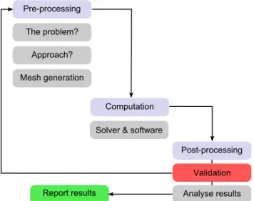
In this section, the typical work flow that is used in CFD will be briefly introduced with the purpose of helping explain the current state-of-the-art (and ease of usage) of open source CFD software (in sections4and5). Figure1illustrates in broad terms the typical steps that a user follows in order to complete a CFD study. AnalyseTresults Post-processing Validation ReportTresults Computation SolverT&Tsoftware MeshTgeneration Approach? TheTproblem? Pre-processing

Figure 1.Typical work flow in CFD

The first, and arguably, the most challenging step is pre-processing. At the stage, the user evaluates the nature and dominant features of the problem and, if possible, makes as-sumptions in order to reduce complexity. Once the dominant physics are identified, the user will select the simulation ap-proach (i.e. DNS, LES or RANS) - typically this choice is made based on computational resource availability. The next stage in the simulation work flow involves the spatial discreti-sation of the simulation domain by building a grid or mesh suitable to the chosen simulation approach (i.e. DNS, LES or RANS). It is worth emphasising that the meshing stage is perhaps the most critical and time consuming step in a typical CFD simulation and the difficulty of generating a ‘good’ mesh

increases with the complexity of the geometry of the problem. Also, the accuracy and validity of the final CFD solution is directly linked to the quality of the underlying mesh employed during the simulation. The final step in the pre-processing stage is to assign appropriate and representative boundary conditions. The choice of boundary conditions will depend on the choice of simulation approach and the physics that will be incorporated into the simulation. For a typical RANS simulation the user must provide suitable boundary conditions for the velocity, the pressure and the turbulence quantities used by the underlying turbulence models e.g.kandεif the

k−εmodel is used (wherekis used to model the turbulent kinetic energy andεmodels its dissipation rate). Ultimately, the choice of boundary conditions is model dependant and the user should gain familiarity with the turbulence model so that appropriate boundary conditions can be used, paying special attention to the requirement/s for wall and inlet boundaries.

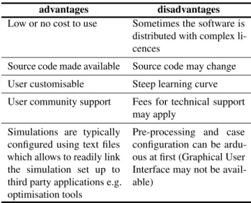
The second phase in the CFD work flow is to carry out the calculations. To achieve this, the user must select an appropriate CFD solver/software/package. This choice can be influenced by various factors such as: software costs, li-censing limitations, ease of use, solvers available, pre- and post-processing tools, software parallelisation, technical sup-port, etc. Another decision the user will face is whether to use open source or commercial (typically without access to the source code) CFD software. Commercial packages have the distinct advantage of being generally well documented and offering technical support to users. However, to benefit from these advantages the cost of utilising commercial packages can be high. On the other hand, open source CFD software may be used at either no cost or at a lower cost when compared with commercial packages and the software developers may or may not offer technical support. This paper aims to pro-mote and highlight the use of open source CFD packages, in particular OpenFOAM, to aid the design of light aircraft and their sub-systems. Nonetheless, there are certain advantages, as well as disadvantages when using open source software (summarised in table1).

The third stage in the work flow involves post-processing (and validation) of the simulations results. Ideally, a validation study should be embedded within the work flow in order to assess the predictive capability of the software, the validity of any assumptions made and the accuracy/applicability of the chosen turbulence model. This stage is essential to be able to gain confidence or to interpret correctly the results produced by the CFD simulation/s. As part of the post-processing phase, the user will typically use the simulation results to calculate quantities of interest2(e.g. aerodynamic coefficients and/or forces) which can be used to assess the merits of a given design or designs. As a result of post-processing, the user may decide to refine the simulation parameters and re-define the pre-processing set up. Alternatively, if the user is satisfied with the results, the findings can be incorporated into the 2_{These are/should be typically selected or identified during the}

(4)

design process (or communicated to others).

advantages disadvantages

Low or no cost to use Sometimes the software is distributed with complex li-cences

Source code made available Source code may change User customisable Steep learning curve User community support Fees for technical support

may apply Simulations are typically

configured using text files which allows to readily link the simulation set up to third party applications e.g. optimisation tools

Pre-processing and case configuration can be ardu-ous at first (Graphical User Interface may not be avail-able)

Table 1.Typical advantages and disadvantages of using open source CFD software

3. Introduction to OpenFOAM

In this section some of the key features that make OpenFOAM a competitive tool for CFD work, as well as a tool suitable for light aircraft design, are introduced. Also in this section, a brief introduction to the structure of a typical OpenFOAM simulation configuration case file is provided. Please note that only a selection of features, utilities and solvers will be discussed. This section is based on the OpenFOAM user guide [6] and it is not meant as a substitute.

3.1 Features overview

OpenFOAM is, in essence, a collection of libraries with func-tionality that allows for these libraries to be used to solve CFD problems. It is based on the finite volume method in which the computational domain is divided (discretised) into small vol-umes and the equations to be solved are re-written to conform to the finite volume approach (the interested reader is referred to Moukalled et al. [7]). At the heart of the OpenFOAM project lies a philosophy of code re-usability, ease of imple-mentation and making the code available to all users to view, review and modify (under the GNU General Public License which ensures that the code remains free and open). As a re-sult of this philosophy, users are allowed to freely modify and contribute to the development of the code (managed by the OpenFOAM Foundation) which has led to an extraordinary rapid pace in its development. For this reason, OpenFOAM is one of the most widely used open source CFD tools available. Also, since OpenFOAM has attracted a large user base with a wide range of scientific/industrial interests, the current default release version (3.0.0) offers users a significant number of fea-tures, ranging from solvers for incompressible and compress-ible flows to conjugate heat transfer, two-phase flows, laminar

flows and turbulence modelling (RANS, LES and DNS), etc. Another interesting feature of the OpenFOAM project is that the development team also offer (commercially) training and support, consultancy and custom code development which has also attracted the interest of industrial users. However, for the academic, amateur or enthusiast user, OpenFOAM offers a platform to perform CFD analysis at no cost, and thanks to a growing user base there is a vibrant user community that can help new users in their discovery of OpenFOAM (e.g. CFD Online [8]). Given the benefits of OpenFOAM outlined above, OpenFOAM has the potential to find a niche user base within the context of aiding individuals and/or organisations with an interest in light aircraft design.

3.2 Useful utilities

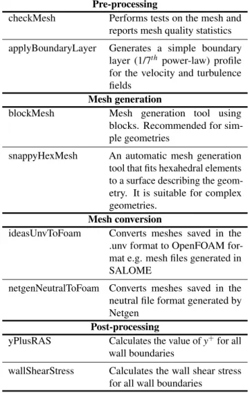
OpenFOAM is released with useful utilities to help the user throughout the entire CFD work flow, from pre-processing, mesh generation, mesh format conversion to post-processing of simulation results. Herein, a summary of utilities that may be of particular interest within the context of light aircraft design are highlighted in table2. It is worth pointing out, in particular for the benefit of new/prospective users, that communication and interaction with OpenFOAM is via the terminal window using written commands i.e. using the name of the executable followed by any options available (that is, the name of utility and/or solver). In order to find out the options available for a particular utility, the user must enter in the command the name of the utility followed by ‘–help’. 3.3 Available fluid solvers

A solver is a computer executable that provides an algorithm to find the solution to a specific set of equations. Although there are many solvers available in OpenFOAM, only incom-pressible solvers will be presented since within the context of light aircraft design the airflow can generally be assumed to be incompressible. A list of the incompressible solvers (excluding incompressible multi-phase solvers) available in OpenFOAM along with a short description of their applicabil-ity is presented in table3.

3.4 Case structure and configuration

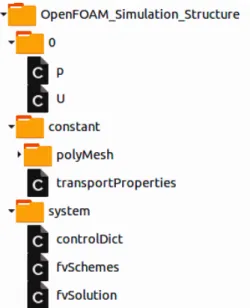
The simulation case structure, set up and configuration of an OpenFOAM simulation is directly linked to the system of equations and domain regions (e.g. fluid or solid regions for conjugate heat transfer problems) used to represent the physical system to be modelled. In this section, for simplicity and relevance, the typical configuration and case structure for modelling incompressible and single-phase problems will be illustrated. The structure of a simulation case in OpenFOAM is shown in figure2. This figure shows the top-level of the simulation folder. Within this folder, three additional directo-ries are required to set up a simulation, namely,0,constant

andsystem. In the0directory the boundary conditions for the simulation are defined and the user must include a series of text files; one for each one of the variables that define the physics of the problem e.g velocity, pressure and turbulence

(5)

Pre-processing

checkMesh Performs tests on the mesh and reports mesh quality statistics applyBoundaryLayer Generates a simple boundary

layer (1/7th power-law) profile for the velocity and turbulence fields

Mesh generation

blockMesh Mesh generation tool using

blocks. Recommended for sim-ple geometries

snappyHexMesh An automatic mesh generation tool that fits hexahedral elements to a surface describing the geom-etry. It is suitable for complex geometries.

Mesh conversion

ideasUnvToFoam Converts meshes saved in the .unv format to OpenFOAM for-mat e.g. mesh files generated in SALOME

netgenNeutralToFoam Converts meshes saved in the neutral file format generated by Netgen

Post-processing

yPlusRAS Calculates the value ofy+for all wall boundaries

wallShearStress Calculates the wall shear stress for all wall boundaries

Table 2.Useful utilities

quantities (such as the turbulent kinetic energy, dissipation rate, transformed eddy viscosity, etc. depending on the turbu-lence model selected by the user). In theconstantdirectory, the software requires entries for aspects of the simulation that remain unchanged through out the simulation e.g. the mesh definition, transport models and turbulence model selection. Also within theconstantfolder, a directory namedpolyMesh

is present in which the mesh information is stored. Note that the majority of the text files required for this folder are au-tomatically generated when a mesh is created or imported. However, theboundaryfile may need to be edited by the user in order to define base boundary types as detailed in the Open-FOAM user guide [6]. Finally, within thesystemfolder, the user defines/controls the simulation by editing at least three text files i.e.controlDict,fvSchemesandfvSolutionwhich are used to control the simulation, define how equations should be discretised and which numerical algorithms should be used to solve the given system of equations.

Solver Description

icoFoam Transient solver for laminar incompress-ible flows. This solver can be applied to low Reynolds applications e.g. internal fluid systems, small UAVs and MAVs simpleFoam Steady state solver for incompressible

flows using the SIMPLE algorithm. It can be used for both laminar and turbu-lent flows (using a background RANS turbulence model)

pisoFoam Transient solver for incompressible flows using the PISO algorithm. It can be used in conjunction with both LES and RANS turbulence models

pimpleFoam Transient solver for incompressible flows using the PIMPLE algorithm (a combination of the PISO and SIMPLE algorithms that allows to maintain nu-merical stability of the simulation whilst using larger time steps). It can be used in conjunction with both LES and RANS turbulence models

Table 3.Incompressible solvers available in OpenFOAM

3.5 Getting started with OpenFOAM

OpenFOAM is natively distributed for Linux operating sys-tems and it can be downloaded on the OpenFOAM Foundation website [9]. There are versions available online that allow OpenFOAM to be installed in Windows, such as the Win-dows version of OpenFOAM distributed by CFD Support [10]. However, Windows versions may not be up to date and may have code bugs that have already been addressed in the Linux version. In regards to the Linux operating system, OpenFOAM provides binary installations for Ubuntu 14.04 LTS and Ubuntu 15.10. Ubuntu is, perhaps, one of the most popular Linux distributions available, and given its large user base, there is a wealth of community support for newcomers. Ultimately, there are other Linux distributions available for prospective OpenFOAM users to choose from (Debian, Open-SUSE, Fedora, Linux Mint, Korora, Mageia, Sparky Linux, Gentoo, etc.) based on their personal preference.

Once the prospective OpenFOAM user has a working ver-sion of Linux and installed OpenFOAM, there are a number of pre-configured incompressible simulation cases located at <installation folder>/OpenFOAM<version>/tutorials /in-compressible. It is recommended to run the ‘cavity’ tutorial first since it is a relatively simple simulation and illustrates the operation of OpenFOAM. To run the tutorial, simply copy the tutorial case anywhere into the localhomedirectory and enter./Allrunin the terminal ensuring that the current working directory corresponds to where the ‘cavity’ tutorial is located (the path of the current working directory can be checked by

(6)

Figure 2.OpenFOAM simulation case structure

enteringpwdin the terminal). Once the user understands the ‘cavity’ tutorial, more complex cases/tutorial can be explored.

Command Description

pwd Display current terminal address cd Change directory e.g. cd /home/User cd .. Change current working path to the

par-ent directory

top Display system processing currently running i.e. similar to the task manager in Windows

ls Display contents at the current level Table 4.Useful Linux terminal commands

4. The challenge of pre-processing

In its own right, pre-processing is challenging since it requires not only an understanding of how a given CFD package oper-ates, but it also requires the user to have a solid understanding of the physics that are present in a given application. Addi-tionally, a crucial step as part of a simulation pre-processing phase is to develop and generate a suitable mesh. Mesh gen-eration, particularly for complex geometries, can be a time consuming activity even when highly specialised commercial grid generation software is used. Furthermore, mesh gener-ation is the main bottleneck for open source CFD because the current state-of-the-art of open source mesh generation tools/software is falling behind commercial products. For example, OpenFOAM offers a very powerful mesh genera-tion tool (snappyHexMesh). AlthoughsnappyHexMeshcan generate high quality grids automatically, its implementation

requires significant amount of RAM memory and, from the us-ability viewpoint, it is difficult to configure it to generate high quality boundary layer grids (inflation layers). Fortunately, there are two reasonable capable open source grid generation tools worth highlighting.

Firstly, the Netgen [11] project provides an algorithm for generating unstructured tetrahedral meshes. It is released with a minimal graphical user interface and it can be used to gener-ate grids for complex geometries. However, Netgen does not offer many features for building CAD geometries. A more complete open source pre-processing solution is provided by SALOME [12] which offers a geometry generation module to build CAD models. Additionally, SALOME includes a mesh generation module capable of producing both hexahedral and tetrahedral meshes, as well as hybrid grids. SALOME can export meshes in .unvformat which include boundary infor-mation and can be easily converted into OpenFOAM format using the ideasUNVtoFoam utility shown in table2. This makes SALOME an ideal open source pre-processor to use in conjunction with OpenFOAM. The main drawback of the SALOME platform is that it uses significant RAM memory when building tetrahedral meshes (since it uses the Netgen algorithm) and, to the authors knowledge, SALOME is not readily parallelised.

The text-based configuration approach used in OpenFOAM can be challenging to new users and involves a steep learning curve. OpenFOAM does not provide a native graphical user interface (GUI). However, engys Ltd. have developed a GUI for OpenFOAM known as HELYX-OS [13] which has been re-leased as open source. It allows to set up and configure Open-FOAM simulations with ease from pre-processing to post-processing of results using ParaView (see section5). HELYX-OS embeds the mesh generation utilitysnappyHexMeshand generates split-hex meshes from a user supplied surface geom-etry files e.g..stlfiles. The graphical interface helps minimise some of the complexity of setting up the snappyHexMesh

utility. It allows to create grids for complex geometries with relative ease and minimal user input. Although HELYX-OS does not support all the features available in OpenFOAM, it is, nonetheless, a useful tool for pre-processing and configuring OpenFOAM simulations which can help new users become familiar with the basic functionality of OpenFOAM.

5. Post-processing and ParaView

Post-processing of OpenFOAM results is facilitated thanks to the ability to export OpenFOAM simulation results to a wide range of third party applications (commercial or open source). The post-processing tools included in OpenFOAM are very powerful and allow sampling of points, lines, planes and surfaces though the simulation domain. The samples can be obtained once the simulation has been completed or during runtime. The utilities that are included in Open-FOAM areprobeLocations and sample which require the definition of a ‘dictionary file’ located within the system

(7)

sam-pling needs of the user. A sample ‘dictionary file’ for these utilities can be found in<installation folder>/OpenFOAM

<version>/applications/utilities /postProcessing /sampling /probeLocations /probesDictand<installation folder> /Open-FOAM<version>/applications/utilities/postProcessing /sam-pling /sample/sampleDict.

Figure 3.Example of the post-processing capabilities of ParaView showing the airflow over an MAV airframe (based on the simulation results from [14])

In addition to the post-processing tools developed by the OpenFOAM team, OpenFOAM is distributed with ParaView [15] which is a versatile post-processing open source software. ParaView has been in constant development since 2000 and is now a tool that rivals commercial packages. It can read OpenFOAM simulations natively and it offers a wide range of filters and data analysis functionality, ranging from data ex-traction to complex 3D rendering and animation. For example, the post-processing of the flow over a Micro-Aerial Vehicle (MAV) shown in figure3was prepared using ParaView and the simulation results presented in [14]. In summary, ParaView is essentially capable of accommodating the post-processing needs of most users.

6. Examples of CFD with OpenFOAM

In this section three examples to showcase the predictive ca-pabilities of OpenFOAM are presented, including (i) Skin friction predictions over a flat plate at zero pressure gradient, (ii) Flow through a 1D porous medium, and (iii) Flow through a planar diffuser with downstream resistance. For succinct-ness, the results are presented avoiding unnecessary detail. The simulation set up and configuration parameters (including boundary conditions) can be found in the original publications referenced in each section.

6.1 Flat plate at zero pressure gradient

OpenFOAM has been used to model the flow over a flat plate at zero pressure gradient using three turbulence models. Re-sults for the predicted skin friction coefficient against the Reynolds number based on the distance from the leading edge (Rex) are shown in figure4. This figure also shows the theo-retical laminar and turbulent skin friction distributions and the experimental results [16] corresponding to a freestream tur-bulence intensity of 3% (ERCOFTAC case T3A). Thek−ω

model [17] is set up in high-Reynolds mode (i.e. it uses

(a)k−ωmodel

(b)Launder-Sharmak−εmodel

(c)k−kL−ωmodel

Figure 4. Skin friction coefficient over a flat plate at zero pres-sure gradient and 3% turbulence intensity. The experimental results corresponding to the T3A case from ERCOFTAC [16]

(8)

Figure 5.Pressure drop though a porous medium (experimental data extracted from [21])

wall functions). As expected, the skin friction distribution follows the theoretical turbulent profile (figure4a) since the wall-function model is based on the logarithmic law of the wall for a turbulent boundary layer at zero pressure gradi-ent. Figure4b shows the results for the Launder-Sharma [18] low-Reynolds model (i.e. it uses damping functions to allow integration of the solution to the wall). This model shows an initial laminar skin friction solution with a sudden jump towards the theoretical turbulent boundary layer skin friction value. Finally, figure4cshows the results from the

k−kL−ωmodel [19] following the implementation detailed

in [20]. Thek−kL−ωmodel is a transition model that uses

the concept of the laminar kinetic energy to model stream-wise pre-transitional velocity fluctuations within the boundary layer to control the transition to turbulence. The results ob-tained using this model are in excellent agreement with the experimental results [16] (ERCOFTAC case T3A).

6.2 Pressure drop though a porous medium OpenFOAM offers the flexibility of modelling incompressible flow through porous medium by incorporating the pressure drop due to the porous medium as a source term in the mo-mentum equations. The Darcy-Forchheimer equation is used to model the pressure drop as a source defined as:

Si=− µDi j+ 1 2ρ|Ukk|Fi j Ui (1) When the porous medium is permeable only in one direc-tion equadirec-tion1can be written as:

S=− µD+1 2ρUsF Us (2)

The pressure drop due to a porous medium that is perme-able only in one direction can be characterised experimentally by recoding the pressure drop against the superficial veloc-ity,Us (i.e. the velocity of the flow as it enters the porous

0 0.5 1 1.5 2 2.5 3 3.5 4 0 0.005 0.01 0.015 0.02 0.025 0.03 0.035 0.04 Velocity (m/s) radial distance (m) Experiment Star CCM OpenFOAM

Figure 6.Downstream velocity profile (experimental data extracted from [22] )

medium), and it can be expressed as shown in equation3. Using equations2and3, the relationship forα,β andD,F

can be found (equations4and5).

∆P L =αUs+βU 2 s (3) α = µD (4) β = 1 2ρF (5)

Figure5shows simulations results based on a configura-tion similar to that presented in [21]. Case 1 in figure5shows that when OpenFOAM is configured using equations4and5, as expected, it returns results that closely follow the experi-mental correlation used. This demonstrates that OpenFOAM has been correctly implemented to deal with simulations in-volving porous media using the Darcy-Forchheimer model (equation1). Also, this figure shows the sensitivity of the porous medium model (equation1) to changes in the viscous tensorDi j.

6.3 2D diffuser with downstream porosity

In this section, a comparison between the predictions obtained using the commercial CFD package Star CCM+ and Open-FOAM is presented. The mesh used and computational set up is described in [22]. The simulations correspond to a pla-nar diffuser with downstream porosity (permeable only in the streamwise direction). A comparison between the experimen-tal and numerical streamwise velocity component profiles at 40mmdownstream from the porous element is presented in figure6. This figure shows that the porous medium model used (equation1) is, perhaps, too simple for the numerical results to mimic the flow physics. However, figure6also shows that the velocity distributions predictions obtained us-ing Start CCM+ and OpenFOAM are in excellent agreement.

(9)

This suggests that the predictive capabilities of OpenFOAM are similar to the commercial CFD software Star CCM+, at least for the configuration tested.

7. Conclusions

In this paper, the CFD software OpenFOAM is introduced along with other open source software that can be used to sup-port the design of light aircraft through the entire CFD work flow. It has been highlighted that OpenFOAM is a powerful tool which offers an extensive range of features to model fluid flow, from incompressible to compressible flows, as well as multi-phase flows. OpenFOAM is distributed with a large number of models, including laminar and turbulence models within the RANS, LES and DNS simulation/modelling frame-works. Pre-processing has been highlighted as the bottleneck of the CFD workflow, in particular, when using OpenFOAM due to its steep learning curve. However, in order to promote and encourage the use of OpenFOAM for light aircraft de-sign, this paper presented other open-source tools that can be used to reduce the difficulties associated with mesh genera-tion and the configuragenera-tion of OpenFOAM simulagenera-tion cases. SALOME is a useful tool that can aid the geometry and mesh generation process and HELYX-OS can be used to config-ure or set up simulations in OpenFOAM. In regards to post-processing, it has been argued that ParaView (an open source post-processing package compatible with OpenFOAM) will satisfy the need of most users. Finally, the predictive capabili-ties of OpenFOAM are showcased for three test cases: (i) a flat plate at zero pressure gradient, (ii) the one-dimensional flow through a porous medium, and (iii) the flow through a planar diffuser with downstream porosity. For all these cases, OpenFOAM is benchmarked against experimental results and shows a good agreement, therefore, demonstrating the po-tential of OpenFOAM as a design tool that can be readily incorporated into the design of light aircraft.

References

[1] _{J. Blazek.} _{Computational Fluid Dynamics: Principles}

and Applications: Third Edition. 2015.

[2] _{S. Biringen and C.-Y. Chow.}_{An introduction to}

computa-tional fluid mechanics by example. 2011.

[3] _{Pierluigi Della Vecchia and Fabrizio Nicolosi.} Aerody-namic guidelines in the design and optimization of new regional turboprop aircraft.Aerospace Science and Tech-nology, 38:88 – 104, 2014.

[4] _{O.J. Boelens. CFD analysis of the flow around the X-31} aircraft at high angle of attack. Aerospace Science and Technology, 20(1):38 – 51, 2012.

[5] _{P. Panagiotou, P. Kaparos, and K. Yakinthos. Winglet} design and optimization for a MALE UAV using CFD.

Aerospace Science and Technology, 39:190 – 205, 2014.

[6] _{CFD Direct. OpenFOAM user guide.} _{http://cfd.direct/} openfoam/user-guide/, 2015. [Online; accessed 26-October-2015].

[7] _{F. Moukalled, L. Mangani, and M. Darwish.} _The

Fi-nite Volume Method in Computational Fluid Dynamics. Springer International Publishing, 2015.

[8] _{CFD Online.} _{Welcome to CFD Online, serving the} CFD community since 1994.http://www.cfd-online.com/, 2015. [Online; accessed 26-October-2015].

[9] _{OpenFOAM Foundation. OpenFOAM – free open source} CFD. http://www.openfoam.org/, 2015. [Online; ac-cessed 20-October-2015].

[10] _{CFD Support. Home Page.} _{http://www.cfdsupport.com/} index.html, 2015. [Online; accessed 27-October-2015]. [11] _{J. Schoberl. Netgen Mesh Generator.} _{http://sourceforge.}

net/projects/netgen-mesher/, 2015. [Online; accessed 22-October-2015].

[12] _{Open Cascade. SALOME.} _{http://www.salome-platform.} org/, 2015. [Online; accessed 27-October-2015]. [13] _{engys. HELYX-OS.} _{http://engys.com/products/helyx-os}_,

2015. [Online; accessed 27-October-2015].

[14] _{N. Madhavan and H. Medina. Pulsed-engine powered} mav: Airframe configurations and wing morphing with cross-winds. Proceedings of the Aerodynamics Confer-ence 2010. Royal Aeronautical Society, July 2010. [15] _{Kitware. ParaView.} _{http://www.paraview.org/}_{, 2015.}

[Online; accessed 27-October-2015].

[16] _{J. Coupland. ERCOFTAC special interest group on} lami-nar to turbulent transition and retransition: T3A and T3B. Technical Report A309514, ERCOFTAC, 1990.

[17] _{D.C. Wilcox. Re-assessment of the scale-determining} equation for advanced turbulence models. AIAA Journal, 26(11):1299–1310, 1988.

[18] _{B.E. Launder and B.I. Sharma. Application of the} energy-dissipation model of turbulence to the calculation of flow near a spinning disc. Letters in Heat and Mass Transfer, 1(2):131–138, 1974.

[19] _{D.K. Walters and D. Cokljat. A three-equation} eddy-viscosity model for reynolds-averaged navier-stokes sim-ulations of transitional flow.Journal of Fluids Engineer-ing, 130(12):1–14, 2008.

[20] _{H. Medina and J. Early. Modelling transition due to} backward-facing steps using the laminar kinetic energy concept.European Journal of Mechanics B/Fluids, 44:60– 68, 2014.

[21] _{S.S. Quadri, S.F. Benjamin, and C.A. Roberts. An} ex-perimental investigation of oblique entry pressure losses in automotive catalytic converters. Proceedings of the Institution of Mechanical Engineers, Part C: Journal of Mechanical Engineering Science, 223(11):2561–2569, 2009.

(10)

[22] _{S. Porter, A. Mat Yamin, S. Aleksandrova, S. Benjamin,} C. A. Roberts, and J. Saul. An assessment of CFD applied to steady flow in a planar diffuser upstream of an auto-motive catalyst monolith.SAE Int. J. Engines, 7(4):1697– 1704, 2014.