Krzysztof Podlaski
Grzegorz Wiatrowski
MULTI-OBJECTIVE OPTIMIZATION
OF VEHICLE ROUTING PROBLEM
USING EVOLUTIONARY ALGORITHM
WITH MEMORY
Abstract The idea of a new evolutionary algorithm with a memory aspect included is proposed to find a multi-objective optimized solution for the vehicle routing problem with time windows. This algorithm uses a population of agents that individually search for optimal solutions. The agent memory incorporates the process of learning from the experience of each individual agent as well as from the experience of the whole population. This algorithm uses crossover operation to define each agent’s evolution. In this paper, we choose the Best Cost Route Crossover (BCRC) operator as a base. This operator is well-suited for VPRTW problems; however, it does not treat both parents symmetrically, which is not natural for general evolutionary processes. A part of the paper is devoted to fin-ding an extension of the BCRC operator in order to improve the inheritance of chromosomes from both parents. Thus, the proposed evolutionary algorithm is implemented with the use of two crossover operators: BCRC and its extended-modified version. We analyze the results obtained from both versions applied to Solomon’s and Gehring & Homberger’s instances. We conclude that the proposed method with the modified version of the BCRC operator gives sta-tistically better results than those obtained using the original BCRC. It seems that an evolutionary algorithm with the memory and modification of the Best Cost Route Crossover Operator leads to very promising results when compared to other solutions presented in the literature.
Keywords vehicle routing problem, time windows, evolutionary algorithms, multi-objective optimization
Citation Computer Science 18(3) 2017: 269–286
1. Introduction
The Vehicle Routing Problem (VRP) is one of the most-recognized of all of the known NP-hard problems in computer science. The problem was proposed by Dantzig and Ramser in 1959’s [6]. Since then, many versions of VRP have been introduced to the literature; e.g., with a time window, truck capacity, trip multiplicity, multi-depots, and other constraints [30]. This paper focuses on the Vehicle Routing Problem with Time Windows (VRPTW).
VRPTW can be described as a task for a single depot with an associated fleet of trucks delivering cargo to many customers with respect to their time constraints. Here are the following rules that must be taken into account during the search for an optimal solution:
•each customer can be visited only once,
•each customer has defined a demand of cargo,
•each customer has defined an opening time window (ready and due time),
•each customer has defined a service time,
•the time of travel between customers is equal to the distance,
•each truck has defined a capacity and has to deliver supplies to customers within the defined time windows,
•a vehicle that arrives too early to a customer has to wait until service would start at the open time for a given customer,
•the customer cannot be serviced if a vehicle arrives after the due time.
Many different approaches to solve VRP have already been proposed: exact [8,12, 31], tabu search [5, 20], heuristic [1, 14], genetic algorithms [2–4, 19, 21, 29], and swarm intelligence [9, 17, 23, 29]. In order to be able to compare the numerical results of dif-ferent methods, some classified benchmark tasks were defined. The best-known ben-chmarks are known as Solomon’s benben-chmarks [27] and Gehring and Homberger’s [10]. The complexity of VRPTW problems makes all approaches that use the exact methods computationally difficult. For large instances with 100 customers or more, it is rarely possible to obtain an optimal route in a reasonable amount time [16]. Moreover, none of existing exact methods can optimally solve all VRPTW benchmark instances with at least 100 customers. For these reasons, the meta-heuristic methods seems to be a better choice for these types of problems.
In this paper, we present an evolutionary algorithm with memory that can be used to solve VRPTW problems. The algorithm uses a population of agents to search for an optimal solution for a given task; each agent stores an actual solution and, additionally, keeps the best historical results already obtained in its memory. The actual solution is the position of an agent in the search space of a VRPTW problem, and an agent movement in this space is obtained due to agent evolution. During the exploration and exploitation processes, the agents evolve and search for better solutions; the new solutions for an agent are created on the basis of its actual solution and historical information gathered using crossover operations. This approach has
been applied to the known benchmarks. After the first numerical experiments, we have discovered that the used crossover operator (Best Cost Route Crossover Operator BCRC) can be modified in order to obtain better results. The mentioned modification is also presented in this paper. The experimental results presented in this paper are interesting and comparable with best-known results from the literature.
The article is organized as follows. Section 2 describes how the aspect of me-mory can be introduced into the population of agents used in evolutionary algorithm. Section 3 is devoted to the BCRC crossover operator for VRPTW and its modifica-tion. Section 4 summarizes the obtained numerical results, while Section 5 focuses on their statistical analysis. Section 6 concludes the paper.
2. Evolutionary algorithm for VRPTW
Evolutionary Algorithms (EA) are based on the evolution of a population of agents, and this evolution should provide a way to search for at least a near-optimal solution for a given problem. A fitness measure is implemented in order to control the evolution of the population in the right direction. The task is to steer the population to search for the most-optimal solution to a given problem. Usually, Evolutionary Algorithms are connected strictly to Genetic Algorithms (GA), but this is not the only possible case. In this paper, we propose an evolutionary algorithm with the use of its memory designed specifically to solve VRPTW tasks.
The algorithm is based on a population of agents, each of which lives in the space of solutions for a given VRPTW instance. The agent stores information about its actual solution (position in search space); additionally, it remembers the best solution already found by this agent and the best solution found by any member of the population. During the evolution process, an agent changes its actual solution (move in search space). The evolutionary changes of the solution for an agent takes into account its actual solution and the historical data stored (memory effect). The solutions of the VRPTW instance is given by chromosome representation known from the usual GA approaches to VRPTW, and the changes of a solution is implemented using a genetic crossover operator.
2.1. Chromosome representation of VRPTV solution
Solutionsof the VRPTV problem has to contain information about the routes of all vehicles va used in the solution. Each of the vehicles starts and ends at the depot. Then, it services its customers, which means it forms an ordered list of all customers to be visited by a given vehicle.
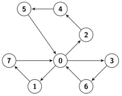
The customers are denoted by an unique integer number (c >0), while the depot is denoted by 0. Each solution is a sequence of serviced customers for all vehicles separated with 0. For example, sequence s in form s = {0,2,4,5,0,1,7,0,3,6,0}
describes a solution of the VRPTW problem that uses three trucks to service seven customers.
The overall length of route s is a sum of the distances covered by all vehicles used in the solution.
|s|=P a|va|, |va|=Pbdist(c b a, cba+1) (1) wherecbadenotes a customer serviced by vehicleva, and functiondist(,)is the distance between two customers. The graphical representation of such a solution is presented in Figure 1. Additionally, solution s has to fulfill all additional constraints, such as truck capacity and the time constraints of the customers.
0 2 4 3 6 5 1 7
Figure 1. Graphical representation of solution s ={0,2,4,5,0,1,7,0,3, 6,0} for VRPTW problem with seven customers and three vehicles.
2.2. Evolution of the population
As mentioned above, we record actual solutionsk and best historical solutionsabk for each member of the population; additionally, we also record the population’s best solution (denoted as spb).
The evolution of thek-th agent is ruled by the following equation:
sk,i=
(
sk,i−1⊗sabk , with probabilityν ab
sk,i−1⊗spb, with probabilityνpb,
(2) where ⊗denotes the crossover operator.
Probabilitiesνab andνpb depend on the overall lengths ofsabk andspb:
νab = |spb| |sab k|+|spb| , νpb = |sabk| |sab k|+|spb| , νab + νpb= 1, (3)
where sk,i is the solution obtained by the k-th agent in the i-th iteration of the al-gorithm. In the presented approach, genetic crossover operator ⊗ is used for the generation of a new solution for an agent and represents a rule that defines the evolu-tion of the agent. There are many available crossover operators in the literature. As the basis for our approach, we have chosen the Best Cost Route Crossover Operator (BCRC) [21].
From (2) and (3), we can observe that, when the historically-best solution found by agent sab
k is much longer than the best solution found by population s pb, the agent prefers to operate with the population’s best solution. Thus, the proposed evolutionary algorithm for the VRPTW problem has the following form.
Algorithm 1 Evolutionary algorithm
1: Begin
2: initialize the population,
3: repeat
4: for allagents in the population,do
5: count new solution of an agent using (2),
6: update an agent best solution if needed,
7: update the population best solution if needed,
8: end for
9: untilthe maximal number of iterations is reached
10: End
11: Algorithm result: return the population best solution as an optimization result.
It is worth mentioning that the evolutionary algorithm for solving problems by searching needs to balance between the exploration and exploitation of the search space [7]. The former is the process of penetrating entirely new regions, while the latter addresses the local search close to the previously found solutions. The presented evolutionary approach incorporates the learning from the experience of each individual agent as well as from the experience of the population (see (2)). In this way, the exploitation process is being incorporated into the method. On the other hand, we will see below that the idea of the modified Best Cost Route Crossover Operator will lead us to the exploration procedure (Sec. 3.2).
2.3. Multi-objectivity and fitness function
In a proposed evolutionary algorithm, very often we have to decide if an actual solution is better than the best from an agent’s historical results or the historically best from the population. For the VRPTW problem (which is a multi-objective optimization problem), we should take into consideration both the number of vehicles involved in the solution as well as the route length of all of these vehicles. Thus, we can distinguish between four different fitness criteria:
•Distance – sum of the distances travelled by the vehicles in the selected solution. The lower the value, the better the solution.
•Distance and Vehicle Count – we try to minimize both of these values, but we set a higher priority on distance.
•Vehicle Count and Distance – similar to the previous criterion, but distance has a lower priority.
•Weighted Method – we try to find the minimum of fitness function F(s) =
α|vs|+β|s|, where|vs|denotes the vehicle count in solutionsand|s|is the dis-tance travelled by the vehicles ins. Parametersαandβ are usually established empirically, and the values are most-often set to: α= 100andβ = 0.001[19, 21].
During our experiments, we decided to use the Weighted Method as the best suited model to represent needs of logistic companies. Analyzing the cost of such types of activities, one can stress that overall distance is connected to the costs of fuel, and the number of vehicles is connected to the costs of the workforce. The choice of the Weighted Method and parametersαandβ express the idea that, for a logistic company, it is better (in economical aspects) to spend a little more on fuel than on an additional truck and driver. On the other hand, we should emphasize that the choice of a fitness policy has an important impact on the final results of the multi-objective decisions.
3. Crossover operators
In the literature, many crossover operators that can be used for combinatorial pro-blems exist; some of them have already been used in VRP [22]. Unfortunately, most of these operators were designed for other combinatorial problems (like TSP), and when applied to VRPTW, one looses’ main information about customers distribution among vehicles in chromosome. This is why such operators enforce the use of additi-onal repair mechanisms in order to obtain a proper VRPTW solution. On the other hand, the Best Cost Route Crossover Operator was designed especially for VRP and does not require any additional repair procedures [21].
3.1. Best Cost Route Crossover Operator
The BCRC recombination operator can be defined as follows. Let us have the chro-mosomes of two parents P1 andP2; we can computeP1⊗P2using algorithm 2. In order to obtain the final result, we should generate two offspring (O12andO21), ex-changing the role of parentsP1andP2in algorithm 2 and choosing the best according to the chosen fitness function.
The presented procedure ensures that, if parents P1 and P2 respect the condi-tions on time and capacity, the obtained offspring also will respect these constraints. A simple example of such a procedure is presented below.
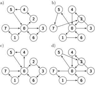
Example BCRC operator(see Fig. 2)
Assume that we have two parents of the following forms:
P1 ={0,2,4,5,0,1,7,0,3,6,0},
P2 ={0,1,6,0,5,7,2,0,3,4,0}.
Suppose that we randomly select vehicle v ={5,7,2} from P2. At the begin-ning, we copy P1into offspringO12and erase fromO12all customers from selected vehiclev; at this point, the offspring would have the following form:
O12 ={0,4,0,1,0,3,6,0}.
Now, we start the procedure of reinserting the missing customers serviced by vehiclevinto offspringO12. We randomly select an element fromv(let us assume that it is customer5) then we find the best place inO12where we can insert this customer.
In the example, the best choice is to insert customer 5 after customer4 serviced by the second car. We have to repeat the same operation for the rest of the elements inv. Algorithm 2 BCRC Crossover
1: Task: Create offspring chromosomeO12.
2: Inputs: parent chromosomesP1,P2, fitness functionf ¯it(x).
3: Begin
4: O12 =P1
5: selectedV ehicle=Rand(P2vehicles.size)
6: candidates=P2vehicles[selectedV ehicle].customers
7: for allcustomer in candidatesdo
8: Erase customer fromO12
9: Update cargo free space for all vehicles inO12
10: end for
11: for allcustomer in candidatesdo
12: min =infinity
13: placeid=−1
14: for allplace in places inO12do
15: TempO=O12
16: insert customer in place to TempO
17: if TempO respects constraintsthen
18: actualLength=f ¯
it(TempO)
19: if actualLength<minthen
20: placeid=place 21: min=actualLength 22: end if 23: end if 24: end for 25: if placeid==−1then
26: add new vehicle with customer toO12
27: else
28: insert customer in placeid intoO12
29: end if
30: end for
31: End
32: Algorithm result: New offspringO12.
At the end, we obtain offspring of the following form (see Figure 2):
O12 ={0,4,5,0,1,7,0,2,3,6,0}
One can observe that most of the edges from parentP1were copied into offspring
O12 and none of edges from parent P2 were copied into offspring O12. A similar procedure is used to create a second offspring (O21). At the end, the best-suited offspring between O12 and O21 is used as a result of the presented recombination procedure. The best-worse relationship for two chromosomes is described in detail in Section 2.3.
a) b) 0 2 4 3 6 5 1 7 0 2 4 3 6 5 1 7 c) d) 0 2 4 3 6 5 1 7 0 2 4 3 6 5 1 7
Figure 2.Graphical representation of BCRC operator example: a) parentP1; b) parentP2; c) offspringO12; d) offspringO21.
3.2. Modification of BCRC operator for VRPTW
The first numerical experiments of the proposed algorithm with the use of the BCRC crossover operator shows that the BCRC operator can be modified in order to obtain better results. The chromosome of the offspring obtained from the application of BCRC on the parent chromosomes shows a similarity to only one of the two parents. This behavior is natural if we analyze the structure of the BCRC operator; the off-spring contains parts copied from only one of the parents, and the other parent only introduces some random mixing. This observation leads to a new Modified BCRC operator that incorporates parts of both of the parents into the offspring chromosome. First, we introduce mean route length dm for vehicle v as an overall length of the route travelled by a vehicle v divided by the number of visited customers. We denote the distance function between customers ca and cb asdist(ca, cb). Assuming that vehicle v visits ncustomers in sequence c1, c2, ..., cn, we can write the formula for mean route length as follows:
dm(v) = dist(0, c1) + hPn−1 i=1 dist(ci, ci+1) i +dist(cn,0) n . (4)
Using the proposed mean route length, we can order all vehicles in a solution from the lowest to the highest values of dm. Then, we denote the vehicle with the lowest mean route length as the best vehicle in the solution and the vehicle with the highest
dm as the worst vehicle in the solution.
The modified BCRC operator applied to parents P1 and P2 is presented in Algorithm 3. As in the case of BCRC, we should have to choose the best from offspring
Algorithm 3 Modified BCRC Crossover
1: Task: Create offspring chromosomeO12.
2: Inputs: parent chromosomesP1,P2, fitness functionf ¯
it(x).
3: Begin
4: for allvehicle inP1vehicles, P2vehiclesdo
5: count value of mean length for vehicle
6: end for
7: identify the vehiclesvb
1, vw1, vb2 andv2w
8: O12 =P1
9: candidates=P1vehicles[vw1]
10: candidates.add(P2vehicles[v2b])
11: selectedV ehicle=Rand(P2vehicles.size)
12: candidates.add(P2vehicles[selectedV ehicle].customers)
13: for allcustomer in candidatesdo
14: Erase customer fromO12
15: Update cargo free space for all vehicles inO12
16: if customer inP2vehicles[v2b]then
17: customers.erase(customer)
18: end if
19: end for
20: O12.vehicles.add(P2vehicles[vb2])
21: for allcustomer in candidatesdo
22: min =infinity
23: placeid=−1
24: for allplace in places inO12do
25: TempO=O12
26: insert customer in place to TempO
27: if TempO respects constraintsthen
28: actualLength=f ¯
it(TempO)
29: if actualLength<minthen
30: placeid=place 31: min=actualLength 32: end if 33: end if 34: end for 35: if placeid==−1then
36: add new vehicle with customer toO12
37: else
38: insert customer in placeid intoO12
39: end if
40: end for
41: End
42: Algorithm result: New offspringO12.
The proposed Modified BCRC operator incorporates elements of chromosomes from both parents and, at the same time, finds the best-possible places for some of the customers (line 21 in 3). An example of such a procedure is presented below.
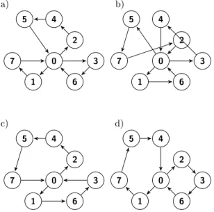
Example Modified BCRC operator(see Fig. 3)
Taking into account the same parents as in the example for BCRC of forms:
P1 ={0,2,4,5,0,1,7,0,3,6,0},
P2 ={0,1,6,0,5,7,2,0,3,4,0}
we can identify the best and worst vehicles in both parents: vb
1={1,7},v1w={2,4,5},
vb1={1,6}, v1w={5,7,2}. At the beginning, we copyP1 into offspringO12and ex-change vehiclevw1 withv2b; thus, it has the following form: O12 ={0,1,6,0,7,0,3,0}.
Suppose that we randomly select vehiclev={3,4}fromP2; in that case, we tempo-rarily haveO12 ={0,1,6,0,7,0}.
Now, we start the procedure of reinserting missing customers 2,3,4,5 into off-springO12. Assuming that we look for the best place for all of the elements in random order 3,4,2,5, we obtain new solutionO12 ={0,1,6,3,0,2,4,7,0}. A similar proce-dure is used to create the second offspringO21(see Fig. 3).
a) b) 0 2 4 3 6 5 1 7 0 2 4 3 6 5 1 7 c) d) 0 2 4 3 6 5 1 7 0 2 4 3 6 5 1 7
Figure 3. Graphical representation of modified BCRC operator example: a) parent P1; b) parentP2; c) offspringO12; d) offspringO21.
4. Experimental results
The presented evolutionary algorithm was implemented with each of the two cross-over operators (BCRC and Modified BCRC). The implementation was applied to the known Solomon’s and Ghering & Homberger’s benchmarks with 50, 100, and 200 cus-tomers. During our experiments, we used a population of30agents. In each algorithm run, we set the maximal number of iterations to 2500. The results presented bellow
suggest that, the bigger the task considered, the more-efficient the results obtained from the Modified BCRC crossover operator are as compared to the original BCRC operator (see Tables 1, 2, and 3).
Table 1
Results for Solomon’s VRPTW benchmark instances with 50 customers. Best means the best result obtained in 100 algorithm runs, Worst is the worst result. Results are presented in the form of #V/#D, where #V is the number of vehicles used and #D is the overall
distance. The best-known results are taken from [11, 13, 15].
Problem
BCRC Modified BCRC Best
known #V/#D
Best Worst Best Worst
#V/#D #V/#D #V/#D #V/#D R101 12/ 13/ 12/ 14/ 12/ 1057.0 1109.8 1058.5 1111.4 1044 [13] R201 4/ 6/ 4/ 7/ 6/ 817.7 873.5 817.7 883.0 791.9 [11] R202 4/ 5/ 4/ 6/ 5/ 729.1 880.4 730.7 825.6 689.5 [11] C101 5/ 6/ 5/ 6/ 5/ 363.2 403.6 363.2 406.8 362.5 [13] C201 3/ 4/ 3/ 4/ 3 361.8 459.5 361.8 469.2 360.2 [15] RC101 8/ 10/ 8/ 10/ 8/ 949.8 1067.4 949.8 1065.4 944 [13] Table 2
Results for Solomon’s VRPTW benchmark instances with 100 customers. Best means the best result obtained in 100 algorithm runs, Worst is the worst result. Results are presented in the form of #V/#D, where #V is the number of vehicles used and #D is the overall
distance. The best-known results are taken from [24, 25, 28].
Problem
BCRC Modified BCRC Best
known #V/#D
Best Worst Best Worst
#V/#D #V/#D #V/#D #V/#D R101 20/ 21/ 19/ 20/ 19/ 1692.6 1758.2 1689.8 1775.8 1650.8 [24] R102 18/ 19/ 17/ 20/ 17/ 1541.4 1581.5 1562.8 1600.7 1486.1 [24] R105 15/ 17/ 15/ 17/ 14/ 1447.4 1582.5 1434.6 1642.7 1377.1 [25] C101 10/ 11/ 10/ 11/ 10/ 828.9 872.4 828.9 869.3 828.9 [24] RC101 15/ 17/ 15/ 18 14 1706.5 1811.2 1684.0 1894.4 1696.9 [28]
Table 3
Results for Ghering & Homberger’s VRPTW benchmark instances with 200 customers. Best means the best result obtained in 100 algorithm runs for each class of instances. Results are presented in the form of #V/#D, where #V is the number of vehicles used and #D is the
overall distance. The best-known results are taken from [26].
Problem BCRC MBCRC Best known [26]
#V/#D #V/#D #V/#D C1 18.9/ 18.9/ 18.9/ 2722.06 2718.48 2718.41 C2 6.0/ 6.0/ 6.0/ 1850.07 1833.25 1831.59 R1 18.2/ 18.2/ 18.2/ 3642.22 3629.17 3611.86 R2 4.0/ 4.0/ 4.0/ 2932.18 2930.12 2929.41 RC1 18.0/ 18.0/ 18.0/ 3185.37 3179.20 3176.23 RC2 4.3/ 4.3/ 4.3/ 2539.52 2537.19 2535.88
The computation times for both of the methods are similar; thus, the better results obtained using Modified BCRC are not due to a longer computation time. In the case of RC101 with 100 customers, our result has a higher number of vehicles and shorter overall distance travelled. However, according to the economic decisions presented in Section 2.3 and the chosen fitness criteria, the best-known solution is still better than the one we obtained. In most of the cases, the number of vehicles for Modified BCRC is optimal; however, the overall distance is only slightly longer than for the best-known solutions.
Our best results are also very similar to the best-known solutions from the lite-rature.In each case, the best-known solution and its reference is given.
5. Statistical comparison of obtained results
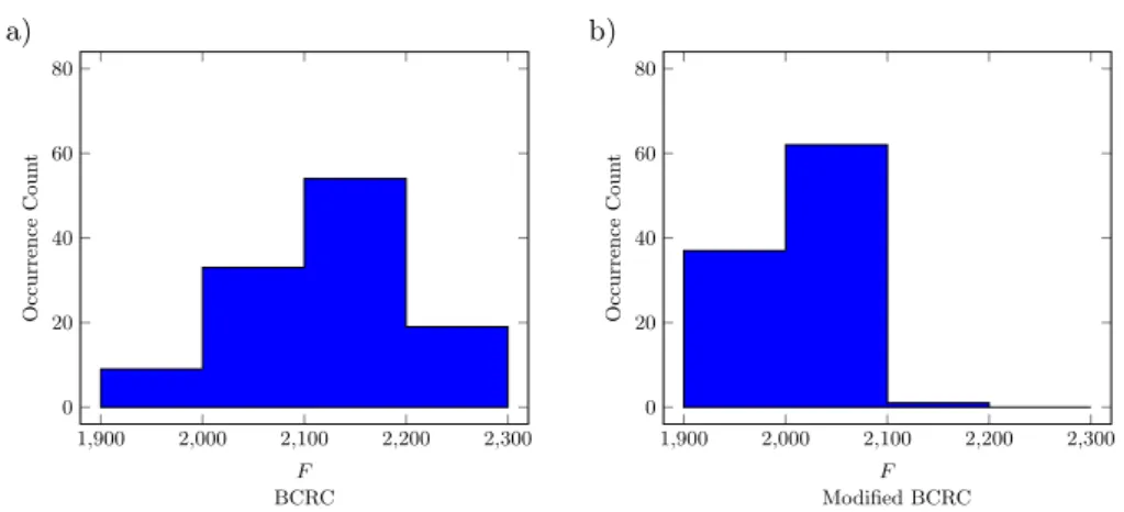
The distribution of results obtained in the numerical experiments suggest that the approach utilizing MBCRC gives better results than that with BCRC (Figs. 4–8). In order to prove this hypothesis, we can use the Mann-Whitney U test [18]. This nonparametric statistical test allows us to decide if two independent statistical samples come from the same population (have the same statistical distribution). The test defines a statistical number calledU based on elements from both samples; the value ofU describes a mixing of results in both samples (for details, see original paper [18], where the construction ofU is defined explicitly). In many cases, the Mann-Whitney U test allows us to prove if one sample represents the population that has statistically larger values than the other.
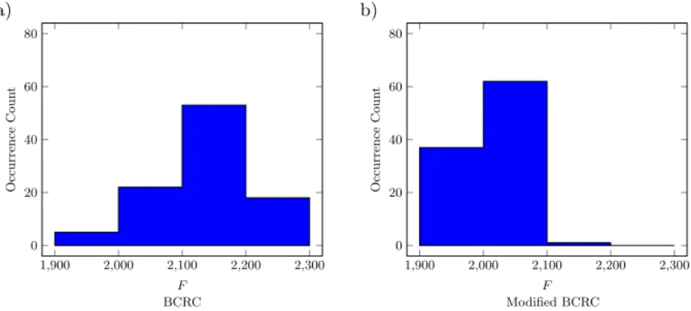
a) b) 1,900 2,000 2,100 2,200 2,300 0 20 40 60 80 F BCRC Occurrence Coun t 1,900 2,000 2,100 2,200 2,300 0 20 40 60 80 F Modified BCRC Occurrence Coun t
Figure 4. Histogram of distribution of the the weighted fitness function (F) values for instance R101 with 100 customers using BCRC (a) and Modified BCRC (b) operators.
F(p) =α|vp|+β|p|, whereα= 100andβ= 0.001.
At first, we have to formulate our null hypothesis (H0) and appropriate alternative hypothesis (H1); then, we apply the Mann-Whitney U test in order to decide if we can accept hypothesisH0.
Hypothesis H0The distributions of the results for both crossover operators BCRC and MBCRC are statistically the same.
Hypothesis H1The distributions of the results for both crossover operators BCRC and MBCRC are statistically different.
a) b) 1,700 1,800 1,900 2,000 2,100 0 20 40 60 80 F BCRC Occurrence Coun t 1,700 1,800 1,900 2,000 2,100 0 20 40 60 80 F Modified BCRC Occurrence Coun t
Figure 5. Histogram of distribution of the the weighted fitness function (F) values for instance R102 with 100 customers using BCRC (a) and Modified BCRC (b) operators.
For each of obtained result distribution, we have calculated statistical value U
and the appropriate zU given by (5):
zu= |U−(n1n2/2)| q n1n2(n1+n2+1) 12 , (5)
where n1, n2 – are sizes of statistical ensembles.
a) b) 2,900 3,000 3,100 3,200 3,300 3,400 0 20 40 60 80 F BCRC Occurrence Coun t 2,900 3,000 3,100 3,200 3,300 3,400 0 20 40 60 80 F Modified BCRC Occurrence Coun t
Figure 6. Histogram of distribution of the the weighted fitness function (F) values for instance R105 with 100 customers using BCRC (a) and Modified BCRC (b) operators.
F(p) =α|vp|+β|p|, whereα= 100andβ= 0.001. a) b) 1,900 2,000 2,100 2,200 2,300 0 20 40 60 80 F BCRC Occurrence Coun t 1,900 2,000 2,100 2,200 2,300 0 20 40 60 80 F Modified BCRC Occurrence Coun t
Figure 7. Histogram of distribution of the the weighted fitness function (F) values for in-stance RC101 with 100 customers using BCRC (a) and Modified BCRC (b) operators.
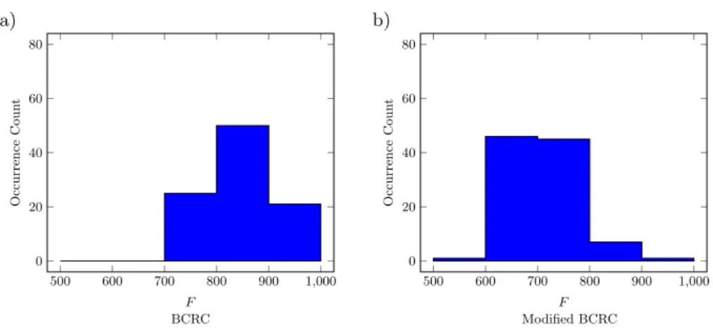
a) b) 500 600 700 800 900 1,000 0 20 40 60 80 F BCRC Occurrence Coun t 500 600 700 800 900 1,000 0 20 40 60 80 F Modified BCRC Occurrence Coun t
Figure 8.Histogram of distribution of the the weighted fitness function (F) for results obtai-ned for instance RC201 with 100 customers using BCRC (a) and Modified BCRC (b)
ope-rators. F(p) =α|vp|+β|p|, whereα= 100andβ= 0.001.
Hypothesis H0 can be accepted with a significance set to 0.05 if zU < 2.575. The results of our statistical tests for instances with 100 customers are presented in Table 4. We can conclude that, for all considered cases, Hypothesis H0 must be rejected.
Table 4
Results of Mann-Whitney U test calculated for distributions of obtained results for instances with 100 customers. Problem U zU R101 963 9.86 R102 137 11.88 R105 43 12.11 RC101 968 9.85 RC201 250 11.60
6. Conclusions
In this paper, we present an evolutionary approach to the vehicle routing problem with time windows. This algorithm uses agents equipped with private and social memory. This is implemented for numerical experiments with two crossover opera-tors: the Best Cost Route Crossover Operator, and its modified version described explicitly in Section 3.2. The original BCRC operator was specially derived for the VRPTW task; the introduction of the presented modification ensures that the parts of chromosomes from both parents can be found in an offspring in contrast to the case with original operator. The results show that, for the analyzed Solomon’s and
Ghering & Homberger’s benchmark tasks, the introduced Modified BCRC operator gives better results than the original one when used in the proposed algorithm for instances with 100 and 200 customers. No mutation operation is included in the presented algorithm due to the conclusion obtained during the preliminary numerical experiments. No significant contribution to algorithm efficiency was observed with mutation applied. Comparing the obtained results with the known optimal results and other presented in the literature, we conclude that the proposed method gives satisfying results statistically better than those obtained using the BCRC operator (Tabs. 3, 4). However, there is still room for improvement; the next modifications of the presented algorithm will be investigated in future works.
References
[1] Battarra M.: Exact and heuristic algorithms for routing problems,4OR, vol. 9(4), pp. 421–424, 2011.http://dx.doi.org/10.1007/s10288-010-0141-9.
[2] Berger J., Barkaoui M.: A parallel hybrid genetic algorithm for the vehicle rou-ting problem with time windows,Computers & Operations Research, vol. 31(12), pp. 2037–2053, 2004.
[3] Braysy O., Gendreau M.: Vehicle Routing Problem with Time Windows, Part I: Route Construction and Local Search Algorithms, Transportation Science, vol. 39(1), pp. 104–118, 2005.http://dx.doi.org/10.1287/trsc.1030.0056. [4] Braysy O., Gendreau M.: Vehicle Routing Problem with Time Windows,
Part II: Metaheuristics, Transportation Science, vol. 39(1), pp. 119–139, 2005.
http://dx.doi.org/10.1287/trsc.1030.0057.
[5] Cordeau J.F., Laporte G., Mercier A.: A unified tabu search heuristic for vehicle routing problems with time windows,Journal of the Operational Research Society, vol. 52(8), pp. 928–936, 2001.
[6] Dantzig G.B., Ramser J.H.: The Truck Dispatching Problem, Management Science, vol. 6(1), pp. 80–91, 1959.
[7] Eiben A.E., Schippers C.A.: On Evolutionary Exploration and Exploitation,
Fundamenta Informaticae, vol. 35(1–4), pp. 35–50, 1998. http://dl.acm.org/ citation.cfm?id=297119.297124.
[8] Fisher M.L.: Optimal Solution of Vehicle Routing Problems Using Minimum K-Trees, Operations Research, vol. 42(4), pp. 626–642, 1994. http://dx.doi. org/10.1287/opre.42.4.626.
[9] Geetha S., Poonthalir G., Vanathi P.T.: A Hybrid Particle Swarm Optimization with Genetic Operator for Vehicle Routing Problem, Journal of Advances in Information Technology, vol. 1(4), 2010.
[10] Gehring H., Homberger J.: A parallel hybrid evolutionary metaheuristic for the vehicle routing problem with time windows. In: Proceedings of EUROGEN99, vol. 2, pp. 57–64, Springer, Berlin, 1999.
[11] Kallehauge B., Larsen J., Madsen O.B.: Lagrangian duality applied to the vehicle routing problem with time windows,Computers &Operations Research, vol. 33(5), pp. 1464–1487, 2006.
[12] Kohl N.: Exact methods for time constrained routing and related scheduling pro-blems. Ph.D. thesis, Technical University of Denmark, 1995.
[13] Kohl N., Desrosiers J., Madsen O.B., Solomon M.M., Soumis F.: 2-path cuts for the vehicle routing problem with time windows, Transportation Science, vol. 33(1), pp. 101–116, 1999.
[14] Laporte G., Gendreau M., Potvin J.Y., Semet F.: Classical and modern heu-ristics for the vehicle routing problem, International Transactions in Operatio-nal Research, vol. 7(4-5), pp. 285–300, 2000. http://dx.doi.org/10.1111/j. 1475-3995.2000.tb00200.x.
[15] Larsen J.: Parallelization of the vehicle routing problem with time windows. Ph.D. thesis, Technical University of Denmark, Danmarks Tekniske Universitet, De-partment of Informatics and Mathematical Modeling, Institut for Informatik og Matematisk Modellering, 1999.
[16] Lenstra J.K., Kan A.: Complexity of vehicle routing and scheduling problems,
Networks, vol. 11(2), pp. 221–227, 1981.
[17] Liu B., Wang L., Jin Y.H.: An effective hybrid PSO-based algorithm for flow shop scheduling with limited buffers, Computers & Operations Research, vol. 35(9), pp. 2791–2806, 2008.
[18] Mann H.B., Whitney D.R.: On a Test of Whether one of Two Random Variables is Stochastically Larger than the Other,The Annals of Mathematical Statistics, vol. 18(1), pp. 50–60, 1947.http://dx.doi.org/10.1214/aoms/1177730491. [19] Minocha B., Tripathi S.: Two Phase Algorithm for Solving VRPTW Problem,
International Journal of Artificial Inteligence and Expert Systems, vol. 4, 2013. [20] Moccia L., Cordeau J.F., Laporte G.: An incremental tabu search heuristic for
the generalized vehicle routing problem with time windows,Journal of the Ope-rational Research Society, vol. 63(2), pp. 232–244, 2012.
[21] Ombuki B., Ross B.J., Hanshar F.: Multi-objective Genetic Algorithms for Vehi-cle Routing Problem with Time Windows, Applied Intelligence, vol. 24(1), pp. 17–30, 2006.
[22] Puljić K., Manger R.: Comparison of eight evolutionary crossover operators for the vehicle routing problem, Mathematical Communications, vol. 18(2), pp. 359–375, 2013.
[23] Reimann M., Doerner K., Hartl R.F.: D-ants: Savings based ants divide and con-quer the vehicle routing problem,Computers &Operations Research, vol. 31(4), pp. 563–591, 2004.
[24] Rochat Y., Taillard É.D.: Probabilistic diversification and intensification in local search for vehicle routing,Journal of Heuristics, vol. 1(1), pp. 147–167, 1995. [25] Shaw P.: Using constraint programming and local search methods to solve vehicle
routing problems. In: Principles and Practice of Constraint Programming – CP98, pp. 417–431. Springer, 1998.
[26] SINTEF: top VRPTW web page. https://www.sintef.no/projectweb/top/ vrptw/.
[27] Solomon M.: Solomon’s VRPTW Benchmark Problems, 1999. http://w.cba. neu.edu/~msolomon/problems.htm.
[28] Taillard É., Badeau P., Gendreau M., Guertin F., Potvin J.Y.: A tabu search heuristic for the vehicle routing problem with soft time windows,Transportation Science, vol. 31(2), pp. 170–186, 1997.
[29] Thangiah S.R., Nygard K.E., Juell P.L.: GIDEON: a genetic algorithm sy-stem for vehicle routing with time windows. In: Proceedings. The Seventh IEEE Conference on Artificial Intelligence Application, vol. i, pp. 322–328, 1991.
http://dx.doi.org/10.1109/CAIA.1991.120888.
[30] Toth P., Vigo D. (eds.): The Vehicle Routing Problem. Society for Industrial and Applied Mathematics, Philadelphia, PA, USA, 2001.
[31] Zhang Z., Qin H., Lim A., Guo S.: Branch and Bound Algorithm for a Single Vehicle Routing Problem with Toll-by-Weight Scheme. In: García-Pedrajas N., Herrera F., Fyfe C., Benítez J., Ali M. (eds.), Trends in Applied Intelligent Sy-stems, Lecture Notes in Computer Science, vol. 6098, pp. 179–188, Springer, Berlin–Heidelberg, 2010. http://dx.doi.org/10.1007/978-3-642-13033-5_ 19.
Affiliations
Krzysztof Podlaski
University of Lodz, Faculty of Physics and Applied Informatics, Łodź, Poland, [email protected]
Grzegorz Wiatrowski
University of Lodz, Faculty of Physics and Applied Informatics, Łodź, Poland, [email protected]
Received: 2.12.2015 Revised: 16.05.2017 Accepted: 20.05.2017