Article Search Tool and Topic Classifier

(1)

ARTICLE SEARCH TOOL AND TOPIC CLASSIFIER

A Thesis by

SANJEEV NARAYANAN

Submitted to the Office of Graduate and Professional Studies of Texas A&M University

in partial fulfillment of the requirements for the degree of MASTER OF SCIENCE

Chair of Committee, Chao Tian Co-Chair of Committee, Anxiao Jiang Committee Members, Tie Liu

Byung-Jun Yoon Head of Department, Miroslav Begovic

December 2019

Major Subject: Electrical Engineering

(2)

ABSTRACT

This thesis focuses on3main tasks related to Document Recommendations. The first approach deals with applying existing techniques on Document Recommendations using Doc2Vec. A robust representation of the same is presented to understand how noise induced in the embedding space affects predictions of the recommendations.

The next phase focuses on improving the above recommendations using a Topic Classifier. A Hierarchical Attention Network is employed for this purpose. In order to increase the accuracy of prediction, this work establishes a relation to embedding size of the words in the article.

In the last phase, model-agnostic Explainable AI (XAI) techniques are implemented to prove the findings in this thesis. XAI techniques are also employed to show how we can fine tune model hyper-parameters for a black-box model.

(3)

DEDICATION

(4)

ACKNOWLEDGMENTS

I use this opportunity to express my gratitude to everyone who supported me throughout this extremely rewarding research experience. I extend my sincere appreciation to my advisor, Dr. Anxiao Jiang for guiding me in every step of this research work.

(5)

CONTRIBUTORS AND FUNDING SOURCES

Contributors

This work was supported by a thesis committee consisting of Professor Chao Tian [advisor], Professor Anxiao Jiang [co-advisor] and Professor Tie Liu & Professor Byung-Jun Yoon of the Department of Electrical and Computer Engineering and

All work conducted for the thesis dissertation was completed by the student independently. Funding Sources

(6)

NOMENCLATURE

BiGRU Bidirectional Gated Recurrent Unit

AI Artificial Intelligence

XAI Hierarchical Attention Network

PDP Partial Dependence Plot

ICE Individual Conditional Expectation

LIME Locally Interpretable Model-agnostic Explanations

SHAP Shapley Additive Explanations

ELI5 Explain Like I’m 5

Doc2Vec Document-to-Vector

Word2Vec Word-to-Vector

RNN Recurrent Neural Network

CNN Convolutional Neural Network

MTC Medical Text Classification

NLP Natural Language Processing

GloVe Global Vectors

LSTM Long-Short Term Memory

(7)

TABLE OF CONTENTS

Page

ABSTRACT . . . ii

DEDICATION . . . iii

ACKNOWLEDGMENTS . . . iv

CONTRIBUTORS AND FUNDING SOURCES . . . v

NOMENCLATURE . . . vi

TABLE OF CONTENTS . . . vii

LIST OF FIGURES . . . ix

LIST OF TABLES. . . xi

1. INTRODUCTION TO TOPICS . . . 1

2. ARTICLE SEARCH TOOL . . . 1

2.1 Motivation and Challenges . . . 1

2.2 Related Work . . . 1

2.2.1 Working of paragraph vectors . . . 3

2.2.2 Document Vectorization. . . 6

2.3 Design - Building a robust search tool . . . 9

2.4 Performance Evaluation . . . 10

3. TOPIC CLASSIFIER . . . 13

3.2 Related Work . . . 13

3.2.1 Attention Network . . . 14

3.2.2 Hierarchical Attention Network . . . 15

3.3 Designs for the Topic Classifier and Integrated Model . . . 17

3.3.1 Experiment 1. . . 17

3.3.2 Experiment 2. . . 17

3.3.3 Experiment 3. . . 17

3.3.4 Experiment 4. . . 18

3.3.4.1 Model Averaging . . . 18

(8)

3.4 Performance Evaluation . . . 20

3.4.1 Results for Experiment 1 . . . 20

3.4.3.1 Query Generation . . . 26

3.4.3.2 Evaluation of the Integrated model . . . 26

3.4.3.3 Discussion . . . 28

3.4.3.4 Why my topic classifier helps in my integrated model . . . 28

3.4.4.1 Model Averaging - Using only fully connected layers . . . 29

3.4.4.2 Model Averaging - Using HAN . . . 29

3.4.4.3 Shallow Learning approach . . . 30

3.5 Applications . . . 30

3.5.1 Medical Text Classifier (MTC) . . . 31

3.5.2 Web of Science Dataset . . . 31

3.5.3 Kaggle Cancer Gene Mutation Dataset . . . 32

4. EXPLAINABLE AI TECHNIQUES . . . 34

4.2 Related Works . . . 34

4.2.1 Complexity related strategy . . . 34

4.2.2 Interpretability via Scoop . . . 35

4.2.2.1 LIME . . . 35

4.2.2.2 SHAP . . . 38

4.2.2.3 ELI5 . . . 44

4.2.3 Model related methods . . . 44

4.3 Designs . . . 46 4.3.1 Experiment 1. . . 46 4.3.2 Experiment 2. . . 46 4.3.3 Experiment 3. . . 46 4.3.4 Experiment 4. . . 46 4.4 Performance Evaluation . . . 47

4.4.1 Result for Experiment 1 . . . 47

4.4.3 Result for Experiment 3 . . . 58

4.4.4 Result for Experiment 4 - Application . . . 60

5. CONCLUSIONS . . . 69

(9)

LIST OF FIGURES

FIGURE Page

2.1 One-hot Encodings . . . 3

2.2 Example of a random encoded vector . . . 4

2.3 Architecture of the neural network [6] . . . 4

2.4 Weights from the example up to hidden layer . . . 5

2.5 Weights from the example up to hidden layer for 3 samples . . . 5

2.6 Output Layer [6] . . . 6

2.7 Comparison of CBOW and document vectors [6] . . . 7

2.8 Flow of document vector generation upto hidden layer . . . 8

2.9 Comparing the drop in Accuracy over the 3 word count ranges . . . 10

2.10 Comparing the drop in Accuracy . . . 11

2.11 Comparing the drop in Accuracy over the 3 word count ranges . . . 12

3.1 Hierarchical Attention Network [22] . . . 16

3.2 Confusion Matrix generated for the test dataset . . . 20

3.3 Training Performance over 7 epochs . . . 21

3.4 A closer look at the model performance in epoch 7 . . . 22

3.5 Embedding Dimension 50, Number of features = 200,000 . . . 22

(10)

3.10 Comparison of Prediction Accuracy of the Integrated model and Doc2vec model

for the 3 datasets . . . 25

3.11 Comparison of Prediction Accuracy of the Model with respect to Threshold for prediction . . . 27

3.12 Single model versus Ensembles . . . 29

3.13 Single model versus Ensembles . . . 30

3.14 Comparison of Embedding dimension variant for the applications. . . 33

4.1 DeepSHAP interpretation [37] . . . 43

4.2 Attention weights for words in every sentence . . . 48

4.3 Attention Output with words that have max attention weights . . . 48

4.4 LIME output . . . 49

4.5 Eli5 output . . . 50

4.6 SHAP summary plot - Class labels correspond to 0: ’Company’, 1: ’Educational Institution’, 2: ’Artist’, 3: ’Athlete’, 4: ’Office Holder’, 5: ’Mean Of Transporta-tion’, 6: ’Building’, 7: ’Natural Place’, 8: ’Village’, 9: ’Animal’, 10: ’Plant’, 11: ’Album’, 12: ’Film’, 13: ’Written Work’ . . . 51

4.7 Explainability per Epoch - MTC dataset . . . 59

4.8 MTC - Output from LIME . . . 61

4.9 MTC - Output from ELI5 . . . 61

4.9 MTC - Output from ELI5 (continued) . . . 62

4.10 MTC - SHAP summary plot - Class 0 - Neoplastic Diseases, Class 1 -Digestive System Diseases, Class 2 -Nervous System Diseases, Class 3 -Cardiovascular Dis-eases and Class 5 -General Pathological Conditions. . . 63

(11)

LIST OF TABLES

TABLE Page

3.1 Cosine similarity score for the top 10 generated documents with and without the

topic classifier . . . 25

3.2 Mean Test performance of commonly used ensemble techniques . . . 30

3.3 MTC - Comparison of the model performance with embedding size . . . 31

3.4 WoS - Comparison of the model performance with embedding size . . . 32

3.5 CGM - Comparison of the model performance with embedding size . . . 32

4.1 Contribution among coalition . . . 38

4.2 Marginal Contribution by different orders . . . 39

4.3 Shapley value for each player . . . 40

4.4 Comparing predicted words over the 4 methods. . . 52

4.5 Comparing the methods for Embedding Dimension - 50 . . . 54

4.9 Score and KL-Divergence values for ELI5 . . . 58

4.10 MTC - Comparing the methods for Embedding Dimension - 50 . . . 64

4.11 MTC - Comparing the methods for Embedding Dimension - 100. . . 65

4.12 MTC - Comparing the methods for Embedding Dimension - 200. . . 66

(12)

1. INTRODUCTION TO TOPICS

The human brain is wired to understand complex sentences and have the ability to draw mul-tiple conclusions from a given statement. Over an individual’s learning period, on an average, a person is exposed to roughly 20,000 to 40,000 different words in English. Along with the knowl-edge of grammar, the number of sentences one can comprehend is unbounded. We are in an era where we focus on automating human tasks to simplify effort. The discipline of Natural Language Processing (NLP) aims to improve the cognitive understanding of texts supplied to the machine. For example, consider a situation where you have read the story of “Snow White and the Seven Dwarves". It so happens that you forgot the names of characters, but you remember the main picture in the story. In order to find the name of the story to fit your flow of thought, you will instinctively Google for all possible phrases that would be coherent with the plot of the story. You may search for the combinations that are not limited to “young girl", “evil queen", “short people", “prince". Your required answer may not even be at the top of your search results. How exactly do we make this more accurate? How will we be able to narrow down our search to the exact answer or in other words, how will a machine be able to provide the result you are expecting? This happens to be a widely researched problem in NLP, which is the crux of my thesis.

Model interpretation at heart, is to find out ways to understand model decision making policies better. This is to enable accountability and transparency which will give users enough credence to use these models in real-world problems which have a lot of impact to business and society. Although, the black-box nature of these systems allow strong predictions, it cannot be precisely explained. AI has already become ubiquitous and we have become reliant on AI making decisions for us in our daily life, from merchandise and movie suggestions on Amazon and Netflix to friend recommendations on Facebook and personalized ads on Google search result pages. Nonetheless, in life-changing inferencing such as disease diagnosis, it is important to know the reasons behind such a critical decision. To address such issues, we use Explainable Artificial Intelligence(XAI) to

(13)

make a transition towards more transparent AI. It aims to create a suite of strategies that produce more explainable models whilst maintaining high performance levels.

(14)

2. ARTICLE SEARCH TOOL

2.1 Motivation and Challenges

We use search and recommender tools mainly for providing personalized suggestion for a task. A good recommender tool understands what a user is looking for. There have been different approaches to this like context based, keyword based or even Collaborative filtering. The main challenge is to build a search tool that is context aware. It tries to derive the overall meaning and big picture behind a search query and not just a local understanding.

2.2 Related Work

Understanding words and deriving meaning from them have been researched since 1980’s. The earliest significant work on word representation started with Brown, et alon bigram and trigram models of predicting the next word(s) given the previous words [1]. The notion “word" by itself was conceived for a machine by Elman , where he explores the correlation between commonly occurring words that form sentences (when sentences are generated at random). He used a net-work with 5 input units, 20 hidden units, 5 output units, and 20 context units to produce a 5-bit representation for the words [2]. When Rumelhart,et alperfected the backpropagation algorithm for neural networks, word representations started to form a much more concrete structure and the tasks for future work started to get more clear [3].

We have now come a long way from bigram and trigram models to learn an n-gram representation. In any case, the straightforward procedures are at their limits in numerous errands. For exam-ple, there are limited amounts of relevant in-domain information for automated speech recognition whose performance is typically controlled by the size of high-quality transcribed speech data (often just millions of words). In machine translation, the existing corpora for numerous dialects contain as it were a couple of billions of words or less. Mikolov ,et algave the idea computing continuous vector representations of words from very large data sets [4]. The quality of these representations

(15)

were measured in a word similarity task. His work on word2vec has been an industry standard in a lot of NLP practices and served as one of the first steps in semantic cognition. It sparked a lot of applications in Information Retreival, Document Classification and many more. Pennington,et al suggested that two words can be better distinguished with respect to a context word by the ratio of the co-occurrence probabilities [5]. This function, that distinguishes two word vectors based on a context word vector need to be formalized in a way that it is symmetric between context words and words. Their model weighs all the co-occurrences equally. This GloVe vector representation has taken the best of the Matrix factorization models and Local context window models and presented a computationally simple yet efficient model to determine a rich distributed word representations.

Text classification and clustering have always played an important role in document retrieval. Such algorithms typically require a fixed-length vector to represent the text input. Le ,et alproposed the idea of a paragraph vector, an unsupervised framework that learns continuous distributed vector representations for pieces of texts [6]. The texts can be of variable-length, ranging from sentences to documents. This technique was inspired from a multiple researches (Bengio,et al[7] , Collobert ,et al[8]) where each word is represented by a vector which is concatenated or averaged with other word vectors in a context, and the resulting vector is used to predict other words in the context. Paragraph vectors attempt to learns features that are relevant to the tasks at hand given very limited prior knowledge.

Over time, learning representations were explored using transfer learning based approaches, graph based approaches and using convolutional neural networks. Koopman, et alused a 2 step approach to improve discriminating ability of the vector representations for document embeddings [9]. They first reduce the dimensionality of the term vectors by an extremely efficient imple-mentation of random projection [10] [11]. They then project the term vectors on the hyperplane orthogonal to the average language vector. Tang,et alstudied the problem of integrating very large

(16)

information networks into low-dimensional vector spaces, which is useful in many tasks such as visualization, classification of nodes and prediction of links [12]. The authors proposed a model that optimizes an objective which preserves both the local and global network structures. In many real world scenarios of graph based embedding algorithms [13] [14] [15], aim to preserve the first-order proximity between the vertices. However, these are seldom sufficient. In the paper, the authors explore a second-order proximity between the vertices, defined not by the observed intensity of the connection, but by the mutual neighborhood structures of the vertices. Peters, et al[16] and Conneau,et al[17] used bi-LSTM based learning representations that model dynamic word-use characteristics and how they vary across various linguistic contexts.

2.2.1 Working of paragraph vectors

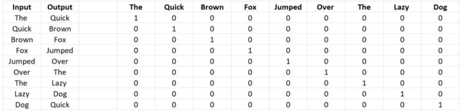
Before we get to paragraph vectors, let us look at continuous Bag-of-words (CBOW) represen-tation. CBOW’s way of working is that it tries to estimate the probability of a word given a context. A context-setting may be a single word or a group of words. Consider the example of this sentence The quick brown fox jumped over the lazy dog. For ease of understanding, let us consider a sliding window of length 1. This corpus can be translated as follows into a training set for a CBOW model

Figure 2.1: One-hot Encodings

In the image below, the matrix on the right represents the one-hot encoded data on the left.

(17)

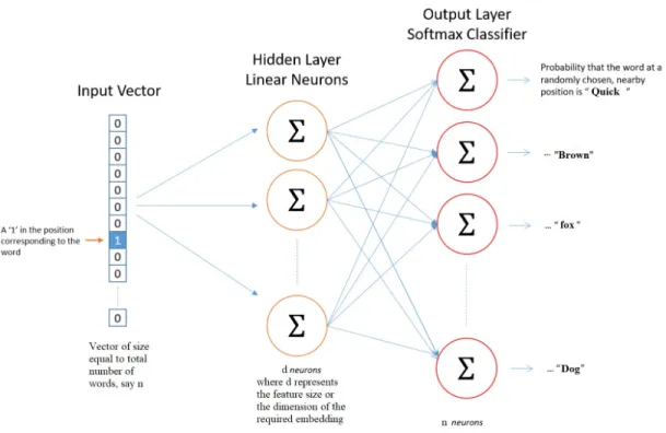
Figure 2.2: Example of a random encoded vector

way to convert this one-hot encoded representation into the word embedding. This matrix dis-played in the above image is sent to a three-layer shallow neural network: an input layer, a hidden layer and an output layer. The output layer is a softmax - used to sum the probabilities obtained in the output layer up to 1. From the Figure 2.2 , We have the encoded vector as the input to this neural network. The hidden layer is a randomly initialized set of numbers that form the feature space of the entire vocabulary. This means, we have an d-dimension vector for every word in the vocabulary. This is equivalent to telling that the hidden layer acts as a look-up table for every word. Let us for example, fixd= 6

(18)

From the above example, this can be represented as :

Figure 2.4: Weights from the example up to hidden layer

The network output is a single vector (also with 6 components) containing the probability of a randomly selected nearby word being that vocabulary word for each word in our vocabulary. Note that the hidden layer neurons do not have an activation function. Now consider the hidden layer. Looking at the rows of this weight matrix, it’s really what our word vectors are going to be. So the ultimate goal of all this is only learning this matrix of hidden layer weight. Extending this example to learning 3 words, we get

Figure 2.5: Weights from the example up to hidden layer for 3 samples

The above picture takes 3 contextual words and estimates a target word’s probability. As shown above in blue, orange and green, the output can be assumed to take three one-hot encoded vectors in the input layer. The measures remain the same, only the calculation of hidden activation changes. Instead of simply copying the input-hidden weight network rows to the output layer, all matrix rows are taken on average. With the above example, we can appreciate this. The output layer is a softmax regression classifier. - output neuron (one per term in the lexicon) yields between 0 and 1,

(19)

and all these output values are summed up to 1.

Next comes the training. The objective function is the negative log likelihood of a word, given its context. Here this likelihood is the softmax output of the network. The gradients are updated by the rule of stochastic gradient descent and we finally learn the weights of the words in our vocab-ulary. While we can train our word vectors based on our corpus, we can also use existing weights that are available online to speed up our training.

Figure 2.6: Output Layer [6]

2.2.2 Document Vectorization

Document Vectorization is an extension to the word vectorization approach towards documents. Its intention is to encode (whole) documents, consisting of lists of sentences, rather than lists of ungrouped sentences. Let us look at some differences to understand an overview before moving to an example.

• While word vectorization calculates a feature vector for every word in the corpus, Document Vectorization computes a feature vector for every document in the corpus.

(20)

• While word vectorization works on the instinct that the word representation ought to be good enough to predict the surrounding words, the underlying intuition of Document Vectoriza-tion is that the document representaVectoriza-tion should be good enough to predict the words in the document.

• For example, word vectorization’s learning strategy exploits the idea that the wordmat fol-lows the phrase thecat sat on. Document Vectorization’s learning technique takes advantage of the assumption that the interpretation of adjacent terms relies unambiguously on the text. Though the appearance of the phrasecatch the ballis common in the corpus, when we know the subject of a paper is “software" we can predict terms likebugorexceptionafter the word catch (ignoringthe) instead of the word ball since catch the bug/exception is more likely under the topic “software". On the other hand, if the topic of the text is perhaps “football" we can expectballaftercatch.

Now that we are familiar with the way how CBOW works, document vectorization can be ex-plained easily with the same principle.

Figure 2.7: Comparison of CBOW and document vectors [6]

Notice that in Figure 2.7a, the CBOW representation is shown. In Figure 2.7b, we find that there is an additional paragraph matrixD shown that is a part of the hidden layer. Just like how

(21)

the word vectors were generated in the previous case, the document vector D is also generated. So, when training the word vectors W, the document vector D is trained as well, and in the end of training, it holds a numeric representation of the document. The rest of the procedure is very similar to the CBOW representation.

Let us go back to the same example where we consider the sentenceThe quick brown fox jumped over the lazy dogas a whole document. The document vector is also averaged with the word vec-tors to produce the new document vector for this sentence.

Figure 2.8: Flow of document vector generation upto hidden layer

This is once again followed by a softmax layer to obtain the probability of the next word, given the document and the context. Just like in the previous case, we need only the hidden layer weights. The contexts are fixed-length and analyzed over the article from a sliding window. The vector of a document is distributed in all contexts created from the same paragraph, but not throughout the document. However, theW word vector matrix is exchanged across paragraphs. Using stochastic gradient descent, bothDandW are conditioned and the gradient is extracted by backpropagation. At prediction time, one needs to perform aninferencestep to compute the document vector for a new text input. This is also obtained by gradient descent. The document vectors are obtained by

(22)

training a neural network on the task of predicting a probability distribution of words in a document given a randomly-sampled word from the paragraph. The hyperparameter that is in our control is the embedding dimension.

2.3 Design - Building a robust search tool

In this experiment, we focus on building a robust document search tool. One inherent property of Doc2Vec model is the use of negative sampling. The theory of negative sampling was based on the concept of noise contrastive estimation (analogous, as generative adversarial networks), which states, that a good model must discern false signals from the real ones by the means of logistic re-gression. Also, the motivation behind negative sampling objective is similar to stochastic gradient descent: Instead of adjusting all the weights every time taking into account all the thousands of observations we have, we use only K of them and also dramatically increase computational perfor-mance. We can vary the number of negative samples. If we have to consider noise to be induced in the model, it means any we must consider any form of perturbations in the embedding space. This noise can be considered in 2 ways.

• In the first assumption, we consider words around context as noise

• In the second assumption, we consider perturbations in the embedding space itself as noise. This is on the belief that changing the embeddings on the whole might force the model to cap-ture nearby points that may target to some other document. For this, we induce a Gaussian noise of varying variance and plot the model accuracy. This noise is added to the embedded test se-quence and passed to the initially trained noise free model to predict the probability of the required document.

(23)

2.4 Performance Evaluation

In our first assumption, we have modeled the noise as a unigram distribution, defined by:

U(wi) = f(w)34 Pn j=0f(w) 3 4 (2.1)

The Figure 2.9 shows a plot of negative samples versus cosine similarity score for an arbitrary test document. Here, we observe that there is an increasing trend in model performance with increase in negative samples. The dips int he plot however, are due to the Popular Neighbor problem in the dataset.

(24)

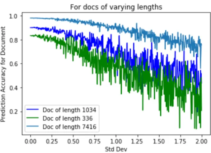
With respect to assuming the noise as a 0-mean Gaussian distribution, the Figures 2.10 and 2.11 show the prediction performance of the model with increasing standard deviation. This noise is added to the embedded test sequence and passed to the initially trained noise free model to predict the probability of the required document. Three ranges are considered here - Documents under 1000 words, between 1000 and 2000 words and over 2000 words.

(25)

(26)

3. TOPIC CLASSIFIER

In the previous chapter, I presented a method to create a doc2vec model. The output of doc2vec may not be entirely satisfactory to a user because it may contain irrelevant contents that are prob-ably “close" to the search query may show up in the results. In order to add a layer of relevance, I use a topic classifier. The challenge that may not be solved is that the term relevance is human centered and highly idiosyncratic. When a user inputs a search query and obtain a relevant “topic" for his search query, he probably was happy with the mixed bag of results the doc2vec model. There might also be a case when a user did not want the relevant topic suggested by my model. If that is the case, then the search query by itself could need revision.

3.2 Related Work

This is one of the most experimented idea in NLP. Topic Classification has been approached in a number of methods. Shallow learning methods including distributed representation were heavily employed because they could efficiently construct high-quality word embeddings and because they could be used for semantic compositionality [4] [18]. Soon, with some drawbacks with word-level embeddings, researchers delved into two sides. The first being character level embeddings and the second completely involving deep neural networks. Zhang,et alused a character-based represen-tation of text as input for a convolutional neural network [19]. The approach’s hope was that if a CNN could learn to interpret the key data, all the labor-intensive work needed to clean and com-pose text could be resolved. Kim,et alwas one of the first to bridge the gap between word vector embeddings and convolutional neural networks [20]. Sentences were converted to embedding vec-tors and made accessible to the system as a matrix output. Convolutions are performed word-wise throughout the output using kernels of different sizes, such as 2 and 3 terms at a time. In order to condense and summarize the extracted functions, the resulting function maps were then processed using a max pooling layer Zhang,et alperformed a sensitivity analysis into the hyper-parameters

(27)

needed to configure a single layer convolutional neural network for document classification [21]. Their aim was to provide general configurations that can be used for configuring CNNs on new text classification tasks. Recently, Attention based networks have shown to get State-of-the-art results in topic classification tasks. Yang, et al introduced the concept of hierarchical attention (HAN) based network that employs sentence level and word level attention [22].

3.2.1 Attention Network

Attention Model, first introduced for Machine Translation [23] has now become a predominant concept in neural network literature. The intuition behind attention can be best explained using human biological systems. For example, our visual processing system tends to focus selectively on parts of the image,while ignoring other irrelevant information in a manner that can assist in per-ception. Let us consider a technical approach to understanding Attention Mechanism. Attention is essentially a map, often with softmax function the inputs of dense layer.Until Attention Mecha-nism, translating depended on reading a full sentence and compressing all data into a fixed-length vector. As you can imagine, a sentence of hundreds of words defined by several words would surely lead to knowledge loss, insufficient comprehension, etc. Be that as it may, Attention partly fixes this issue. It helps the machine translator to display all the information contained in the orig-inal sentence, then produce the correct word according to the actual term on which it operates and the context. It can even zoom in or out (focus on local or global features) for translators.

Probabilistic Language Model’s main crux is to attribute a probability to a Markov Assumption for a sentence. RNN (sequence to sequence (seq2seq)) was naturally applied to model the condi-tional likelihood of words because of the complexity of sentences consisting of different numbers of words. The seq2seq models is normally composed of an encoder-decoder architecture, where the encoder processes the input sequence and encodes/compresses/summarizes the information into a context vector (also called as the “thought vector") of a fixed length. This representation is expected to be a good summary of the entire input sequence. The decoder is then initialized with this context vector, using which it starts generating the transformed output. A critical and

(28)

apparent disadvantage of this fixed-length context vector design is the incapability of the system to remember longer sequences. Often is has forgotten the earlier parts of the sequence once it has processed the entire the sequence. The attention mechanism was born to resolve this problem. The central idea behind Attention is not to throw away those intermediate encoder states but to utilize all the states in order to construct the context vectors required by the decoder to generate the output sequence. In brief, attention in deep learning can be loosely interpreted as a vector of meaning weights: to predict or infer an item, such as a pixel in a picture or a term in a sentence, we calculate how strongly it is associated with (or “attends to" as one may have read in many papers) other elements using the attention function. It then takes the sum of their values weighted by the attention vector as the approximation of the target.

3.2.2 Hierarchical Attention Network

When we think of the textual information nesting structure: character ∈ word∈ sentence ∈

document, a hierarchical emphasis can be built either from top-down (word-level to character-level) or from bottom-up (i.e., word-level to sentence-character-level) to classify hints or to collect important information both globally and locally. Two BiGRUs are used to produce semantic representation at word-level and sentence-level, respectively. To order to obtain a word-level and sentence-level encoding, a pair of hierarchical attention layers are then applied:

h(_it) =BiGRU(v_i(t)) (3.1) vi = X t sof tmax(uT_wh(_it))·h(_it) (3.2) hi =BiGRU(vi) (3.3) c=X t sof tmax(uT_shi)·hi (3.4)

Here,h(_it)andhistand for hidden representation for words and sentences.uTwanduware word-level and sentence-level pattern vectors to be learned during training.The final sentence-level

(29)

represen-tationcis then fed into a logistic regression layer to predict the category.

Figure 3.1: Hierarchical Attention Network [22]

We use this mechanism for document classification and predicting the class labels of documents in the dataset. The dataset used for testing this network is the DBpedia ontology classification dataset.

(30)

3.3 Designs for the Topic Classifier and Integrated Model 3.3.1 Experiment 1

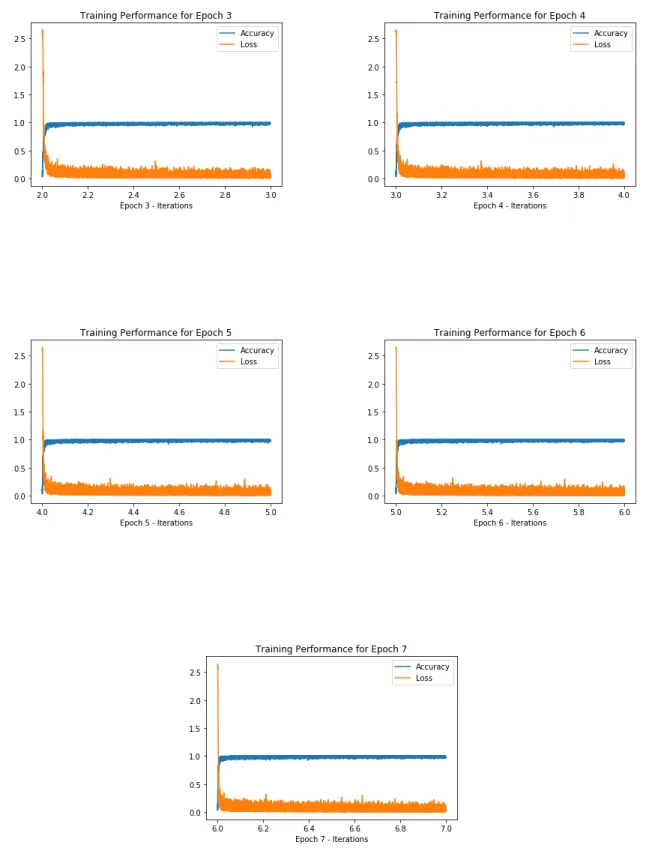
We limit the number of words per sentence to 35and the number of sentences per document to30. A look up dictionary is created in order to encode words to numbers and we obtain a vector for each sentence and a matrix for the whole document. The model was coded to train for 10 epochs with early stopping when the loss was minimized. The training had 4375 iterations for every epoch. The batch size was set to 128. The learning rate was set to 0.1. The model converged to a training accuracy of0.9859with loss as0.0488. Figure 3.3 shows the model performance for each epoch. A closer look at the iterations in an epoch is shown in Figure 3.4. The model at the end of each epoch was saved and on predicting the class labels from the testing data, we get the testing accuracy as0.9864. The confidence interval for this model is the 70000 articles from the DBpedia set. The confusion matrix generated for this test dataset is displayed in Figure 3.2. 3.3.2 Experiment 2

In order to understand this topic classifier better, the embedding dimension was varied and the model was retrained in the same format. From the plots in Figures 3.5 - 3.8, we see that the model accuracy improves with increase in embedding dimension.

3.3.3 Experiment 3

This research focuses on combining the above mentioned applications where we explore a new method of obtaining relevant documents/texts. We analyze the input text using a Hierarchical Attention Network in order to obtain a broad category for the input text. This text, along with the newly learned topic of the text helps to obtain similar documents that are now much more relevant than spatially clustered ones. This model was run through 3 very popular datasets used in text classification.

• The AG News Dataset - The AG News collection comprises of news articles from the web-based database of news articles belonging to the four main groups (World, Business Sports,

(31)

Science / Technology). The dataset contains 30,000 training examples for each class 1,900 examples for each class for testing.

• The DBpedia Ontonlogy Dataset - The DBpedia ontology dataset contains 560,000 training samples and 70,000 testing samples for each of 14 nonoverlapping classes from DBpedia.

• Newsgroups Dataset - The 20 newsgroups dataset comprises around 18000 newsgroups posts on 20 topics split in two subsets: one for training (or development) and the other one for testing (or for performance evaluation).

For each of the cases, we trained a paragraph vector model and a topic classifier model. The results are as shown in Table 3.1 for a random test sample that generated 10 similar documents. In order to justify how the topic classifier works, we use explainable AI techniques(presented in Chapter 3) to justify why our topic classifier picked the right topic.

3.3.4 Experiment 4

In this experiment,we focus on an ensemble learning based approach to topic classifier. Ensem-ble learning is a broad topic and is only confined by one’s own imagination. For this experiment, I have used the 20 Newsgroups dataset.

The hypothesis of ensemble averaging relies on two properties of artificial neural networks - In any network, the bias can be reduced at the cost of increased variance and In a group of networks, the variance can be reduced at no cost to bias.

3.3.4.1 Model Averaging

Every part of the ensemble contributes an equal amount to the final prediction in Model Av-erage. A weighted ensemble is an extension of this average ensemble where each member’s con-tribution is weighted by the model’s performance. The weights of the model are small positive values and sum up to one, allowing the weights to determine the level of confidence or expected performance from each model. Uniform weight values (e.g. _k1 wherekis the number of ensemble

(32)

members) implies the weighted ensemble functions as a simple average ensemble. There is no standard for calculating these weights.

3.3.4.2 Using Shallow Learning Techniques

The three most common approaches for combining multiple models ’ predictions are:

• Bagging - Building multiple models from different sub-sets of the training dataset.

• Boosting - Building multiple models sequentially, where each member learns to fix the pre-diction errors of a prior model in the chain.

• Voting - For combining predictions several models (typically of different types) and basic statistics are used

Bagging works best with high variance algorithms. A common example is decision trees, usu-ally constructed without pruning. In this example, we will explore a Bagged Decision Tree with 100 estimators. A 10 fold cross validation is employed. Random forest is an example of bagged decision trees. Learning information are replicated for substitution, but the trees are constructed in a way that reduces the association between individual classifiers. In general, instead of greedily selecting the best split point in tree building, only a random subset of features are regarded for each split.

AdaBoost may have been the first effective boosting ensemble. algorithm. This operates by weigh-ing cases in the dataset by orderweigh-ing the classification complexity, allowweigh-ing the algorithm to give more or less attention to them as subsequent models are created. One of the most advanced en-semble techniques is stochastic gradient boosting (also called gradient boosting machines). It is a methodology that proves to be perhaps one of the best available techniques to improve perfor-mance by ensembles.

(33)

It essentially creates two or more different models from your testing dataset first. At that stage, a Voting Classifier is utilized to wrap the models and aggregate the sub-model predictions if asked to predict new data.

3.4 Performance Evaluation 3.4.1 Results for Experiment 1

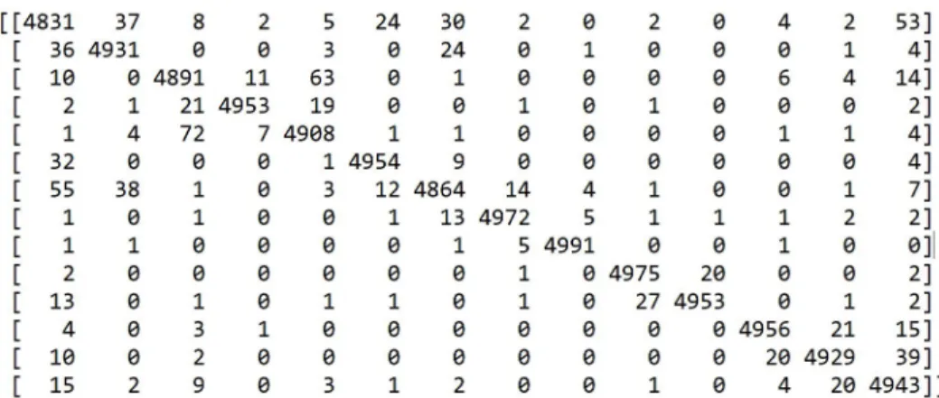
The confusion matrix generated for the test cases in the DBpedia dataset are shown below. The

Figure 3.2: Confusion Matrix generated for the test dataset

(34)

(35)

Figure 3.4: A closer look at the model performance in epoch 7

3.4.2 Results for Experiment 2

(36)

Figure 3.6: Embedding Dimension 100, Number of features = 200,000

Figure 3.7: Embedding Dimension 200, Number of features = 200,000

(37)

The trend for performance plot is shown as a comparison in the Figure 3.9. We see a clear increase in the prediction performance as we increase the embedding dimension.

Figure 3.9: Comparison of the performance of the embedding dimension variants

From the table below, we see a significant improvement in the prediction of the article search tool when it employs the topic classifier.

(38)

AG News DBpedia Newsgroups Cosine Similarity score Cosine Similarity score with topic classifier Cosine Similarity score Cosine Similarity score with topic classifier Cosine Similarity score Cosine Similarity score with topic classifier 0.4918 0.6118 0.7214 0.8516 0.6017 0.7452 0.4903 0.5877 0.7156 0.7910 0.6013 0.6988 0.4902 0.5797 0.7102 0.7843 0.5982 0.6872 0.4856 0.5634 0.6817 0.7612 0.5881 0.6776 0.4833 0.5612 0.6624 0.7500 0.5582 0.6211 0.4611 0.5499 0.6391 0.6921 0.5521 0.6019 0.4207 0.5435 0.5801 0.6345 0.5517 0.6008 0.4002 0.5388 0.5789 0.6257 0.5499 0.5912 0.3844 0.5369 0.5721 0.5912 0.5112 0.5910 0.3844 0.5364 0.5721 0.5816 0.4998 0.5800

Table 3.1: Cosine similarity score for the top 10 generated documents with and without the topic classifier

Plotting this table, we see a comparison for the 3 datasets as shown in Figure 3.10.

Figure 3.10: Comparison of Prediction Accuracy of the Integrated model and Doc2vec model for the 3 datasets

(39)

3.4.3.1 Query Generation

In order to generate search queries for evaluation, I removed 2-3 random words from a sentence in a document and replace them with their synonyms. I then observe if my model can capture the same document.

For example, if the document “Sentence with all alphabets" has a sentence The quick brown fox jumped over the lazy dog, my generated query will look likeThe rapid fox over lazy dog

3.4.3.2 Evaluation of the Integrated model

While so far, we have dealt with this problem as an unsupervised task, we can make it a super-vised task in the following manner

• For each of the document in the database, I created an input-label pair of Document and its title.

• Instead of splitting the document into train and test, I will train it on the whole dataset with the words already present in the document and test on a subset of the dataset using the search query for each.

• For each of the document, I will pick a sentence at random and create a test query as men-tioned above.

• Predict the set of documents.

• If my test document is present in the output set of documents with a cosine similarity score greater than a threshold value, I will count that as a correct prediction.

The above procedure will help to evaluate my approach in a supervised setting. In order to show why using my integrated model is better, the same approach is followed. The following are the evaluation results.

(40)

Figure 3.11: Comparison of Prediction Accuracy of the Model with respect to Threshold for pre-diction

The figure 3.11 shows a comparison of the prediction accuracy for arbitrarily generated test queries for 140,000 documents in the DBpedia dataset. The integrated model fares better than the doc2vec. We see that the documents can be predicted accurately in comparison to just the doc2vec model. In this plot, I varied the threshold for considering as a prediction. This means that when the cosine similarity for the document is less than the threshold, I label it as an incorrect predic-tion. The doc2vec model’s performance drops sharply over threshold values greater than 0.5. This indicates that the doc2vec model returns documents with distance roughly around this threshold value. This is not observed in the integrated model because the model predicts documents almost surely for a threshold of 0.79 and reduces after 0.93 threshold. This value will never be equal to 1 because the my query string is not the same as the strings in my document.

(41)

3.4.3.3 Discussion

In the analysis above, I mentioned that I generate the queries for each document and observe the prediction based on a threshold. In order to validate my approach, let us look at how the true labels are created for this supervised task. Since my end goal is to predict the document, I will label all documents as class 1. At the prediction time, based on the observed value and threshold, I will assign the predicted labels to each of the documents in my test cases. Now, in a general scenario, the ground truth is given to us already and it does not depend on the task/method that follows. However, in this setting, I try to induce a supervised task setting and hence my ground truth for all documents is class 1.

3.4.3.4 Why my topic classifier helps in my integrated model

Topic Classifier adds relevance to my search query. Doc2vec model alone outputs documents that are generic and uses a distance metric. Now the question automatically becomes what is rel-evance? The definition for relevance in Wikipedia is Relevance is the concept of one topic being connected to another topic in a way that makes it useful to consider the second topic when con-sidering the first. Relevance has proven to be a critical yet difficult term in formal analysis. Any problem requires the prior definition of the underlying principles from which a solution can be constructed. It is enigmatic, because in ordinary coherent structures, the sense of relevance tends to be problematic and incomprehensible.

Let us try to visualize this. Consider an event where you ask a friend to fetch an object from your house. Now let us also assume that this friend has never been inside your house. When you simply give this person the task and not provide any other information, he will go through the entire house till he finds it. Now, if we provide this person an extra piece of information that this object is near the study table, the person’s search space is lesser and he is likely to find the object faster. This is exactly what I aim to do in my integrated model.

(42)

3.4.4.1 Model Averaging - Using only fully connected layers

We extract the features from the newsgroups dataset. The neural network used has 1 hidden layer with 100 nodes, ReLU activated and the output layer has 20 nodes. The model is fit for 25 epochs. An ensemble is created with 10 members. We have the following result, comparing the performance of the classifier with and without the ensemble.

Figure 3.12: Single model versus Ensembles

3.4.4.2 Model Averaging - Using HAN

While this is the state of the art method for topic classifiers, there was not much increase in prediction accuracy in using the HAN with model averaging technique. The method remained same as what was in the previous case. We have the following result:

(43)

Figure 3.13: Single model versus Ensembles

3.4.4.3 Shallow Learning approach

We have the following results for the shallow learning methods on the 20 Newsgroups dataset.

Method Num Trees Mean Test Accuracy Training Time (approx)

Adaboost 200 0.912 4 hours

Bagged Decision Trees 100 0.8876 7 hours

Random Forest 200 0.8908 4 hours

Gradient Boosting 100 0.7126 2 hours

Voting Ensemble NA 0.8911 4 hours

Table 3.2: Mean Test performance of commonly used ensemble techniques

3.5 Applications

While I have shown a few examples where this topic classifier can be applied, there are various other areas where the model can be applied. I introduce the same model with an additional Batch Normalization layer for the sentence encoder and present 3 more examples to show the effect of Embedding variants of the HAN model. For this particular example alone, I will show the comparison of the techniques using XAI in the next section.

(44)

3.5.1 Medical Text Classifier (MTC)

In this publicly available dataset, we have around 10,000 abstracts for training, 1400 for val-idation and 2800 for testing. It is important to understand that these are medical datasets and it is highly likely that the labels can overlap to a large extent. Since we have 5 classes, the baseline prediction accuracy is 0.20, while our variants perform far better. The table below shows the model performance values. The 5 classes in this dataset are Neoplastic Diseases, Digestive System Dis-eases, Nervous System DisDis-eases, Cardiovascular Diseases and General Pathological Conditions. The results below show the model performance for the 4 different embedding variants.

Embedding Size Train_acc Train_loss Test_acc Test_loss Epochs

50 0.7012 0.7092 0.6014 0.9263 11

100 0.7085 0.7129 0.5959 0.9903 9

200 0.7197 0.6909 0.5872 1.0282 8

300 0.7282 0.6712 0.6049 1.0001 7

Table 3.3: MTC - Comparison of the model performance with embedding size

3.5.2 Web of Science Dataset

Web of Science (previously known as Web of Knowledge) [24] is a website which provides subscription-based access to multiple databases that provide comprehensive citation data for many different academic disciplines. It has 7 major classes namely Computer Science, Electrical Engi-neering, Psychology, Mechanical EngiEngi-neering, Civil EngiEngi-neering, Medical Science and Biochem-istry. The results below show the model performance for the 4 different embedding variants. From this dataset, we have around 28,000 abstracts for training, 10,000 for validation and 10,000 for testing.

(45)

50 0.8960 0.2975 0.8508 0.4825 19

100 0.8885 0.3165 0.8525 0.4751 16

200 0.9223 0.2391 0.8947 0.3118 8

300 0.9318 0.2043 0.9018 0.2918 7

Table 3.4: WoS - Comparison of the model performance with embedding size

3.5.3 Kaggle Cancer Gene Mutation Dataset

Memorial Sloan Kettering Cancer Center (MSKCC) launched a kaggle competition to classify genetic mutations based on clinical evidence (text). There are nine different classes a genetic mu-tation can be classified on (Labeled from 1-9). The results below show the model performance for the 4 different embedding variants.

50 0.4219 1.2975 0.3508 1.7825 35

100 0.4247 1.4876 0.4019 1.7000 26

200 0.4621 1.2284 0.4647 1.6118 16

300 0.4718 1.2043 0.4718 1.3918 16

Table 3.5: CGM - Comparison of the model performance with embedding size

From the above results, if we plot the table values (Figure 3.14), we see that the increase in em-bedding dimension once again shows an increase trend in performance of the HAN model.

(46)

(47)

4. EXPLAINABLE AI TECHNIQUES

The main drawback of black-box models, as the name suggests, is its inability to explain the underlying computation. While they can be very powerful for predictive analysis, it is important to know why they work. We blindly trust the recommendations of friends of Facebook, movie recommendations on Netflix and Amazon. However, we do not have the same level of trust when it comes to medical applications or actions involving life and property. This challenge is overcome by using Explainable AI.

4.2 Related Works

We divide the strategies into 3 categories

-• based on complexity of interpretability

• based on grasp of interpretability

• based on level of dependency from the learning model in that problem. 4.2.1 Complexity related strategy

A machine learning model’s sophistication is directly linked to its interpretability. Generally speaking, the more complicated the model, the harder it is to understand and justify. Rule Lists and Decision trees are the most common intrinsic strategies that support the idea of making the model itself interpretable [25] [26]. However, as mentioned above, this level of interpretability trades off with the accuracy of the model. While some specific tasks in the industry involve a small number of data point (where experiments to generate data points are expensive), such model specific methods can be employed. In deep learning sense, there have been some authors who have used the attention mechanism it self to interpret the model behavior [27] [28], many have given counter examples to show merely attention is not a fail safe method for model interpretability [29] [30].

(48)

4.2.2 Interpretability via Scoop

This strategy supports two methods - comprehension of the whole model action (Global In-terpretability) or a particular instance (Local InIn-terpretability). Global interpretability enables the interpretation of a model’s whole meaning and supports the whole theory leading to all the various possible consequences. This can be attributed to how the features affect class variables. While a significant number of methods are used in literature to allow global interpretability [31][32][?], it is arguably difficult to achieve global model interpretability in reality, especially for models that exceed a limited set of parameters. Local interpretability can be more readily applicable to humans who focus attention on only part of the system to comprehend the whole of it. So, the aim here is to generate an individual explanation, generally, to legitimize why the model made a particular decision for an instance. While there are many locally interpretable models [34] [35], we have 2 major contributions in this area - LIME [36] and SHAP [37].

4.2.2.1 LIME

The local explanation method LIME interprets an individual prediction by learning an inter-pretable model locally. The intuition behind LIME is that it samples instances both in the vicinity and far away from the interpretable representation of the original input. Then LIME takes the inter-pretable representation of these sample points, determines their predictions and builds a weighted linear model by minimizing the loss and complexity. The samples weighting is based on their distances from the original point. The points weights decrease as the points get farther away. The explanation is locally faithful, which means it represents the model prediction of vicinity instances. Let us look at this intuition mathematically.

Let f denote the complex model being explained. f(x) is the probability that an instancex be-longs to the certain class. Let g be defined as explanation model g ∈ G, where Gis a class of

(49)

interpretable models, such as linear models and decision trees. If we assume a linear model,

g(z0) = wg ·z0 (4.1)

Also, x ∈ RN _where _N _{is the number of features in the original input. A mapping function is} defined to convert the binary pattern of missing features represented byx0 to its original feature value

x=hx(x0) (4.2)

LIME draws samples aroundx0 uniformly at random. Given a perturbed samplez0, LIME can re-cover the sample to its original inputzand obtainf(z), which is used as a label for the explanation model. As we know, LIME generates the explanationξby minimizing the loss

ξ(x) = argmin g∈G

L(f, g, πx) + Ω(g) (4.3)

The first term measures how unfaithfulgis in approximatingf. The second term is the complexity of the model. The proximity measure betweenxandzis denoted as an exponential kernelπx. The lossLis computed by weighted square loss whereπx(z). is an exponential kernel defined on some distance function with width.

L(f, g, πx) = X z,z0_∈Z πx(z) f(hx(z0)−g(z0) 2 (4.4)

To solve the above equations and to obtain the explanation, LIME approximatesΩ(g)by selecting K features with Lasso and then learning the weights via least squares.

Now, how does LIME go over this procedure?

• Enablen times for each prediction to justify. The permutations are done by randomly ex-pelling terms from the initial example when the product of text projections is to be explained

(50)

Based on whether or not the model uses word location, words that appear several times will be removed whether one-by-one or entirely.

• Let the black box model predict the result of all permuted cases.

• Measure the distance to the original from all permutations.

• Transfer the distance to a ranking of similarities based on score. As permutations are gen-erated on the basis of inputs separately, comparisons are measured in various ways. The cosine similarity measure is used for text data which is the norm in text analysis (the angle difference between the two attribute vectors is effectively measured).

• Choose m best features from the permuted data to reflect the complex model’s outcome. Choice of features is a full sub-field of modeling in itself and there’s no silver bullet for LIME. Instead, it implements a variety of solutions to the choice of options that an user can choose from.

• Fit a simple model to the permuted data, explaining the black box model output with the m features of the permuted data weighted by its similarity to the original instance.

• Extract the weights of the function from the simple model and use them to illustrate the local behavior of the black box model.

The reliability of the model or the metric of consistency (how well the interpretable model ap-proximates the predictions of the black box) gives us a great perspective into how accurate the interpretable model is to explain the predictions of the black box in the information instance of in-terest. The examples of regional surrogate models may use features other than the original model. This will be a huge advantage over other approaches when it is not possible to interpret the original features. A text classifier can rely on conceptual word embedding as attributes, but the interpreta-tion may be dependent on a sentence’s presence or absence of letters. The authors followed up on LIME by introducing another paper that fortified results from LIME [9]. It had a limitation that al-though we can use simple function to interpret complexity locally, it can only explain the particular

(51)

instance. It means that it may not able to fit for unseen instance. Anchors, the new strategy, uses “local region” to learn how to explain the model. The “local region” refer to a better construction of generated data set for explanation.

4.2.2.2 SHAP

Shapley value is a concept of solution in game theory. TThe aim is to use game theory to view the goal model. All features are "contributor" and attempting to predict the "game" task and the "reward" is the actual prediction minus the explanation model result. Shapley value is the average contribution of features which are predicting in different situation. In other word, it is not talking about the difference when the particular feature missed. The authors of SHAP prove in their NIPS paper that the values of Shapley are the only guarantee of reliability and continuity and that LIME is in essence a subclass of SHAP which lacks the same properties.

In order to understand SHAP values, let us look at a small example. Consider a development team. Our aim is to create a deep learning framework that allows 100 line of codes to be completed while we have 3 data scientists (L, M, N).

V(x) Lines of code L 10 M 30 N 5 L,M 50 L,N 40 M,N 35 L,M,N 100

(52)

We calculate the marginal contribution through all permutations of players.

Order L Contribution M Contribution N Contribution

L,M,N V(L) = 10 V(L,M) - V(L) = 50-10 = 40 V(L,M,N) - V(L,M) = 100-50 = 50 L,N,M V(L) = 10 V(L,M,N) - V(L,N) = 100-40 = 60 V(L,N) - V(L) = 40-10 = 30 M,L,N V(L,M) - V(M) = 50-30 = 20 V(M) = 30 V(L,M,N) - V(L,M) = 100-50 = 50 M,N,L V(L,M,N) - V(M,N) = 100-35 = 65 V(M) = 30 V(M,N) - V(M) = 35-30 = 5 N,L,M V(L,N) - V(L) = 40-10 = 30 V(L,M,N) - V(L,N) = 100-40 = 60 V(N) = 5 N,M,L V(L,M,N) - V(M,N) = 100-35 = 65 V(M,N) - V(M) = 35-30 = 5 V(N) = 5

Table 4.2: Marginal Contribution by different orders

The shapley value is given by:

φi(v) = 1 |N|! X R h vP_iR∪ {i}−vP_iRi (4.5) where

φis the Shapley value, N is the number of players, PR

i is the set of player with order,

vP_iRis the contribution of set of player with that order,

(53)

So, from Table 4.2 and the above Equation, we can compute the Shapley values for each of the players as

Player Shapley Calculation Shapley Value L (1/3! )(10+10+20+65+30+65) 33.33

M (1/3! )(40+60+30+30+60+5) 37.5

N (1/3! )(50+30+50+5+5+5) 24.17

Table 4.3: Shapley value for each player

These values makes sense because player N does least work individually, and hence has a much lower Shapley value compared to L and M. In our examples, it is difficult to show by hand cal-culations, the effect of each feature permuted with the rest. As a result, we can only interpret the importance of each feature per class label from the summary plot.

While we have seen a great amount of consistency in the reason for class prediction over all the cases, there are obviously some differences. Trivially, this is because the methods used are completely different. SHAP, as the title of the paper says is a Unified approach to model inter-pretability. It combines multiple methods and produces an optimized pipeline. Nevertheless, all the 3 models have issues related to efficiency. SHAP, especially, has proven to be extremely useful in interpreting tabular data. The authors have introduced KernelSHAP and DeepSHAP. Before we go over the mathematics behind these methods, let us see the 3 useful properties of shapley values.

• Property 1 -Local Accuracy

f(x) =g(x0) = φ0+

M

X

i=1

φix0i (4.6)

The explanation modelg(x0)matches the original modelf(x)whenx=hx(x0), whereφ0 =

(54)

• Property 2 -Missingness

x0_i = 0 =⇒ φi = 0 (4.7)

Missingness constrains features wherex0_i = 0to have no attributed impact.

• Property 3 -ConsistencyLetfx(z0) = f(hx(z0)) andz0\xdenote setting zi0 = 0. For any two modelsf andf0, if

f_x0(z0)−f_x0(z0\i)≥fx(z0)−fx(z0\i) ∀z0 ∈ {0,1}M (4.8)

then,

φi(f0, x)≥φi(f, x) (4.9)

This leads us back to the Equation 4.5, where we can rewrite the same as

φi(f, x) = X z0_⊆x0 |z0|!(M − |z0| −1)! M! fx(z0)−fx(z0\i) (4.10)

where|z0|is the number of non-zero entries inz0, andz0 ⊆ x0 represents allz0 vectors where the non-zero entries are a subset of the non-zero entries inx0.

These shapley values, as mentioned in the above equations and example, are the conditional expectation function of the original model, i.e the solution to Equation 4.10. Here, fx(z0) = f(hx(z0)) = E[f(z)|zS], where S is the set of non-zero indices in z0. The authors proposed DeepSHAP as a way to combine Shapley values and the DeepLIFT technique to interpret deep learning models. The summation-to-delta property in DeepLIFT states that

n

X

i=1

C∆xi∆o = ∆o (4.11)

(55)

input. Here, if we chooseφi =C∆xi∆o andφ0 asf(r), we get our original idea of additive feature

attribution. From the explanation of conditional distribution, if we assume model linearity and feature independence, we get

f(hx(z0)) =E[f(z)|zS] (4.12) =EzS¯|zS f(z) S /¯∈S (4.13) ≈Ez_S¯ f(z) (4.14) ≈f zS, E[z_S¯] (4.15)

If we interpret the reference value in summation-to-delta equation and the above conditional distribution approximation, then DeepLIFT approximates SHAP values assuming that the input features are independent of one another and the deep model is linear. Since DeepLIFT is an ad-ditive feature attribution method that has local accuracy and missingness property, Shapley value bridges the remaining consistency property in helping us arrive at DeepSHAP.

DeepLIFT’s multiplication rule is given by

m∆x∆t =

C∆x∆t

∆x (4.16)

In other words, it is the ratio of contribution of difference-from-reference to input neuron ∆xto difference-from-reference to target neuron∆tto the difference-from-reference to input neuron∆x. Note the close analogy to the idea of partial derivatives where _∂x∂t is the infinitesimal change in t caused by an infinitesimal change in x, divided by the infinitesimal change in x. The multiplier is similar in spirit to a partial derivative, but over finite differences instead of infinitesimal ones. Writing this multiplier in terms of shapley coefficients for backpropagation, we get the linear approximation for shapley values in terms of DeepLIFT.

(56)

Figure 4.1: DeepSHAP interpretation [37] mxjf3 = φi f3, x xj−Exj (4.17) ∀j∈{1,2} myifj = φi fj, y yi−Eyi (4.18) myif3 = 2 X j=1 myifjmxjf3 (chain rule) (4.19)

This chain rule is given by

m∆xi∆t=

X

j

m∆xi∆yjm∆yj∆t (4.20)

wherex1, x2, x3, ...are input neurons,y1, y2, y3, ..are neurons in a hidden layer and target ist.

Linearly approximating Equation 4.17, we get the shapley value for the feature as

φi(f3, y)≈myif3 yi−E yi (4.21)

(57)

4.2.2.3 ELI5

We also have a python package ELI5 - Explain Like I’m 5 [38]! ELI5 provides both global model interpretation and local model interpretation. The global model interpretation can be con-sidered simply as a feature importance. It not only support decision tree algorithm such as Random Forest and XGBoost but also all scikit learn estimators. ELI5 author introduces it as Permutation Importance for global interpretation. To calculate the score, feature (a word) will be replaced by other word (noise) and predicting it. The idea is that feature importance can be deduced by getting how much score decrease when a particular word is not provided.

4.2.3 Model related methods

Another effective way to define model interpretability techniques is that if they are agnostic methods, meaning they can be extended to any form of ML algorithms, or model-specific tech-niques, meaning techniques that are only applicable to a particular algorithm category or class. The downside to intrinsic method practice is that when we need a particular type of analysis, we are limited to the models that provide it in terms of selection, possibly at the cost of using a more accurate and representative model. Model-agnostic representations are normally post-hoc, commonly used to explain neural networks, and could be local or global structures that can be interpreted. There are four main categories of agnostic simulation techniques

-• Visualization - Visualization techniques are applied primarily to supervised models of learn-ing. Popular visualization techniques include: Surrogate models, Partial Dependence Plot (PDP) [39] and Individual Conditional Expectation (ICE) [40].

– These are models that are simple to explain a complex model. In general, it is an interpretable model (like a regression model or decision tree) that is learned to approach the latter on the assumptions of the original black-box model. There are, however, almost no empirical assurances that the more complex version is strongly reflective of the basic surrogate model. The LIME methodology described above is a recommended method for constructing regional surrogate models around [36] single observations.

(58)

– PDP - This is a visual representation that helps to illustrate the partial average associa-tion of one or more input parameters and a black-box model’s predicassocia-tions.

– ICE - ICE plots extend PDP. While PD plots provide a fuzzy view of the workings of a system, ICE plots show relationships and individual differences by breaking down the PDP performance.

• This can be important inner representations when learning algorithms change cells in the hidden surface. Therefore, the function of extracting explanations from the network is to re-move the knowledge acquired through learning and encoded as an internal representation[41] in a comprehensible manner.

• Influence methods - This method of techniques measures the value and importance of a function by adjusting the output or internal components and observing how the changes affect the performance of the design.

– Sensitivity Analysis - Sensitivity refers to how the source and/or weight interference of an ANN output is affected. It is used to verify that model behavior and outputs remain stable when intentionally disrupting data or simulating other changes in data. Visual-izing the results of sensitivity analysis is regarded an agnostic interpretation strategy, as the view of stability models as data shift increases confidence in the performance of machine learning [42].

– Layer-wise Relevance Propagation - This strategy consolidates the prediction function backwards, originating from the output layer of the network and backpropagating to the input layer. The main property of this phase of restructuring is called preservation of interest. This approach discusses predictions relevant to the state of peak uncertainty [43] as opposed to sensitivity analysis.

– Feature Importance - Variable importance assesses each input variable’s contribution (feature) to a complicated ML model’s predictions. The change in the prediction error of the system is determined after the feature has been permutated to measure the value

(59)

of a function. It increases the model error by allowing the values of important features. The model ignores the values of unimportant features when permuting and thus holds [44] unchanged model error.

• Example based explanation - Example based explanation techniques select particular in-stances of the dataset to explain the behavior of machine learning models. Example-based explanations are mostly model agnostic because they make any ML model more interpretable [45].

4.3 Designs

4.3.1 Experiment 1

Given a random test input, I generate explanations for the topic classifier model using the XAI techniques.

4.3.2 Experiment 2

In Experiment 2 in Section 2, we varied embedding dimensions for the HAN model. Here, I will generate explanations for each embedding variant to compare and show the improvement in the prediction performance.

4.3.3 Experiment 3

This experiment focuses on the idea of model tuning using XAI techniques. For this, I will generate explanations for the topic classifier as it trains.

4.3.4 Experiment 4

As mentioned in Section 3.3.2, the new HAN with a batch normalized layer has been compared with the embedding dimension variant along with the XAI techniques.

(60)

4.4 Performance Evaluation 4.4.1 Result for Experiment 1

Consider a random test input:

Input Text: Share prices for the British drugmaker Indivior plunged today on the London Stock Exchange. The drop came on news that the U.S. Justice Department indicted the company on fraud and conspiracy charges. Indivior makes the drug Suboxone, widely used to treat people suffering from opioid addiction. Federal prosecutors now claim the company falsely marketed Suboxone as safer and less prone to abuse than cheaper generic drugs. North Country Public Radio’s Brian Mann reports.

Thepredicted classfrom the hierarchical attention network is : Company. The attention weights for the words are shown below, sentence-wise.

(61)

Figure 4.2: Attention weights for words in every sentence

(62)

Next we look at the output from LIME, Eli5 and Shap.

(63)

(64)

Figure 4.6: SHAP summary plot - Class labels correspond to 0: ’Company’, 1: ’Educational In-stitution’, 2: ’Artist’, 3: ’Athlete’, 4: ’Office Holder’, 5: ’Mean Of Transportation’, 6: ’Building’, 7: ’Natural Place’, 8: ’Village’, 9: ’Animal’, 10: ’Plant’, 11: ’Album’, 12: ’Film’, 13: ’Written Work’

(65)

The table below highlights Which words are missing and which are found in common among the 4 methods discussed above. The color coding is as follows: Yellow - 2 similar words ; Light Green - 3 similar words ; Dark Green - All models have the words

Similar words and Dissimilar words

Attention Network LIME SHAP Eli5

News Company Opioid Share

Department Stock Prosecutors Price

Company Cheaper Safer Stock

Justice Opioid Plunged Exchange

Indicted Generic Indicted Company

Came Exchange Falsely Charges

Make Cheaper Makes

British Share Opioid

Drug Prone Fraud

Plunged Fraud Federal

Conspiracy Conspiracy Cheaper

Fraud Prices Generic

Today Addiction Marketed

People Treat London Charges Price Abuse Drugmaker Generic Charges Suffering Treat Drop Suboxone Drugs Widely Share Stock Used Exchange Suffering Opioid Addiction