Calhoun: The NPS Institutional Archive
Theses and Dissertations Thesis Collection
2009-09
Characteristics of the binary decision diagrams of
Boolean Bent Functions
Schafer, Neil Brendan.
Monterey, California: Naval Postgraduate School
NAVAL
POSTGRADUATE
SCHOOL
MONTEREY, CALIFORNIA
THESIS
Approved for public release; distribution is unlimited CHARACTERISTICS OF THE BINARY DECISION
DIAGRAMS OF BOOLEAN BENT FUNCTIONS
by
Neil Brendan Schafer September 2009
Thesis Advisor: Jon T. Butler
REPORT DOCUMENTATION PAGE Form Approved OMB No. 0704-0188 Public reporting burden for this collection of information is estimated to average 1 hour per response, including the time for reviewing instruction, searching existing data sources, gathering and maintaining the data needed, and completing and reviewing the collection of information. Send comments regarding this burden estimate or any other aspect of this collection of information, including suggestions for reducing this burden, to Washington headquarters Services, Directorate for Information Operations and Reports, 1215 Jefferson Davis Highway, Suite 1204, Arlington, VA 22202-4302, and to the Office of Management and Budget, Paperwork Reduction Project (0704-0188) Washington DC 20503.
1. AGENCY USE ONLY (Leave blank) 2. REPORT DATE
September 2009 3. REPORT TYPE AND DATES COVEREDMaster’s Thesis
4. TITLE AND SUBTITLE
Characteristics of the Binary Decision Diagrams of Boolean Bent Functions
6. AUTHOR(S) Neil Brendan Schafer
5. FUNDING NUMBERS
7. PERFORMING ORGANIZATION NAME(S) AND ADDRESS(ES)
Naval Postgraduate School Monterey, CA 93943-5000
8. PERFORMING ORGANIZATION REPORT NUMBER
9. SPONSORING /MONITORING AGENCY NAME(S) AND ADDRESS(ES)
N/A
10. SPONSORING/MONITORING AGENCY REPORT NUMBER
11. SUPPLEMENTARY NOTES The views expressed in this thesis are those of the author and do not reflect the official policy
or position of the Department of Defense or the U.S. Government.
12a. DISTRIBUTION / AVAILABILITY STATEMENT
Approved for public release; distribution is unlimited A 12b. DISTRIBUTION CODE
13. ABSTRACT (maximum 200 words)
Boolean bent functions have desirable cryptographic properties in that they have maximum nonlinearity, which hardens a cryptographic function against linear cryptanalysis attacks. Furthermore, bent functions are extremely rare and difficult to find. Consequently, little is known generally about the characteristics of bent functions.
One method of representing Boolean functions is with a reduced ordered binary decision diagram. Binary decision diagrams (BDD) represent functions in a tree structure that can be traversed one variable at a time. Some functions show speed gains when represented in this form, and binary decision diagrams are useful in computer aided design and real-time applications.
This thesis investigates the characteristics of bent functions represented as BDDs, with a focus on their complexity. In order to facilitate this, a computer program was designed capable of converting a function’s truth table into a minimally realized BDD.
Disjoint quadratic functions (DQF), symmetric bent functions, and homogeneous bent functions of 6-variables were analyzed, and the complexities of the minimum binary decision diagrams of each were discovered. Specifically, DQFs were found to have size 2n – 2 for functions of n-variables; symmetric bent functions have size 4n – 8, and all homogeneous bent functions of 6-variables were shown to be P-equivalent.
15. NUMBER OF PAGES
175
14. SUBJECT TERMS
Binary Decision Diagrams, Boolean Bent Functions, Homogeneous Functions, Disjoint Quadratic Functions, Symmetric Bent Functions, P-Equivalence, Minimization, Hardware Complexity, Circuit
Complexity, Graphical Interface, Nonlinearity, Hamming Distance, Cryptography 16. PRICE CODE
17. SECURITY CLASSIFICATION OF REPORT Unclassified 18. SECURITY CLASSIFICATION OF THIS PAGE Unclassified 19. SECURITY CLASSIFICATION OF ABSTRACT Unclassified 20. LIMITATION OF ABSTRACT UU NSN 7540-01-280-5500 Standard Form 298 (Rev. 2-89)
Approved for public release; distribution is unlimited
CHARACTERISTICS OF THE BINARY DECISION DIAGRAMS OF BOOLEAN BENT FUNCTIONS
Neil Brendan Schafer Lieutenant, United States Navy
BSCpE, Virginia Tech, 2004 Submitted in partial fulfillment of the
requirements for the degree of
MASTER OF SCIENCE IN ELECTRICAL ENGINEERING
from the
NAVAL POSTGRADUATE SCHOOL September 2009
Author: Neil Brendan Schafer
Approved by: Jon T. Butler
Thesis Advisor
Pantelimon Stanica Thesis Co-Advisor
Professor Jeffrey B. Knorr
ABSTRACT
Boolean bent functions have desirable cryptographic properties in that they have maximum nonlinearity, which hardens a cryptographic function against linear cryptanalysis attacks. Furthermore, bent functions are extremely rare and difficult to find. Consequently, little is known generally about the characteristics of bent functions.
One method of representing Boolean functions is with a reduced ordered binary decision diagram. Binary decision diagrams (BDD) represent functions in a tree structure that can be traversed one variable at a time. Some functions show speed gains when represented in this form, and binary decision diagrams are useful in computer aided design and real-time applications.
This thesis investigates the characteristics of bent functions represented as BDDs, with a focus on their complexity. In order to facilitate this, a computer program was designed capable of converting a function’s truth table into a minimally realized BDD.
Disjoint quadratic functions (DQF), symmetric bent functions, and homogeneous bent functions of 6-variables were analyzed, and the complexities of the minimum binary decision diagrams of each were discovered. Specifically, DQFs were found to have size 2n – 2 for functions of n-variables; symmetric bent functions have size 4n – 8, and all homogeneous bent functions of 6-variables were shown to be P-equivalent.
TABLE OF CONTENTS
I. INTRODUCTION...1
A. PROBLEM DEFINITION ...1
B. THESIS GOALS ...2
C. THESIS ORGANIZATION...2
II. BOOLEAN FUNCTIONS AND THEIR CRYPTOGRAPHIC PROPERTIES ....3
A. BOOLEAN FUNCTIONS ...3
1. Algebraic Normal Form ...4
2. Algebraic Degree...4 3. Linear Functions ...4 4. Affine Functions ...5 5. Hamming Weight ...5 6. Hamming Distance...5 B. CIPHERS...5 1. Plaintext ...5 2. Cryptographic Key ...6 3. Ciphertext ...6 4. Cipher Example ...6 5. Cryptographic Properties ...7 C. BENT FUNCTIONS ...8 1. Definitions...8 a. Nonlinearity...8 b. Bent Functions...9
2. The Difficulty of Discovering Bent Functions ...9
a. Lower Bound...10
b. Upper Bound ...10
c. Enumerations ...10
3. Known Bent Functions ...11
a. Disjoint Quadratic Functions...11
b. Symmetric Bent Functions ...12
c. Constructing Bent Functions ...15
D. SUMMARY ...15
III. BINARY DECISION DIAGRAMS...17
A. BINARY DECISION DIAGRAM CONSTRUCTION ...17
1. Binary Decision Tree ...17
2. Quasi Reduced Ordered Binary Decision Diagrams ...19
a. The Ordered Property ...19
b. The Quasi Reduced Property...19
3. Reduced Ordered Binary Decision Diagrams ...21
B. BINARY DECISION DIAGRAM COMPLEXITY ...23
1. Maximum Complexity of a Reduced Ordered Binary Decision Diagram ...25
2. Variable Ordering...26
C. BINARY DECISION DIAGRAM APPLICATIONS...29
1. Binary Decision Machines...29
2. Quaternary Decision Diagram Machine...30
D. SUMMARY ...31
IV. BDDVIEWER ...33
A. REDUCTION PROCESS...34
1. A High Level View of the Problem...34
2. Pseudo Code ...38
B. MINIMIZATION...39
1. Johnson-Trotter Adjacent Transposition Algorithm ...39
2. Pseudo-Code for Johnson-Trotter...41
3. Example Permutation...41
4. Truth Table Application of the Input Variable Permutation Algorithm...42
5. Pseudo-Code for Truth Table Manipulation...46
C. SUMMARY ...46
V. DISCOVERIES ...47
A. DISJOINT QUADRATIC FUNCTIONS ...47
B. SYMMETRIC BENT FUNCTIONS...50
C. HOMOGENEOUS BENT FUNCTIONS OF ORDER SIX AND ALGEBRAIC DEGREE THREE ...54
D. AFFINE CLASSES...60
E. SUMMARY ...61
VI. CONCLUSIONS AND FUTURE WORK ...63
A. CONCLUSIONS ...63
B. FUTURE WORK ...64
1. On BDDs and Bent Functions...64
2. BDDViewer...65
APPENDIX A: CODE ...67
A. TEXT-BASED TREE DATA STRUCTURE ...67
B. GRAPHICS-BASED TREE DATA STRUCTURE...73
C. MAIN: OPENGL AND CONSOLE APPLICATION ...82
APPENDIX B: DISJOINT QUADRATIC FUNCTIONS ...95
A. DISJOINT QUADRATIC AFFINE CLASS OF ORDER 2 ...95
B. DISJOINT QUADRATIC AFFINE CLASS OF ORDER 4 ...98
C. PARTIAL DISJOINT AFFINE CLASS OF ORDER 6...107
D. PARTIAL DISJOINT QUADRATIC AFFINE CLASS OF ORDER 8 .128 APPENDIX C: SYMMETRIC BENT FUNCTIONS...135
APPENDIX D: MISCELLANEOUS BDDS...139
A. PARTIAL SELECTION OF HOMOGENEOUS FUNCTIONS ON
8-VARIABLES OF DEGREE 3 (MINIMUMS BDDS) ...139
B. MISCELLANEOUS 8-VARIABLE BENT FUNCTIONS (MINIMUM
BDDS)...147 LIST OF REFERENCES ...151 INITIAL DISTRIBUTION LIST ...153
LIST OF FIGURES
Figure 1. A simple cipher using a 12-bit key. ...6
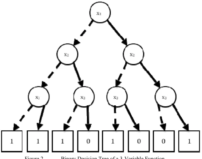
Figure 2. Binary Decision Tree of a 3-Variable Function...18
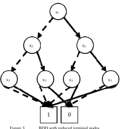
Figure 3. BDD with reduced terminal nodes...20
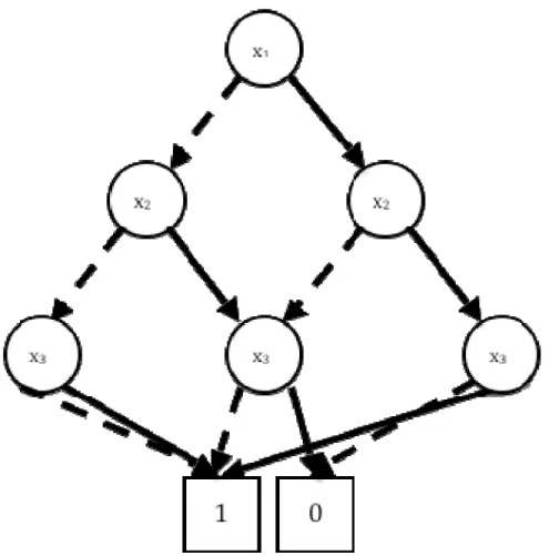
Figure 4. BDD with all isomorphic sub-graphs merged. ...21
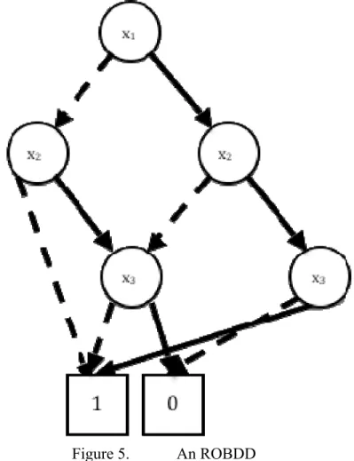
Figure 5. An ROBDD...22
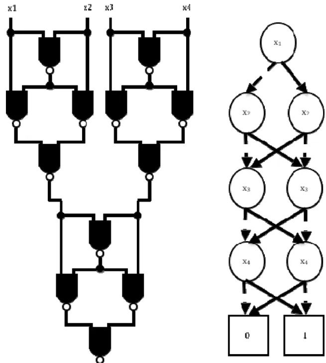
Figure 6. Side-by-side comparison of 4-variable XOR function as represented by Boolean circuit logic and a Binary Decision Diagram ...24
Figure 7. Minimum realization of DQF x1x2x3x4x5x6x7x8...27
Figure 8. Maximum realization of DQF x1x2x3x4x5x6x7x8. ...28
Figure 9. Comparison of BD Machine Code and Microprocessor Machine Code [15]..29
Figure 10. Creation of a QDD (labeled as MDD) from a minimized BDD [From 3]...31
Figure 11. Partial binary decision tree constructed by parsing a truth table. ...36
Figure 12. Partial BDD showing reduction of redundant node at level 3. ...37
Figure 13. ROBDD generated by parsing truth tables and merging identical sub-functions...38
Figure 14. DQF Order 2, AKA the AND Function of two variables. ...48
Figure 15. DQF Order 4 generated from concatenation of two disjoint AND functions...49
Figure 16. Partial Symmetric Bent Function Example...52
Figure 17. The mid-section of a symmetric bent BDD. ...53
Figure 18. x1x2x3x1x2x5x1x2x6x1x3x4 x1x3x5x1x4x5x1x4x6x1x5x6 x2x3x4 x2x3x6x2x4x5x2x4x6x2x5x6x3x4x5x3x4x6x3x5x6 ...55 Figure 19. x1x2x3x1x2x4 x1x2x5 x1x3x4x1x3x6x1x4x5 x1x4x6x1x5x6 x2x3x4x2x3x5x2x3x6x2x4x6x2x5x6x3x4x5x3x5x6x4x5x6 ...56 Figure 20. x1x2x3x1x2x4 x1x2x5 x1x3x4x1x3x5 x1x3x6x1x4x6x1x5x6 x2x3x4x2x3x6 x2x4x5x2x4x6x2x5x6x3x4x5x3x5x6x4x5x6 ...58 Figure 21. x1x2x3x1x2x4 x1x2x5 x1x2x6x1x3x4x1x3x5x1x4x6x1x5x6 x2x3x4 x2x3x6x2x4x5x2x5x6x3x4x5x3x4x6x3x5x6x4x5x6 ...59 Figure 22. DQF of order 2 (x1x2)...95 Figure 23. Complement of DQF (x1x2 1). ...95 Figure 24. x1x2x1...96 Figure 25. x1x2x2 ...96 Figure 26. x1x2x1x2 ...97 Figure 27. DQF of Order 4 (x1x2x3x4). ...98 Figure 28. Complement of DQF (x1x2 x3x41)...98 Figure 29. x1x2x3x4x1...99 Figure 30. x1x2x3x4x2...99 Figure 31. x1x2x3x4x3...100
Figure 32. x1x2x3x4x4...100 Figure 33. x1x2x3x4x1x2 ...101 Figure 34. x1x2x3x4x1x3...101 Figure 35. x1x2x3x4x1x4...102 Figure 36. x1x2x3x4x2x3...102 Figure 37. x1x2x3x4x2x4...103 Figure 38. x1x2x3x4x3x4...103 Figure 39. x1x2x3x4x1x2 x3...104 Figure 40. x1x2x3x4x1x2 x4...104 Figure 41. x1x2x3x4x1x3x4 ...105 Figure 42. x1x2x3x4x2x3x4...105 Figure 43. x1x2x3x4x1x2 x3x4...106 Figure 44. DQF of Order 6 (x1x2x3x4x5x6)...107 Figure 45. Complement of DQF (x1x2 x3x4x5x6 1 ). ...108 Figure 46. x1x2x3x4x5x6x1...109 Figure 47. x1x2x3x4x5x6x2 ...110 Figure 48. x1x2x3x4x5x6x3 ...111 Figure 49. x1x2x3x4x5x6x4 ...112 Figure 50. x1x2x3x4x5x6x5 ...113 Figure 51. x1x2x3x4x5x6x6 ...114 Figure 52. x1x2x3x4x5x6x1x2...115 Figure 53. x1x2x3x4x5x6x1x3...116 Figure 54. x1x2x3x4x5x6x1x4 ...117 Figure 55. x1x2x3x4x5x6x1x6...118 Figure 56. x1x2x3x4x5x6x2x4 ...119 Figure 57. x1x2x3x4x5x6x3x6 ...120 Figure 58. x1x2x3x4x5x6x1x2x3...121 Figure 59. x1x2x3x4x5x6x2x3x4 ...122 Figure 60. x1x2x3x4x5x6x3x4 x5 ...123 Figure 61. x1x2x3x4x5x6x2x3x4x5 ...124 Figure 62. x1x2x3x4x5x6x1x2x3x4 x5 ...125 Figure 63. x1x2x3x4x5x6x2x3x4x5 x6...126 Figure 64. x1x2x3x4x5x6x1x2x3x4 x5x6 ...127 Figure 65. Order 8 DQF (x1x2 x3x4x5x6x7x8)...128 Figure 66. x1x2x3x4x5x6x7x8 x1...129 Figure 67. x1x2x3x4x5x6x7x8 x2...130
Figure 71. Symmetric Bent Function of Order 2 (x1x2)...135
Figure 72. Symmetric Bent Function of Order 4...136
Figure 73. Symmetric Bent Function of Order 6...137
Figure 74. Symmetric Bent Function of Order 8...138
Figure 75. x1x2x3x1x2x5x1x2x7x1x2x8x1x3x8x1x4x6 x1x4x8 x1x5x6 x1x7x8x2x3x5x2x3x6x2x3x7 x2x5x6x2x5x8 x3x4x7x3x4x8 x3x5x7 x3x6x7x4x5x6x4x5x7x4x6x7x4x6x8x4x7x8x5x6x8 ..139 Figure 76. x1x2x6x1x2x8x1x3x4 x1x3x8x1x4x5x1x4x7x1x4x8x1x5x6 x1x7x8x2x3x7 x2x3x8 x2x5x6x2x5x7x2x6x7 x2x6x8x2x7x8 x3x4x5x3x4x6x3x4x7x3x5x7x3x6x7x4x5x6x4x5x8x5x6x8 .140 Figure 77. x1x2x3x1x2x5x1x2x6x1x2x8x1x3x5x1x3x6x1x3x7x1x4x7 x1x4x8 x1x5x7x1x5x8x1x6x7x1x6x8x2x3x5x2x3x7x2x3x8 x2x5x6x2x5x7 x3x4x6x3x4x7x3x5x6x3x5x8x3x6x8x3x7x8 x4x5x6x4x5x8x4x6x7x4x6x8x4x7x8x5x6x7x5x7x8x6x7x8 .141 Figure 78. x1x2x3x1x2x5x1x2x6x1x2x8x1x3x7x1x4x7 x1x4x8x1x5x8 x1x6x8x2x3x5x2x3x7x2x3x8x2x5x6x2x5x7 x3x4x6x3x4x7 x3x5x6x3x7x8 x4x5x6 x4x5x8 x4x6x7 x4x6x8 x4x7x8x5x6x7 ..142 Figure 79. x1x2x7x1x2x8x1x3x4 x1x3x7x1x4x5x1x4x6x1x4x8 x1x5x8 x1x6x8x2x3x6x2x3x7x2x5x6x2x5x8x2x6x7x2x6x8 x2x7x8 x3x4x5x3x4x7 x3x4x8x3x5x6x3x7x8x4x5x6x4x5x7x5x6x7 .143 Figure 80. x1x2x7x1x2x8x1x3x4 x1x3x5x1x3x6x1x3x7 x1x4x5x1x4x6 x1x4x8x1x5x7x1x5x8x1x6x7x1x6x8x2x3x6x2x3x7x2x5x6 x2x5x8x2x6x7 x2x6x8x2x7x8x3x4x5x3x4x7x3x4x8x3x5x6 x3x5x8x3x6x8x3x7x8x4x5x6 x4x5x7x5x6x7x5x7x8x6x7x8 .144 Figure 81. x1x2x6x1x2x8x1x3x4 x1x3x5x1x3x6x1x3x8x1x4x5x1x4x7 x1x4x8x1x5x6x1x5x7x1x6x7x1x7x8x2x3x7x2x3x8x2x5x6 x2x5x7x2x6x7x2x6x8x2x7x8x3x4x5x3x4x6x3x4x7 x3x5x7 x3x5x8x3x6x7 x3x6x8x4x5x6 x4x5x8 x5x6x8x5x7x8x6x7x8 .145 Figure 82. x1x2x3x1x2x5x1x2x7x1x2x8x1x3x5x1x3x6 x1x3x8x1x4x6 x1x4x8 x1x5x6x1x5x7x1x6x7x1x7x8x2x3x5x2x3x6x2x3x7 x2x5x6x2x5x8x3x4x7x3x4x8 x3x5x7x3x5x8x3x6x7x3x6x8 x4x5x6x4x5x7x4x6x7 x4x6x8 x4x7x8 x5x6x8x5x7x8x6x7x8 .146 Figure 83. Hex Truth Table: 00110572175C476A 032E357E1B6C7869 00775F4E173AE2A9 3F74AC81D8C9E196...147
Figure 84. Hex Truth Table: 01041576134C526B 023B257A1F7C6D68 15760E0B526BE3BC 2A75FDC49D98E083 ...148
Figure 85. Hex Truth Table: 01150713105E703E 071C68737F3E89C8 077A68157F5889AE 67EA61EC76A116C1 ...149
Figure 86. Hex Truth Table: 0017051212367E5A 170F746C5F74AA9 1173C476C5FB8668 133E8FA21DEC98196...150
LIST OF TABLES
Table 1. Truth table for the three variable exclusive-or function. The column
underneath f represents the truth table of the Boolean function. ...3
Table 2. Known bent function quantities (After [2]). ...11
Table 3. Condensed Truth Table of an Arbitrary Four-Variable Symmetric Function ...12
Table 4. Full Truth Table of the same Four-Variable Symmetric Function ...13
Table 5. Condensed Truth Table of the Basic Form of a Symmetric Bent Function...14
Table 6. Maximum complexity (number of nodes) in a BDD representative of a Boolean function of n-variables...25
Table 7. Arbitrary 4-variable function split into sub-functions ...35
Table 8. Application of Johnson-Trotter Algorithm to generate all possible variable orderings of a 4-variable function...42
Table 9. Swapping variables x1 and x2 will result in the manipulation of the highlighted truth table entries. ...43
Table 10. Swapping variables x2 and x3 in an arbitrary 4-variable function...44
Table 11. Swapping variables x3 and x4 in an arbitrary 4-variable function...45
Table 12. Number of Non-Terminal Nodes in the BDD of DQFs...48
Table 13. Condensed Truth Table of a Symmetric Bent Function. ...50
Table 14. The Number of Non-Terminal Nodes in the BDDs of Symmetric Bent Functions...51
EXECUTIVE SUMMARY
Bent functions are Boolean functions that have a maximum Hamming distance from the linear functions and their complements – otherwise known as the affine functions. That is, bent functions have maximum nonlinearity. High nonlinearity is a desirable property for functions used in cryptographic applications because it hardens the cryptographic system from linear cryptanalysis attacks.
Another useful aspect of bent functions in terms of cryptography is that they are rare and difficult to find. While this increases their security, this is also frustrating because this makes them difficult to research. Many known sets of bent function families can be designed generally for a function of n-variables, but the vast majority must be found through enumeration of all Boolean functions. For this reason, identifying the characteristics of bent functions from a variety of perspectives may prove valuable in unlocking methods of more efficient discovery.
One method for representing a Boolean function is with a Reduced Ordered Binary Decision Diagram (ROBDD, or BDD, for short). BDDs are tree-like graph structures that provide a condensed form of the function that can be traversed one variable at a time. Complex functions can be calculated fairly quickly with BDDs, which makes them desirable for real-time and computer aided design applications.
It is known that for many human designed Boolean functions, BDDs tend to have simple shapes. This is likely because functions with simple characteristics are useful. Good examples of simple but useful functions are the AND, OR, and XOR functions, which have simple BDDs.
On the other hand, no one has looked closely at the BDDs of known bent functions. Due to their nonlinearity, it is expected bent functions would have high complexity in relation to other human designed functions. Furthermore, little is known about how the shape of bent function BDDs or how the BDDs of different types of bent functions may be related.
This thesis explores the BDDs of bent functions. Since BDD construction can be quite time consuming by hand, the first step was to create a program capable of generating a BDD given the truth table of a Boolean function. Although many programs are available that can convert a function into a BDD data structure, there are none known that integrate a graphical display of the BDD. Creating a program to aid in the visualization necessary was the first order of business.
BDD complexity can also be very sensitive to variable ordering. For instance, one variable ordering of an 8-variable Disjoint Quadratic Function results in a BDD with 14 nodes, while another “diabolical” ordering results in a BDD with 37 nodes. Since in almost all cases, a minimized BDD is desirable, the program had to be able to implement a method for permuting variables in order to find trees of a minimum size.
Designing this program, called BDDViewer, resulted in the realization that the BDD can be fully implemented by parsing the function’s truth table. Specifically, the edges of each node split the truth table in half, with each node representing a sub-function. By viewing each node as a unique sub-function’s truth table, an ROBDD can be constructed with no redundant, or isomorphic sub-graphs.
By implementing the BDD construction in this way, the variable order permutations also had to be properly reflected in the corresponding truth table. The Johnson-Trotter permutation algorithm was used to find all possible variable orderings. However, a new algorithm was developed to manipulate the truth table to reflect the movement of the variables. The details of this algorithm can be seen in Chapter IV.
Once the program was complete, the BDDs of a sampling of known bent functions were investigated. Specifically, disjoint quadratic functions (DQFs), symmetric bent functions, and homogeneous functions of algebraic degree 3 on 6-variables were observed. XORing these functions with linear functions was also performed to identify bent functions’ relationship with their affine classes.
the minimum BDDs of DQFs were found to have 2n – 2 non-terminal nodes, while the
minimum BDDs of symmetric bent functions were found to have 4n – 8 non-terminal
nodes. Furthermore, the simple observation of the BDDs of the symmetric bent function demonstrates the cyclic nature of symmetric functions. Specifically, the functions are dependent entirely on the number of variables set to 1, and not the order in which the variables are listed.
The BDDs of the homogeneous functions of 6-variables, while not nearly as aesthetically pleasing as the DQFs and symmetric bent functions, were still quite revealing. All 30 functions were revealed to have identical BDD structures. That is, the total number of nodes per level in each BDD was identical. From this realization, it was discovered that P-equivalent functions will have identical BDDs for distinct variable orderings.
Finally, the BDDs of functions in the same affine class were shown to have identical structures. Functions in the same affine class are not P-equivalent, so the BDDs themselves were not identical, but this discovery demonstrated that all functions in an affine class have BDDs of the same size.
The research demonstrated that many bent functions, despite their nonlinearity, have predictable characteristics. However, only a small sample of bent functions was investigated. Further research may yield more comprehensive results. The creation of a program capable of finding the minimum BDD of any Boolean function may also prove broadly useful to others interested in BDD construction.
I. INTRODUCTION
A. PROBLEM DEFINITION
Most modern cryptographic systems rely on Boolean functions as a part of the cipher process. In order to be effective, these Boolean functions must exhibit certain properties that aid in the obfuscation of the cryptographic key to an attacker. Amongst other properties, such as balancedness or low autocorrelation, ciphers benefit from Boolean functions with a high nonlinearity.
Boolean bent functions have the unique property of having the highest nonlinearity for any given function of n-variables [1]. Bent functions are also extremely rare and difficult to enumerate, making the discovery of unique bent functions for large n
quite valuable. Despite their nonlinearity, bent functions alone do not make cryptographically sound Boolean functions, because they lack balancedness. However, bent functions make an excellent starting point for modification into a cryptographically sound Boolean function [2].
One method of representing a Boolean function is through a Reduced Ordered Binary Decision Diagram (ROBDD, or BDD for short). In a binary decision diagram, the function is represented graphically in a binary tree structure. Each level of the tree corresponds to a variable of the function, and each edge between vertices represents the decision of either a binary 0 or 1 for that variable. Thus, by setting each input variable to either a 0 or 1, the tree can be traversed, revealing the output of the function for that specific combination of input variables. BDDs can be useful because many human-designed functions have simple BDDs. That is, they tend to have a relatively small number of vertices, or nodes. Representing a function in this manner can result in speedy computation of functions, or reveal interesting characteristics when viewed graphically [3].
B. THESIS GOALS
This thesis analyzes a subset of well-known bent functions with the intention of identifying their characteristics with regard to their respective binary decision diagrams. This approach is taken because bent functions are inherently complex, and it is believed that research of this nature has never been attempted.
In particular, disjoint quadratic functions, homogeneous bent functions of algebraic degree three, and symmetric bent functions are analyzed in depth. Where applicable, patterns in these functions’ structures are commented upon, and observations on the minimum size and characteristics of these functions are discussed.
An additional goal of this thesis is to develop a graphical program that displays an easily readable binary decision diagram of any given function. This program will be useful for future research projects on the topic of binary decision diagrams.
C. THESIS ORGANIZATION
Chapter I focuses on the general overview of the problem and presents the goal of the thesis. Chapter II provides background on Boolean functions, as well as defining bent functions and introducing the difficulties in enumerating those functions. Chapter III discusses binary decision diagrams in greater detail, indicating their current and future applications. Chapter IV describes the program used in this thesis to model the binary decision diagrams, and touches on algorithms that may be relevant to future researchers. Chapter V analyzes the binary decision diagrams of a subset of the known bent functions. Chapter VI summarizes the findings of Chapter V and discusses improvements that can be implemented on the program designed for this thesis as well as future research that can be attempted on binary decision diagrams of bent functions and functions with other cryptographic properties.
II.
BOOLEAN FUNCTIONS AND THEIR CRYPTOGRAPHIC
PROPERTIES
A. BOOLEAN FUNCTIONS
A Boolean function f of n variables is defined as f :2
n
2,2
0,1 ,where 2n represents the vectorspace of dimension n of the binary field
2 [2]. Boolean
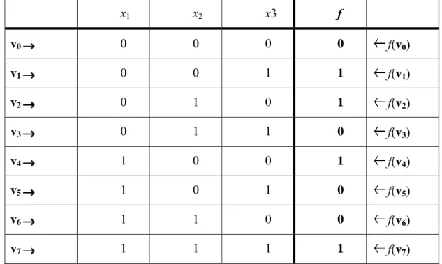
functions are commonly represented by a truth table, which represents the (0,1) value for each combination of n input variables, each also set to (0,1). In other words, the truth table is the (0,1) sequence defined by (f(v0), f(v1),…, f(v2^(n-1))) where v0 represents the n
variables defined as (0,…0,0), v1 = (0,…0,1), and v2^(n-1) = (1,…1,1), ordered
lexicographically [2]. This paper will often refer to a truth table simply as TT.
x1 x2 x3 f v0 0 0 0 0 f(v0) v1 0 0 1 1 f(v1) v2 0 1 0 1 f(v2) v3 0 1 1 0 f(v3) v4 1 0 0 1 f(v4) v5 1 0 1 0 f(v5) v6 1 1 0 0 f(v6) v7 1 1 1 1 f(v7)
Table 1. Truth table for the three variable exclusive-or function. The column underneath f
1. Algebraic Normal Form
Boolean functions can also be represented in Algebraic Normal Form (ANF), a standardized method for representing Boolean functions. Functions represented in this form have the benefit of allowing one to identify its linear characteristics more readily than its truth table form. A Boolean function f of n variables can be represented in ANF as f(x1,x2,...,xn)a0 a1x1a2x2 anxn a1,2x1x2an1,nxn1xn a1,2,...,nx1x2xn,
where the coefficients ai
0,1 . In the previous example of a three variable exclusive-or function, the coefficients a1=a2=a3=1, and all other coefficients ai = 0. Thus, the ANF ofthe exclusive-or function is
f(x1,x2,x3)1x11x21x3 x1x2 x3.
2. Algebraic Degree
The algebraic degree of a Boolean function is the number of variables in the highest order monomial of the ANF with a nonzero coefficient [2]. In the function
f x1x2x3x4x5
the algebraic degree is 3 due to the monomial x3x4x5.
3. Linear Functions
A linear function is any function of algebraic degree one and for which a0=0. The notation for a linear function is commonly given as
4. Affine Functions
Affine functions are all of the linear functions and their complements. Affine functions can be written as
a,c(x)axc,
where c
0,1 [2]. Note that the constant functions 0 and 1 are both considered affine functions.5. Hamming Weight
The Hamming weight, denoted by wt(f), of a function f is the number of nonzero values in its truth table. For a Boolean function, the Hamming weight is simply the number of ones in the truth table. In the case of the exclusive-or function of three variables, the Hamming weight is 4, since there are four ones in the function, as shown in Table 1.
6. Hamming Distance
The Hamming distance between two functions is the number of truth table
elements that differ from each other. Between two functions f and g, the Hamming
distance can be defined as
d(f,g)wt(f g) [2]. B. CIPHERS
In order to stand up to a variety of cryptanalysis attacks, the Boolean functions used to generate a cryptographic key must satisfy several, often-conflicting properties. Properties that may help reduce vulnerability to one attack may not be useful against another. Before going on, a few definitions:
1. Plaintext
Plaintext in a cryptography scheme represents the raw information or data that a user intends to transmit. Plaintext has not yet been altered by an encryption process.
2. Cryptographic Key
The cryptographic key is the parameter that modifies the plaintext to generate an encrypted ciphertext. Generally, keys should be large enough such that the key cannot be guessed by an attacker through enumeration, or brute force. An example of a cryptographic key is the 256-bit key assigned by a user of Wi-Fi Protected Access / Pre-shared Key (WPA2/PSK) in many wireless networks.
3. Ciphertext
Ciphertext is the output of a cryptographic process after a cryptographic key has been used to modify the original plaintext data.
4. Cipher Example
In order to demonstrate the application of a key to generate ciphertext, a simple stream cipher will be discussed.
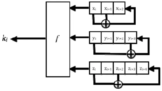
Figure 1. A simple cipher using a 12-bit key.
Since linear feedback shift registers (LFSRs) are easy and cheap to implement, they are frequently used in pseudo-random key generators. In Figure 1, a 12-bit key is spread amongst three “x” bits, four “y” bits, and five “z” bits. The XOR functions shown
function applied to each of the incoming stream of bits. This function f could be as simple as an XOR operation, but generally a more cryptographically secure Boolean function is chosen. The output, ki, is then combined with a plaintext bit, typically via an XOR
operation to generate one bit of ciphertext. The LFSRs compute the next series of bits in the keystream and the process is repeated until all plaintext has been encrypted. In order for the receiver to decrypt the ciphertext into a plaintext form, knowledge of the function
f, the LFSR patterns, and the initial bits in the keystream must be known. These are the aspects of a cipher for which cryptographically secure properties are desirable.
5. Cryptographic Properties
When constructing a cryptographic system, the cipher’s primary characteristics should be to create diffusion and confusion. Diffusion helps to mask the key and the plaintext data by dissipating the statistical properties of the ciphertext. In other words, each bit of the cipher function should affect as many bits of the plaintext as possible to spread the statistical significance of each bit in the ciphertext over a wide range. Ideally, for every bit change in the plaintext, a good cipher would change exactly half of the bits in the final cipher text, making the structure of the plaintext more difficult to detect [4, 5].
Confusion, as described by Claude Shannon, is “the method to make the relation between the simple statistics of the ciphertext and the simple description of the key a very complex and involved one.” Ultimately, the goal of a confusing cipher is to make it difficult to identify the encryption key even if multiple ciphertext-plaintext pairs have been identified.
In general, properties identified as useful for cryptographic purposes are balancedness, low autocorrelation, correlation immunity, algebraic immunity, and nonlinearity. The majority of these properties will not be defined here, as they are not particularly relevant to the research conducted for this thesis, which will focus on the very desirable property of nonlinearity, specifically in regard to the study of bent functions. However, extensive studies have been done on the other cryptographic properties mentioned by other researchers, and the reader is directed to [2] and the references therein for further information.
It is worth mentioning that tradeoffs are required for any cryptographic function, as no Boolean function can exemplify all of the cryptographic properties. For example, bent functions, which have maximum nonlinearity, are never balanced. Balanced functions are those that contain an equal number of 1s and 0s in their truth tables, and help satisfy the cryptographic property of diffusion. Since bent functions can never be balanced [1, 2], a bent function is rarely used in an encryption device. It is possible, instead, to modify a bent function such that it becomes balanced, at some cost to its nonlinearity.
C. BENT FUNCTIONS
As previously mentioned, bent functions are those that have the highest possible nonlinearity for a function of n-variables. That is, bent functions have the highest possible Hamming distance from the affine functions of n-variables. This property of nonlinearity is important in generating confusion in a cryptographic process, since linear cryptanalysis attacks are capable of breaking most highly linear systems easily by using an affine function to approximate the actual function used [6]. For this reason, bent functions are useful in the generation of cryptographic ciphers.
1. Definitions a. Nonlinearity
In a paper by Butler and Sasao [7], nonlinearity is succinctly defined as: The nonlinearity NLf of a function f is the minimum number of truth table
entries that must be changed in order to convert f to an affine function.
Nonlinearity can also be defined as the minimum Hamming distance between the truth tables of f and an affine function.
NLf min(wt(f a1),wt(f a2),...,wt(f ak)), where aiis an affine function indexed by 1 ≤i≤k = 2n+1.
The 3-variable function f =x1x2x3 has a nonlinearity of 1. The AND
function f has a solitary 1 in its truth table, which has a Hamming distance of 1 from the linear function of constant 0, and of course, f is not itself affine [7].
b. Bent Functions
Let f be a Boolean function on n-variables, where n is even. f is a bent function if its nonlinearity is 2n12
n
21
[7].
Bent functions can also be defined by their Walsh transform coefficients. Specifically, a Boolean function f in n variables is called bent if and only if the Walsh transform coefficients of f^ are all ±2n/2, that is, W(f^)2
is constant. f^ represents the sign function of function f, and W() is the Walsh transform [2]. This definition is useful when using bent functions in spread spectrum applications. This definition in terms of Walsh transform coefficients is only offered here for completeness; for the sake of this thesis, nonlinearity is the primary concern.
2. The Difficulty of Discovering Bent Functions
Despite bent functions’ inherent usefulness in cryptographic applications, they are notoriously difficult to find. Although there are a few well-known classes of bent function that can be constructed for any number of n-variables, the majority of functions can only be found through computational enumeration. That is, the truth table of every function of n-variables must be sequentially checked against the known affine functions for nonlinearity. This process is time consuming, as there exist 22n
functions to compare! Even for the relatively small set of Boolean functions of 6-variables, there exist1.841019
functions to enumerate in search for the entire set of bent functions! Complicating matters further, the number of bent functions of n-variables is
unknown for general n. Upper and lower bounds have been identified, but the exact
a. Lower Bound
It has been shown by [8, 2] that rows in the Sylvester-Hadamard matrix yield a bent function when concatenated. The definition of the Sylvester-Hadamard matrix and the derivation of the findings are beyond the scope of this thesis. Nevertheless, it has been shown that, for n = 2k, the concatenation of the 2k Sylvester-Hadamard rows or their complements in arbitrary order results in (2k)!22k
different bent functions of n-variables [8, 2]. Thus, there exist at least (2k
)!22k
bent functions for n = 2k
variables.
b. Upper Bound
In [1] it was shown that the maximum algebraic degree of a bent function is n/2 for n > 2. This implies that the algebraic normal form has
n i i0 n/2
2n11 2 n n/ 2 coefficients,any of which can be either 0 or 1 [2], while all other coefficients must be 0. Thus, the number of functions that can be derived from these coefficients is
22 n11 2 n n/2 ,
which represents the upper bound of total possible bent functions of n-variables.
c. Enumerations
Due to the difficulties described in identifying the truth table or even the total number of bent functions, the total set of bent functions is only known up to 8-variables. Although bent functions are cryptographically desirable due to their nonlinearity, they have the added benefit of being rare and difficult to find. The lack of knowledge of higher order functions makes their employment particularly useful. Still, the following chart should illuminate the difficulties in discovering a bent function.
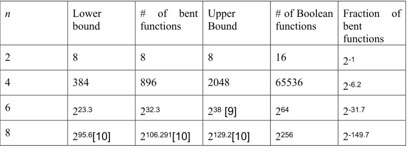
n Lower bound # of bent functions Upper Bound # of Boolean functions Fraction of bent functions 2 8 8 8 16 2-1 4 384 896 2048 65536 2-6.2 6 223.3 232.3 238 [9] 264 2-31.7 8 295.6[10] 2106.291[10] 2129.2[10] 2256 2-149.7
Table 2. Known bent function quantities (After [2]).
Table 2 helps to illustrate the difficulties described above. For instance, there are 2256 1.1581077 Boolean functions of 8-variables. Assuming that a 2.4GHz
computer could identify a function as bent or not at the rate of one function per clock cycle, it would still take 1.531060 years to search the entire solution-space. It is for this
reason that the bent functions are relatively unknown for n ≥ 10. Furthermore, it is significant to note that, as the number of variables increases, the proportion of bent functions as compared to the total number of Boolean functions decreases quite rapidly. This makes the short-term yield of sequential or random enumeration of Boolean functions in an effort to exhaustively search quite low.
3. Known Bent Functions
Even though bent functions are extraordinarily difficult to find within the total search space, there are many known classes that can be constructed for any order n -variables. A few of those classes will be discussed here.
a. Disjoint Quadratic Functions
Disjoint Quadratic Functions (DQFs) are functions of the form
f(x1,y1,...,xk,yk) i1xiyi x1y1x2y2 xkyk
k
and were shown in Rothaus’ original paper to be bent [1]. Rothaus called these functions members of FAMILY I, and are considered the simplest general form of bent functions
[11]. FAMILY I bent functions are also called the dot product, and can be written as
f(x,y)xy.
FAMILY II bent functions are related in that they are a DQF concatenated with any function of half the variable set. That is, FAMILY II functions can be written as
f(x,y)xyg(x) or f(x,y)xyg(y) ,
where g is any arbitrary function. Note that g must be composed specifically of the variables associated with x or the variables associated with y and cannot be mixed [1, 11].
b. Symmetric Bent Functions
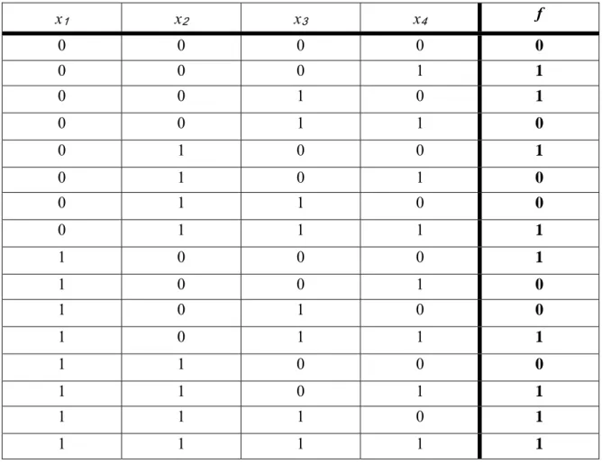
A symmetric Boolean function is unchanged by any permutation of the input variables. An example of a symmetric function is the AND operation. Regardless of the ordering of the variables, the truth table will always be {0,0,0,1}. Due to dependence of symmetric functions on only the number of variables set to 1, symmetric functions can be represented in a condensed truth table. Tables 3 and 4 serve to illustrate this property. Note specifically how the number of variables column of Table 3 corresponds with the output value in both tables.
# of Variables set to 1 f 0 0 1 1 2 0 3 1 4 1 Table 3. Condensed Truth Table of an Arbitrary Four-Variable Symmetric Function
x1 x2 x3 x4 f 0 0 0 0 0 0 0 0 1 1 0 0 1 0 1 0 0 1 1 0 0 1 0 0 1 0 1 0 1 0 0 1 1 0 0 0 1 1 1 1 1 0 0 0 1 1 0 0 1 0 1 0 1 0 0 1 0 1 1 1 1 1 0 0 0 1 1 0 1 1 1 1 1 0 1 1 1 1 1 1
Table 4. Full Truth Table of the same Four-Variable Symmetric Function
Bent functions that are also symmetric are interesting in that there are only four possible functions [12], regardless of the number of variables. All symmetric bent functions have the form
f(x1,x2,...,xn) xixjc xid i1 n
1
ijn ,where c,d
0,1 . The four different functions result from the four assignments of values to c and d.In the simplest case, both c and d are set to 0, resulting in the symmetric bent function of the form
f(x1,x2,...,xn) xixj x1x2x1x3x1xn x2x3 1
ijnxn1xn.
This form is the XOR operation on all possible pairs of variables. Since the XOR operation results in 1 only when there are an odd number of product terms of value 1, it has been proven previously that the condensed truth table of the function takes the form
ck k 2
mod 2
,where ck is the output of the condensed truth table for k variables set to 1 [2]. Table 5
illustrates the pattern the condensed truth table follows, namely as the variables set to 1 increases incrementally, the condensed truth table follows the repeating pattern {0, 0, 1, 1}. Thus, a truth table can be constructed for a symmetric bent function of any size of n -variables. # of Variables set to 1 f 0 0 1 0 2 1 3 1 4 0 5 0 6 1 7 1
c. Constructing Bent Functions
In addition to general forms of bent functions that can be constructed for functions of any size, some methods exist for constructing new bent functions from known bent functions.
(1) Concatenation. Given a function f(x) and g(y) that are both bent, the concatenation h(x,y) f(x)g(y) is also bent [2]. Note that x and y are disjoint sets of variables. Thus, if f(x) and g(y) are each 4-variable functions, the resulting function h(x,y)is an 8-variable function.
(2) Affine Classes. Given a bent function f, the XORof f and any affine function on the same set of variables is also bent. That is, g(x) f(x)(x) is bent if f is bent and is affine [2]. It should be noted that g(x) is considered to be in the same affine class as f(x).
D. SUMMARY
In this chapter, Boolean bent functions were defined. Bent functions are valuable in cryptographic systems due to the protection they offer against linear cryptanalysis attacks. However, bent functions are rare and difficult to find. Since the binary decision diagrams (BDDs) of bent functions have never been specifically investigated, the next chapter will focus on the construction, characteristics, and applications of BDDs.
III. BINARY
DECISION
DIAGRAMS
There are many methods for representing a Boolean function. The most common are truth tables, as discussed in Chapter II, and circuits. Circuit representation uses transistor gates to model the function in digital form. Truth tables are typically used in the design phase to identify characteristics of the function, and the circuit representation is used in the implementation of the function, such as in an integrated circuit or Field Programmable Gate Array (FPGA).
Another practical method of representing a Boolean function is by a Binary Decision Diagram (BDD), which organizes the function into a tree structure that can be traversed one variable at a time. Representing functions in this form is currently popular in many Computer Aided Design (CAD) applications [15]. The remainder of this chapter will describe the construction of BDDs and their valuable properties.
A. BINARY DECISION DIAGRAM CONSTRUCTION
In a BDD, a Boolean function is represented as a rooted, directed, acyclic graph in which each vertex, or node, has two edges, or links. Each node represents a variable (i.e.,
x1, x2, etc) and each edge represents a decision for that variable. Specifically, the edge represents either a 0 or 1 decision in the tree. Thus, the 0 edge for a node representing x2
symbolizes the sub-function for which input variable x2 is set to 0.
Typically, operations are performed on the BDD to reduce its complexity while still maintaining its canonical representation of the originating Boolean function. For clarity, this thesis will first describe BDDs for which no reductions are performed.
1. Binary Decision Tree
Although technically not considered a BDD, decision trees represent the simplest method of converting a Boolean function to a tree structure. A decision tree is a full, complete binary tree, meaning that each level of the tree is filled, and each node has two children. In other words, every binary decision tree of n-variables will have 2n 1