ST-Hadoop: A MapReduce Framework for Big Spatio-temporal Data Management

(1)

ST-Hadoop: A MapReduce Framework for Big

Spatio-temporal Data Management

A DISSERTATION

SUBMITTED TO THE FACULTY OF THE GRADUATE SCHOOL OF THE UNIVERSITY OF MINNESOTA

BY

Louai Alarabi

IN PARTIAL FULFILLMENT OF THE REQUIREMENTS FOR THE DEGREE OF

Doctor of Philosophy

Mohamed F. Mokbel

(2)

(3)

Acknowledgements

There are many people have earned my gratitude for their contribution and involve-ment to my success in graduate school, including my parents, siblings, spouse, children, doctoral adviser, examination committees, friends, colleagues, and sponsor.

I am incredibly thankful to Prof. Mohamed F. Mokbel for his guidance throughout my stay in graduate school. I want to express my sincere gratitude for his generous support. I consider myself highly fortunate to work with him closely. I always have been inspired by his passion and commitment toward research and building systems. I would not have become the scientist that I am today without his wisdom and assistance, I have grasped from him critical thinking and hard working.

Besides the primary adviser, I am grateful to Prof. Shashi Shekhar, Prof. Steven M Manson, Prof. Jon Weissman, and Prof. Abhishek Chandra for serving on my preliminary and thesis committee. Very appreciative for their essential and constructive feedback that shaped my final dissertation. I am thankful to Prof. Shashi Shekhar for his insightful comments and for sharing with me his tremendous experience in the spatial data management field. I am grateful to Prof. Steven Manson for his insightful comments and for sharing his expertise in geographic information science all the way through my Master and Ph.d program. I am thankful to Prof. Jon Weissman, and Prof. Abhishek Chandra for their profound insight and knowledge in distributed frameworks. I am grateful to Dr. Shana Watters for sharing with me her teaching experience and being a role model. I am very thankful for her encouragement. I sincerely appreciate all skills they imparted to my academic and professional life.

I am very thankful to Prof. Saleh M. Basalamah for his strong support and recom-mendation to join Prof. Mokbels research group. I want to express my sincere appre-ciation to (UQU) UMM AL-Qura University for their generous sponsorship during the

(4)

(NSF) the National Science Foundation, and Microsoft for their generous grants and financial support that otherwise I would not be able to share my scientific explorations and be actively engage in conferences.

I am so grateful for my supportive and motivating family. I am honored to be a son of a great man Mishal Alarabi, and wonderful mother Hanan Aqlan. I am very thankful to my parents for their unconditional support and believing in me. I am a proud brother to amazing siblings Lena, Wael, Walaa, Raied, and Raneem. I am genuinely indebted to my cheerleader wife, Mada Sabbah, for her unlimited support and countless sacrifices. Together, we celebrated every acceptance and moderated every rejection. Mada and my children Aseel, Zain and the little unborn ones are the joy of my life and the special blessing.

I would like to thank all members of Mokbel’s Lab, including alumni and current ones for making my experience in data management lab and grad school fun and exciting. In particular, Mohamed Sarwat, Abdeltawab Hendawi, Jie Bao, Ahmed Eldawy, Rami Alghamdi, Saif Al-Harthi, Christopher Jonathan, Mashaal Musleh, Ibrahim Sabek, Har-shada Chavan, Bin Cao, Prof. Kwang Woo Nam, Xiaochuang Yao, and Rana Forsati.

(5)

Dedication

To those who held me up over the years. Thank you.

(6)

Abstract

Apache Hadoop, employing the MapReduce programming paradigm, that has been widely accepted as the standard framework for analyzing big data in distributed en-vironments. Unfortunately, this rich framework was not genuinely exploited towards processing large-scale spatio-temporal data, especially with the emergence and popular-ity of applications that create them in large-scale. The huge volumes of spatio-temporal data come from applications, like Taxi fleet in urban computing, Asteroids in astronomy research studies, animal movements in habitat studies, neuron analysis in neuroscience research studies, and contents of social networks (e.g., Twitter or Facebook). Managing space and time are two fundamental characteristics that raised the demand for process-ing spatio-temporal data created by these applications. Besides the massive size of data, the complexity of shapes and formats associated with these data raised many challenges in managing spatio-temporal data.

The goal of dissertation is centered on establishing a full-fledged big spatio-temporal data management system that serves the need for a wide range of spatio-temporal ap-plications. This involves indexing, querying, and analyzing spatio-temporal data. We propose ST-Hadoop; the first full-fledged open-source system with a native support for

big spatio-temporal data, available to downloadhttp://st-hadoop.cs.umn.edu/.

ST-Hadoop injects spatio-temporal data awareness inside the highly popular ST-Hadoop system

that is considered the state-of-the-art for oﬀ-line analysis of big data systems.

Consider-ing a distributed environment, we focus on the followConsider-ing: (1) indexConsider-ing spatio-temporal data and (2) Supporting various fundamental spatio-temporal operations, such as range,

kNN, and join. Throughout this document, we will touch base on the background and

related work, motivate for the proposed system, and highlight our contributions.

(7)

List of Tables

2.1 Existing Work in the area of Big Spatial data . . . 18

2.2 Existing Work in the area of Big Spatio-temporal data . . . 19

4.1 Twitter Datasets . . . 33

4.2 ST-Hadoop Experiments Parameters . . . 34

7.1 New York Taxi and Limousine Dataset . . . 92

7.2 Summit Experiments Parameters Settings . . . 92

(11)

List of Figures

1.1 Range query in SpatialHadoop vs. ST-Hadoop . . . 2

3.1 ST-Hadoop system architecture . . . 21

4.1 HDFSs in ST-Hadoop VS SpatialHadoop . . . 24

4.2 Indexing in ST-Hadoop . . . 27

4.3 Data-Slice . . . 29

4.4 Time-Slice . . . 30

4.5 Temporal Hierarchy Index . . . 32

5.1 Landscape of spatio-temporal kNN operation . . . 40

5.2 Correctness check Final Answer . . . 41

5.3 Correctness Check when 0≤α≤1 . . . 42

5.4 Refinement Final Answer . . . 44

5.6 Range Query VS Input files (TB) . . . 48

5.7 Range Query VS Block size (MB) . . . 49

5.8 Range query with Block size VS Slicing ratio (α) . . . 50

5.9 The execution of kNN query on diﬀerent input files . . . 51

5.10 kNN query with various k . . . 51

5.11 kNN throughput while varying (α) of Ranking Function . . . 52

6.1 Conceptual representation of ST-Hadoop meta-data index . . . 55

6.2 Spatio-temporal Range Query Interval Window . . . 58

6.3 The eﬀect of the spatio-temporal query ranges on the best value of M . 59 6.4 ST-Hadoop Greedy query optimizer VS heuristicM . . . 60

7.1 Similarity query in ST-Hadoop vs. Summit . . . 63 ix

(12)

7.3 Temporal Slicing . . . 70

7.4 Trajectory Indexing . . . 71

7.5 Summit Trajectory Operations . . . 73

7.6 Local Computation: initial kanswer . . . 76

7.7 Correctness Check Cylinder . . . 79

7.8 MBR Trajectory distance . . . 81

7.9 Nearest Neighbor Trajectory-based in Summit . . . 83

7.10 Nearest Neighbor Trajectory-based correctness check . . . 84

7.11 Abstract idea of similarity computation in Summit . . . 88

7.12 Summit global computation of similarity query . . . 89

7.13 Range Query . . . 94

7.14 Summit stability . . . 96

7.15 kNN Query . . . 99

7.16 DTW similarity Query . . . 101

(13)

Chapter 1

Introduction

The importance of processing spatio-temporal data has gained much interest in the last few years, especially with the emergence and popularity of applications that create them in large-scale. For example, Taxi trajectory of New York city archive over 1.1 Billion trajectories [1], social network data (e.g., Twitter has over 500 Million new tweets every day) [2], NASA Satellite daily produces 4TB of data [3, 4], and European X-Ray Free-Electron Laser Facility produce large collection of spatio-temporal series at a rate of 40GB per second, that collectively form 50PB of data yearly [5]. Beside the huge achieved volume of the data, space and time are two fundamental characteristics that raise the demand for processing spatio-temporal data.

The current eﬀorts to process big spatio-temporal data on MapReduce

environ-ment either use: (a) General purpose distributed frameworks such as Hadoop [6] or

Spark [7], or (b) Big spatial data systems such as ESRI tools on Hadoop [8],

Parallel-Secondo [9], MD-HBase [10], Hadoop-GIS [11], GeoTrellis [12], GeoSpark [13], or

Spa-tialHadoop [14]. The former has been acceptable for typical analysis tasks as they organize data as non-indexed heap files. However, using these systems as-is will results in sub-performance for spatio-temporal applications that need indexing [15, 16, 17].

The latter reveal their ineﬃciency for supporting time-varying of spatial objects

be-cause their indexes are mainly geared toward processing spatial queries, e.g., SHAHED system [18] is built on top of SpatialHadoop [14].

Even though existing big spatial systems are eﬃcient for spatial operations,

nonethe-less, they suﬀer when they are processing spatio-temporal queries, e.g., ”find geo-tagged

(14)

Objects = LOAD’points’AS(id:int, Location:POINT, Time:t);

Result = FILTER ObjectsBY

Overlaps (Location,Rectangle(x1, y1, x2, y2)) AND t <t2 AND t >t1;

(a) Range query in SpatialHadoop

Objects = LOAD ’points’AS(id:int, STPoint:(Location,Time));

Result = FILTER Objects BY

Overlaps (STPoint,Rectangle(x1, y1, x2, y2), Interval(t1, t2) );

(b) Range query in ST-Hadoop

Figure 1.1: Range query in SpatialHadoop vs. ST-Hadoop

news in California area during the last three months”. Adopting any big spatial systems

to execute common types of spatio-temporal queries, e.g., range query, will suﬀer from

the following: (1) The spatial index is still illsuited to eﬃciently support time-varying of

spatial objects, mainly because the index are geared toward supporting spatial queries, in which result in scanning through irrelevant data to the query answer. (2) The system internal is unaware of the spatio-temporal properties of the objects, especially when they are routinely achieved in large-scale. Such aspect enforces the spatial index to be reconstructed from scratch with every batch update to accommodate new data, and thus the space division of regions in the spatial-index will be jammed, in which require more processing time for temporal queries. One possible way to recognize spatio-temporal data is to add one more dimension to the spatial index. Yet, such choice is incapable of accommodating new batch update without reconstruction the whole index from scratch.

This paper introduces ST-Hadoop; the first full-fledged open-source MapReduce framework with a native support for spatio-temporal data, available to download from [19]. ST-Hadoop is a comprehensive extension to Hadoop and SpatialHadoop that injects spatio-temporal data awareness inside each of their layers, mainly, index-ing, operations, and language layers. ST-Hadoop is compatible with SpatialHadoop and

(15)

3 program that deals with spatio-temporal data using ST-Hadoop will have orders of mag-nitude better performance than Hadoop and SpatialHadoop. Figures 1.1(a) and 1.1(b) show how to express a spatio-temporal range query in SpatialHadoop and ST-Hadoop, respectively. The query finds all points within a certain rectangular area represented by

two corner points⟨x1,y1⟩ ,⟨x2,y2⟩, and a within a time interval ⟨t1,t2⟩. Running this

query on a dataset of 10TB and a cluster of 24 nodes takes 200 seconds on SpatialHadoop as opposed to only one second on ST-Hadoop. The main reason of the sub-performance of SpatialHadoop is that it needs to scan all the entries in its spatial index that overlap with the spatial predicate, and then check the temporal predicate of each entry individ-ually. Meanwhile, ST-Hadoop exploits its built-in spatio-temporal index to only retrieve

the data entries that overlap with both the spatial and temporal predicates, and hence

achieves two orders of magnitude improvement over SpatialHadoop.

ST-Hadoop is a comprehensive extension of Hadoop that injects spatio-temporal

awareness inside each layers of SpatialHadoop, mainly, language,indexing,MapReduce,

and operations layers. In the language layer, ST-Hadoop extends Pigeon language [20]

to supports spatio-temporal data types and operations. Theindexinglayer, ST-Hadoop

spatiotemporally loads and divides data across computation nodes in the Hadoop dis-tributed file system. In this layer ST-Hadoop scans a random sample obtained from the whole dataset, bulk loads its spatio-temporal index in-memory, and then uses the spatio-temporal boundaries of its index structure to assign data records with its

over-lap partitions. ST-Hadoop sacrifices storage to achieve more eﬃcient performance in

supporting spatio-temporal operations, by replicating its index into temporal

hierar-chy index structure that consists of two-layer indexing of temporal and then spatial. The MapReduce layer introduces two new components of SpatioTemporalFileSplitter, and SpatioTemporalRecordReader, that exploit the spatio-temporal index structures to

speed up spatio-temporal operations. Finally, the operations layer encapsulates the

spatio-temporal operations that take advantage of the ST-Hadoop temporal hierarchy

index structure in the indexing layer, such as spatio-temporal range, nearest neighbor, and join queries.

The key idea behind the performance gain of ST-Hadoop is its ability to load the data in Hadoop Distributed File System (HDFS) in a way that mimics spatio-temporal index structures. Hence, incoming spatio-temporal queries can have minimal data access

(16)

to retrieve the query answer. ST-Hadoop is shipped with support for three fundamen-tal spatio-temporal queries, namely, spatio-temporal range, nearest neighbor, and join queries. However, ST-Hadoop is extensible to support a myriad of other spatio-temporal operations. We envision that ST-Hadoop will act as a research vehicle where developers, practitioners, and researchers worldwide, can either use it directly or enrich the system by contributing their operations and analysis techniques.

1.1

Contribution and Organization

In this section, we will highlight our contribution in the area of scaling big spatio-temporal data on MapReduce framework and outline a road map for this dissertation. Our research in building a big spatio-temporal system has accomplished several notable milestones. First, in February 2017 we released ST-Hadoop on a website for the public:

http://st-hadoop.cs.umn.edu/. Second, we received a certificate of recognition from ACM SIGMOD (top-tier conference) for being selected as a finalist for the student research competition [21]. Third, we published ST-Hadoop research study with all technical details in SSTD 2017 [22]. Our paper was selected among the best papers in the conference and invited for a special issue of GeoInformatica journal [23]. Both SSTD and GeoInformatica are top-tier conference and journal in the area of

spatial and spatio-temporal data management. Forth, we have demonstrated the

capability and the eﬃciency of ST-Hadoop to VLDB 2017 conference attendees [24].

In this demonstration, ST-Hadoop successfully managed to index and query billions

of spatio-temporal records. Fifth, we extend the infrastructure and operations of

ST-Hadoop to support trajectory data, and we received a certificate of recognition from ACM SIGSPATIAL for being the first place winner of graduate student research competition [25]. Sixth, our contribution in supporting trajectory data won a gold medal from Microsoft and invited for a special issue of SIGSPATIAL newsletter [26]. Finally, our research got invited to participate in ACM grand final graduate students research competition, where winners will be invited to ACM Banquet, i.e., ”Turing Award Banquet” along with their adviser, where they receive formal recognition.

(17)

5 required knowledge to advance the state-of-the-art of Big Spatio-temporal data man-agement on the MapReduce framework. This thesis is the first of its kind that provides ST-Hadoop; a full-fledged open-source framework mainly to support a workload of batch spatio-temporal analytic on MapReduce. The proposed system is extensible to support a myriad of spatio-temporal indexing and operations. We envision that open-source nature of the proposed framework will act as a research vehicle where experts developers, domain practitioners, and researchers worldwide, can either use the proposed framework directly or enrich it by contributing their operations and analysis techniques. Given this general overview, this document is organized as follows:

• Chapter 2 gives a comprehensive survey of existing research studies from both

academia and industry in the area of supporting big spatio-temporal data.

• Chapter 3 presents the architecture design of our proposed framework ST-Hadoop;

as the first full-fledged open-source MapReduce framework with built-in support for spatio-temporal data.

• Chapter 4 investigates the structural design of indexing in MapReduce that

supports spatio-temporal data. The proposed indexing approaches incorporate the functionality of various big spatio-temporal batch workloads.

• Chapter 5 presents the implementation of three fundamental spatio-temporal

operations, namely, spatio-temporal range, nearest neighbor, and join queries. We envision more operations can be added by professional developers, domain experts, and researchers.

• Chapter 6 investigates the spatio-temporal query optimization. In particular,

this chapter we examined two standard query optimization model of heuristic and cost-based models.

• Chapter 7 introduces an extension library to support analytic operation for a

(18)

of location-based services, that produce a massive amount of trajectories. Querying and analyzing trajectory data become a must for a wide range of applications. The

proposed extension is well-suited to eﬃciently support several basic trajectory queries,

such as range, kNN, and similarity queries. These queries and the architectural design

of the proposed library are extendable, in a way that it enables users to build various applications on trajectories.

• Chapter 8 describes how casual users can interact with ST-Hadoop through

its language layer. We discussed basic spatio-temporal and trajectory data types,

functions, and operations. ST-Hadoop extends the state-of-the-art spatial SQL like language that makes our system more usable.

(19)

Chapter 2

Background and Related work

Triggered by the needs to process large-scale spatio-temporal data, there is an increasing recent interest in using big distributed frameworks, such as Hadoop [6], Spark [7], or Flink [27] to support spatio-temporal operations. Classification is essential for the study of any subject. Thus, this chapter classifies existing research studies by considering five aspects of big spatio-temporal data systems. (1) The system architecture, which identifies the storage paradigm designed for storing and retrieving data, such as RDBMS, columnar DBMS, parallel DBMS, MapReduce, key-value store, RDD, or Discretized Stream. (2) The implementation approach, which defines whether it’s implemented on the top of the distributed framework, add-hoc using big systems, built inside the base core of a distributed framework, or entirely developed from scratch. (3) The support of a high-level scripting language. (4) The type of indexes employed by the system, if any exists. (5) The supported spatio-temporal operations by the research study.

Table 2.1 depicts the existing work from both academia and industry in the area of supporting big spatio-temporal data. Each row represents a system or a body of work related to big spatio-temporal data, while each column represents one of the main characteristic of big spatio-temporal data system. The rest of this chapter details over each one of the five characteristic, namely, architecture, approach, language, indexing, and operation.

(20)

2.1

Architecture

In this section we will briefly describe existing systems architecture design, that typ-ically follow one of the standard approaches used in big distributed frameworks, such as, relational DBMS [34, 36, 44], columnar DBMS [43], parallel DBMS [9, 37], MapRe-duce [9, 11, 14, 15, 16, 17, 18, 23, 31, 32, 47, 49, 50, 60], key-value store [10, 41, 42], re-silient distributed datasets (RDD) [12, 13, 45, 46, 59], Azure [52], or Discretized Stream (DStream) [54], as described in the first column of Table 2.1 and Table 2.2 Some of these systems modify the underlying system to better support spatial or spatio-temporal data but they still keep the central architecture. In the meantime, some use the underlying architecture as-is [47, 54]. In our proposed system ST-Hadoop we follow the MapReduce architecture. However, it is the only system that modifies the MapReduce query pro-cessing engine and modifies the file organization of the Hadoop Distributed File System (HDFS) to better support indexing spatio-temporal data.

2.1.1 MapReduce

MapReduce [61] is one of the most popular distributed architecture commonly used for processing and analyzing big analytic data. MapReduce is a shared-nothing distributed system. It is has been widely adopted for various applications from both industry and academia. The main idea of the MapReduce platform is to push the computation to data, unlike other paradigms where data are brought to the main-memory platform for computations.

Apache Hadoop [6] is an open source framework developed in Java based adopting MapReduce paradigm, and it is used for distributed storage and processing massive data. Hadoop platform can be viewed as a cluster of machines that consist of one

Master node and several worker nodes. Hadoop platform oﬀers various tools, such

as Hadoop Distributed File System (HDFS), job scheduling and resource management capabilities. The most critical component of Hadoop is its HDFS storage layer. Before processing data in Hadoop, data need to be into the HDFS. Initially, Hadoop splits data files into large blocs. Then, it distributes them through nodes in the cluster. After, it transfers the packaged map-reduce tasks into nodes in parallel to process data. This

(21)

9

eﬃcient processing for the massive scale of data.

2.1.2 Resilient Distributed Dataset (RDD)

UC Berkeley introduced and implemented a distributed memory abstraction that lets programmers perform in-memory computations on large clusters in a fault-tolerant man-ner [62]. This abstraction named resilient distributed datasets (RDD) that enables clusters to stores intermediate results in-memory for scale-out complex computations, such as iterative algorithms in Machine learning, graph processing, and interactive data mining algorithms of clustering and regressions.

Apache Spark [7] released in 2010 as an open source frameworks. It has a simi-lar programming model to MapReduce, but it extends it with in-memory data sharing abstraction (RDD). Hence, Spark is classified as shared memory parallel distributed system. When loading data into spark the same programming paradigm in MapReduce is applied, where data is partitioned across a cluster and manipulated in-memory in

a parallel fashion by map, filter, and groupBy operations. Spark used in wide range

of applications, including graph processing [63], Machine learning [64], spatial comput-ing [12, 13, 65], and spatio-temporal computcomput-ing [46, 57, 58, 59].

To distinguish RDD and MapReduce, the power of MapReduce resides in the fact that it enables parallel computations without directly share intermediate data. This

let MapReduce ineﬃcient for the applications that reuse intermediate results, such as

iterative machine learning algorithms (e.g., as K-means clustering and logistic regres-sion). In the meantime, RDD enables its users to store intermediate results inside the RAM. In contrast to MapReduce where it would write intermediate data to the HDFS, in which incur overhead disk I/O and serialization. Thus, RDD is up to 20X faster than MapReduce for iterative applications.

2.1.3 Big Distributed Stream Platforms

In this section, we will discuss two frameworks that follows stream processing model, namely, Storm [66] and Flink [27].

Apache Storm is an open source distributed real-time stream computation plat-form. Initially developed by Twitter and now it is available on Apache projects. The

(22)

architecture design of Storm is similar to Spark, such that it is a shared-memory dis-tributed system. However unlike Spark, Storm does not follow a MapReduce program-ming paradigm; instead, Storm provides topology programprogram-ming model. A topology in Storm is defined as a directed graph where the vertices represent computation, and the edges represent the data flow between computation components. This model distributes stream partitions between processing nodes. Each node processes its input stream as if its entire stream. In particular, Storm has two distinct vertices in its topology model recognized as Spouts and Bolts. The Spout represents a source of stream tuples that are used within the topology. Meanwhile, Bolts are serving as a processing components for incoming data. The output of Bolts can be passed to a set of other bolts for fur-ther computation, or stored in the cluster Storage. DSI [55] and DITIR [56] supports spatio-temporal data on-top of Strom framework. The DSI [55] implemented Horizontal and vertical Strip index to support nearest neighbor query on moving datasets. In the meantime, DITIR [56] employs B+tree and R-tree to support spatio-temporal range query.

Apache Flink is an open-source framework for real-time stream and batch process-ing. Unlike Storm which only supports stream processprocess-ing. In Flink’s parallel streaming tasks are similar to Storm’s bolts. Storm and Flink have in common that they aim for low latency stream processing by pipelined data transfers. Mobility Streaming [54] im-plemented on-top of Flink Spatio-temporal Range query to support analyzing trajectory data.

2.1.4 Key-Value Store

Several Systems adopted a simple data model, where data are stored corresponding to key-value. In this model, each key is a unique, and value can be of any types and sizes, unlike traditional relational databases where data types and number of attributes are unified across all tuples in a table. This model enables big systems to store and retrieve of a schema-less data by keys. Examples of popular key-value store systems, include Accumulo [67], HBase [68], Dynamo DB [69], Cassandra [70]. Apache Accumulo and HBase operate on-top of the Hadoop Distributed File System (HDFS). In the meantime, Cassandra uses a storage structure similar to a log and stores directly into the file system. Several research studies extends key-value stores to support spatial data, and

(23)

11

spatio-temporal data, such as MD-HBase [10] extended HBase, and GeoMesa [41] and

GeoWave [42] extended Accumulo. 2.1.5 Parallel Database Systems

Apache AsterixDB distinguished itself as the first open-source parallel Big Data Man-agement System (BDMS) [71]. Before being incubated by the Apache Software

Foun-dation, AsterixDB has initially been developed by a team of faculty, staﬀ, and students

at UC Irvine and UC Riverside [38, 39]. The project was initiated as NSF-sponsored project in 2009, the goal of which was to combine the best ideas from the parallel database world, the MapReduce paradigm, and the semi-structured (e.g., XML/JSON) data world to create a next-generation BDMS.

AstrixDB aims to support ingesting, storing, indexing, querying and analyzing

mas-sive amounts of data eﬃciently. It uses Log-Structured Merge (LSM) trees [72] as the

primary underlying technology for all of its internal data storage and indexing. Also, it adds several secondary indexing techniques with LSM, such as B+-tree, R-tree, and inverted index. Entries inserted into an LSM-tree are temporary resides in the main memory, and when in-memory data exceeds a specific capacity, data are flushed into the index that resides on disk. In the meantime, computations and queries execution is handled by Hyracks runtime. Jobs submitted to AstrixDB in the form of DAGs that consists of operators and connectors. The operator is a computation component in the DAG; meanwhile, the connector is similar to a pipeline that feeds the output of one operator to the next operator.

2.2

Implementation Approach

In this section we will classify the existing works in the area of processing spatio-temporal data based on the implementation approach used to build the system. The sec-ond column of Table 2.1 shows four categories of the implementation approach: (1) on-top of existing framework [15, 16, 17, 47, 48, 49, 50, 51, 54], (2) ad-hoc on big spatial framework [18, 35, 60], (3) built inside existing system [9, 10, 11, 13, 14, 31, 32, 34, 41, 42, 43, 44, 45, 46], or (4) entirely built from-scratch [36, 37].

(24)

2.2.1 On-Top of the Framework

Existing work in this category has mainly focused on addressing a specific spatio-temporal operation. The idea of on-top of MapReduce framework is to develop map and reduce functions for the required operation, which will be executed on-top of existing Hadoop cluster. The same idea applies to other frameworks, such Spark or Flink. Ex-amples of these operations includes spatio-temporal range query [15, 16, 17, 49, 50, 54], spatio-temporal join [47, 48, 51]. However, using Hadoop as-is results in a poor perfor-mance for spatio-temporal applications that need indexing.

2.2.2 Built inside the Framework

The research studies in this category build their indexes or the operations inside the core of the distributed framework. The main benefit of following such an approach is to make the internal of the distributed framework is more aware of the nature and the character-istic of the operations and structure of the data organization; and thus, achieves better

eﬃciency. This approach has been adopted by several systems including, GeoMesa [41],

GeoSpark [13], SpatialHadoop [14], SharkDB [43], Hippo [34], GeoWave [42], DITA [45],

ESRI tools on Hadoop [31], Parallel-Secondo [9], MD-HBase [10], Hadoop-GIS [11],

PITS [44], ScalaGiST [32], and Spatio-temporal Join [46].

Several spatio-temporal System in this category has mainly focused on combining the three spatio-temporal dimensions (i.e., x, y, and time) into a single-dimensional lexicographic key. For example, GeoMesa [41] and GeoWave [73] both are built upon Accumulo platform [67] and implemented a space filling curve to combine the three dimensions of geometry and time. Yet, these systems do not attempt to enhance the spatial locality of data; instead they rely on time load balancing inherited by Accumulo. Hence, they will have a sup-performance for spatio-temporal operations on highly skewed data. Meanwhile, ST-Hadoop extends Hadoop framework to support spatio-temporal data. ST-Hadoop temporally loads spatio-temporal data across computation nodes, in a way that enables ST-Hadoop to utilize the spatial and temporal locality of data.

(25)

13 2.2.3 Ad-hoc on Big Spatial System

Several big spatial systems in this category are still ill-suited to perform spatio-temporal operations, mainly because their indexes are only geared toward processing spatial operations, and their internals are unaware of the spatio-temporal data prop-erties [8, 9, 10, 11, 13, 14, 28, 30, 32, 74]. For example, SHAHED, TAGHREED and GISQF systems, where all run spatio-temporal operations as an ad-hoc using Spatial-Hadoop [18, 35, 60].

2.2.4 Built From-Scratch

Existing works in this category has mainly focused on building a complete infrastruc-ture to leverage and advance the functionality to meet the need for a specific appli-cation. Although, constructing a system from scratch gives the flexibility to gain a solid performance, yet, the usability of that system is still only narrowed and limited to support particular applications. This approach has mostly accepted for supporting trajectory data, such as in BRACE [28], SciDB [29, 30], TrajStore [36], Elite [37], and AstrixDB [38, 39]

The proposed ST-Hadoop is designed as a generic MapReduce system to support temporal queries, and assist developers in implementing a wide selection of spatio-temporal operations. In particular, ST-Hadoop leverages the design of Hadoop and SpatialHadoop to loads and partitions data records according to their time and spatial dimension across computations nodes, which allow the parallelism of processing spatio-temporal queries when accessing its index. In this paper, we present two case study of operations that utilize the ST-Hadoop indexing, namely, spatio-temporal range and join queries. ST-Hadoop operations achieve two or more orders of magnitude better

performance, mainly because ST-Hadoop is suﬃciently aware of both temporal and

(26)

2.3

Language

Several big systems ship a SQL-like language with their system, allowing non-technical users to interact directly with their operations without any requirement of adding sig-nificant code. As shown in the third column of Table 2.1, there are several SQL-like high level languages were developed to interact with big distributed systems, such as SQL [34, 36, 44], SQL-like [9, 11], HiveQL [31, 49, 50], Scala-based [12, 13], Pi-geon [14, 18, 23], and CQL [41]. Since PiPi-geon language is compliant with GCC standard [75], ST-Hadoop will not provide an entirely new language. Instead, it extends Pigeon language [20] by adding spatio-temporal data types, functions, and operations.

2.4

Indexing Technique

General purpose distributed systems have been acceptable for typical analysis tasks as they organize data as non-indexed heap files, where files are partitioned into chunks, each of a specific size. This is typically done on any in-memory or the persistent storage of any distributed frameworks, such as in RDD and HDFS. However, using these systems as-is will result in sub-performance for applications that need indexing. The existing works of supporting spatio-temporal data are either:

• _{Construct a three dimensional index, such as in CloST [16], SharkDB [43],}

Elite [37], SciHive [49, 50]. The major problem with this approach is that re-constructing the index is required with every batch update.

• _{Combine the three spatio-temporal dimensions (i.e., x, y, and time) into a}

single-dimensional lexicographic key. For example, CoPST [48], GeoMesa [41], and Ge-oWave [73]. GeoMesa and GeGe-oWave both are built upon Accumulo platform [67] and implemented a space-filling curve to combine the three dimensions of geome-try and time. Yet, these systems do not attempt to enhance the spatial locality of data; instead, they rely on time load balancing inherited by Accumulo. Hence, they will have a sup-performance for spatio-temporal operations on highly skewed data.

(27)

15 approach has been adopted by several systems including, PRADASE [15], Tra-jStore [36], cloud-based [52], UlTraMan [59], SHAHED [18], TAGHREED [60], DITA [45], PITS [44], Spatio-temporal Join [46], Big Climate [17], and PHiDJ [51].

• _{Maintain a Hierarchical indexing structure. ST-Hadoop [23] index consists of}

two-layer indexing of a temporal and spatial. The temporal index disjoint the time interval, meanwhile, the second layer preserve the spatial locality of the spatio-temporal data. The two-layer in ST-Hadoop is replicated in a Temporal

Hierarchy. ST-Hadoop trade-oﬀ storage to achieve more eﬃcient performance

through its index replication. Thus, ST-Hadoop temporally loads spatio-temporal data across computation nodes, in a way that enables ST-Hadoop to utilize the spatial and temporal locality of data.

2.5

Spatio-temporal Operation

In this section we will discuss various queries supported in both area of big spatial and spatio-temporal systems. The main reason of listing spatial queries in this section is that because domain experts who need to process spatio-temporal data tends to either utilize big spatial or spatio-temporal systems for processing their spatio-temporal data. Typically, when big spatial system used then additional temporal filter is added on the top before retrieve the final answer.

As shown on the fifth column of Table 2.1, various fundamental queries supported by the listed systems, namely spatial Range query (SRQ) [9, 10, 11, 13, 14, 31, 32, 34, 35], spatial nearest neighbor queries (SkNN) [10, 11, 13, 14, 31, 32], spatial join query (SJ) [9, 11, 13, 14], temporal range query (TRQ) [23, 52], spatio-temporal range query (STRQ) [15, 16, 17, 18, 23, 36, 37, 41, 42, 43, 44, 49, 50, 52, 54, 59, 60], spatio-temporal nearest neighbor queries (STkNN) [23, 37, 43, 59, 76], spatio-temporal nearest neighbor

join queries (STkNNJ) [47], spatio-temporal join query (STJ) [23, 46, 48, 51], and

spatio-temporal similarity join query (STSimilarity Join) [45].

ST-Hadoop with its architecture design is the only system that allows researcher, developers, and domain experts to extends its functionality. Currently, ST-Hadoop supports three main functionality of spatio-temporal range query, and spatio-temporal nearest neighbor query, and spatio-temporal join query. More sophisticated operations,

(28)

such as similarity queries, or clustering can be realized following the same techniques discussed later in this paper.

2.6

ST-Hadoop Contribution

In our proposed system ST-Hadoop we follow the MapReduce architecture, mainly because most big data systems use the Hadoop Distributed File System (HDFS) as backbone storage in their framework. ST-Hadoop distinguishes itself from other systems discussed earlier in this chapter by the fact that ST-Hadoop is the only system that modifies the MapReduce query processing engine and modifies the file organization of the Hadoop Distributed File System (HDFS) to better support indexing spatio-temporal data.

ST-Hadoop implementation approach is designed as built-in on a generic MapReduce system to support spatio-temporal applications, and assist developers in implementing a wide selection of spatio-temporal operations and indexing techniques. In particular, ST-Hadoop leverages the design of Hadoop and SpatialHadoop to loads and partitions data records according to their time and spatial dimension across computations nodes, which allow the parallelism of processing spatio-temporal queries when accessing its index. In this dissertation, we present several case study of operations that utilize the ST-Hadoop indexing, namely, spatio-temporal range, nearest neighbor, join queries. Besides, we have extended our design to support trajectory data (i.e., a particular type of spatio-temporal data). Our proposed system operations achieve two or more orders

of magnitude better performance, mainly because ST-Hadoop is suﬃciently aware of

both temporal and spatial locality of data records.

Research studies follows on-top approach previously mentioned in tables 2.1 and 2.2. These studies use Hadoop as-is, in which their implementation incurred in poor perfor-mance for spatio-temporal applications that need indexing. Meanwhile, ad-hoc

tech-nique on big spatial systems reveals its ineﬃciency for spatio-temporal operations,

mainly because spatial system indexes are geared toward supporting spatial queries. In contrast, ST-Hadoop loads and partitions spatio-temporal data across computation nodes, in a way that enables ST-Hadoop to utilize the spatial and temporal locality of data on HDFS, which is not the case with other spatio-temporal systems that only rely

(29)

17 on time load balancing.

There are several SQL like language for Big data systems, such as [14, 18, 23], and CQL [41]. Since Pigeon [20] language is compliant with spatial GCC standard [75], ST-Hadoop will not provide an entirely new language. Instead, it extends the Pigeon language by adding spatio-temporal data types, functions, and operations.

Hadoop index is classified as a Hierarchical multi-version indexing structure. ST-Hadoop [23] index consists of two-layer indexing of a temporal and spatial. The temporal index disjoints the time interval; meanwhile, the second layer preserves the spatial locality of the spatio-temporal data. The two-layer in ST-Hadoop is replicated in a

Temporal Hierarchy. ST-Hadoop trade-oﬀstorage to achieve more eﬃcient performance

through its index replication. Thus, ST-Hadoop temporally loads spatio-temporal data across computation nodes, in a way that mimic and utilize the spatial and temporal locality of data, and achieve spatio-temporal load balancing to their partitions.

ST-Hadoop with its architecture layered design is the only system that allows re-searcher, developers, and domain experts to extends its functionality. Currently, ST-Hadoop supports several fundamental operations, namely, spatio-temporal range query, spatio-temporal nearest neighbor query, spatio-temporal join query, nearest neighbor trajectory queries, and trajectory similarity query. More sophisticated operations, such as pattern-mining queries, or clustering can be realized following the same techniques discussed later in this thesis.

(30)

18 Ta b le 2. 1: E x is ti n g W or k in th e ar ea of B ig S p at ia l d at a Arc hit e c ture Appro a ch L a ng ua g e Inde x O p e ra tio n( s) BR A C E [2 8 ] Ma p R ed u ce Fr om -s cr at ch BR A S IL Gr id SJ Sc iD B [2 9 , 30] Ar ra y D B Fr om -s cr at ch AQ L , A F L Kd -t re e SR Q , S k NN Spa ti al H ado op [1 4] Ma p R ed u ce Bu il t-in Pi ge on R-tr ee ,Q u ad tr ee , ot h er SR Q , S k NN, S ES R I to ol s on H ad o op [3 1 ] Ma p R ed u ce Bu il t-in Hiv eQ L PM R Q u ad T re e SR Q , S k NN Ha d o op -G IS [1 1 ] Ma p R ed u ce Bu il t-in SQ L -l ik e Gr id SR Q , S k NN, S Sc al aG iST [3 2] Ma p R ed u ce Bu il t-in -Gi S T SR Q , S k NN Pa ra ll el -S ec on d o [9 ] Pa ra ll el D B + M ap R ed u ce Bu il t-in SQ L -L ik e Lo ca l R -t re e SR Q , SJ Sphi nx [3 3] Pa ra ll el D B Bu il t-in SQ L R-tr ee , Q u ad -t re e SR Q , SJ Hip p o [3 4 ] Re la ti on al D B M S Bu il t-in SQ L Bi tm ap SR Q MD -H B as e [1 0 ] Ke y -V al u e st or e Bu il t-in -Qu ad -t re e, Kd -t re e SR Q , S k NN Ge oS p ar k [1 3 ] RD D Bu il t-in Sc al a-ba se d R-tr ee , Q u ad -t re e SR Q , S k NN, S Ge oT re ll is [1 2 ] RD D On -t op Sc al a-ba se d -Ma p A lg eb ra GI S Q F [3 5 ] Ma p R ed u ce Ad -h o c -Gr id SR Q

(31)

19 Ta b le 2. 2: E x is ti n g W or k in th e ar ea of B ig S p at io -t em p or al d at a Ar c h it ec tu r e Ap p r o a c h La n g u a g e In d e x Op e r a ti o n (s) Tr a jS to re [3 6 ] Re la ti o n a l DB M S Fr o m -s cr a tc h SQ L Qu a d -t re e ST R Q El it e [3 7 ] Pa ra ll el D B Fr o m -s cr a tc h -Oc t-tr ee ST R Q , ST k NN Ast er ix D B [3 8 , 3 9 ] BD M S Fr o m -s cr a tc h AQ L R-tr ee SR Q ,T em p o ra l ST -H a do o p [2 3 ] Ma p R ed u ce Bu il t-in Pi g eo n Hi er a rc h ic a l tw o -L ev el o f te m p o ra l (e .g ., eq u i-w id th o r eq u i-d ep th ), an d S p at ial in d ex es (e .g. , R -t re e, Q u ad -t re e, ot h er ) ST R Q ,ST k NN, S T J Qa DR-tr ee [4 0 ] Ma p R ed u ce Bu il t-in -3D q u ad -t re e ST R Q Geo M es a [4 1 ] Ke y -V a lu e st o re Bu il t-in CQ L Geo h a sh ,S F C ST R Q Geo W av e [4 2 ] Ke y -V a lu e st o re Bu il t-in -Geo h a sh ,S F C ST R Q Sha rkD B [4 3 ] co lu m n -o ri en ted D B M S Bu il t-in -Hi er a rc h ic a l F ra me b a se d ST R Q ,ST k NN PI TS [4 4 ] Re la ti o n a l DB M S Bu il t-in SQ L Gr id + tem p o ra l B + tr ee ST R Q DI T A [4 5 ] RDD Bu il t-in - R-tr ee ST Si m il a ri ty Jo in Spa ti o -t em p o ra l Jo in [4 6 ] RDD Bu il t-in -Pa rt ia l L o ca l Q u a d -t re e ST J Cl o S T [1 6 ] Ma p R ed u ce On -t o p -Hi er a rc h ic a l q u a d -t re e ST R Q PR A D A S E [1 5 ] Ma p R ed u ce On -t o p -Qu a d -t re e + In v er te d In d ex ST R Q Di st ri b u te d K N N -J o in [4 7 ] Ma p R ed u ce On -t o p -ST k NNJ Bi g Cl im a te [1 7 ] Ma p R ed u ce On -t o p -Gr id ST R Q Co PS T [4 8 ] Ma p R ed u ce On -t o p -SF C ST J Sc iH iv e [4 9 , 5 0 ] Ma p R ed u ce On -t o p Hi v eQ L Ar ra y ST R Q PH iD J [5 1 ] Ma p R ed u ce On -t o p -Gr id ST J cl o u d -b a sed [5 2 ] Az u re [5 3 ] On -t o p Ex te n d ed A PI Gr id TR Q , S TR Q Mo b il it y S tr ea m in g [5 4 ] Fl in k (D S tr ea m ) [2 7 ] On -t o p -ST R Q DS I [5 5 ] St o rm On -t o p -St ri p Inde x KNN DI T IR [5 6 ] St o rm On -t o p -B+ tr ee a n d R -t re e ST R Q DT R-tr ee [5 7 ] RDD On -t o p -2D R -t re e RQ DM T R-tr ee [5 8 ] RDD On -t o p -2D R -t re e + In v er te d In d ex Skyl ine Q ue ry Ul T ra M a n [5 9 ] RDD On -t o p - R-tr ee ST R Q ,ST k NN SH A H E D [1 8 ] Ma p R ed u ce Ad -h o c Pi g eo n Qu a d -t re e ST R Q TA G H R E E D [6 0 ] Ma p R ed u ce Ad -h o c -Qu a d -t re e ST R Q

(32)

Chapter 3

ST-Hadoop Architecture

Overview

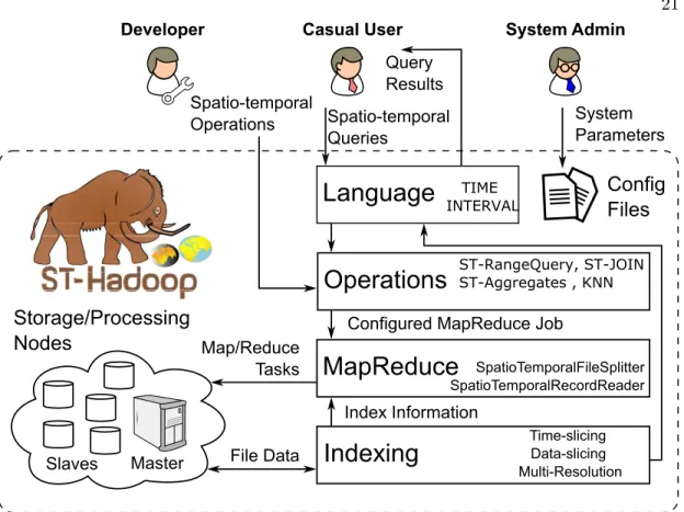
Figure 3.1 gives the high level architecture of our ST-Hadoop system; as the first full-fledged open-source MapReduce framework with a built-in support for spatio-temporal data. ST-Hadoop cluster contains one master node that breaks a map-reduce job into smaller tasks, carried out by slave nodes. Three types of users interact with

ST-Hadoop: (1) Casual users who access ST-Hadoop through its spatio-temporal

language to process their datasets. (2) Developers, who have a deeper understanding

of the system internals and can implement new spatio-temporal operations, and (3) Administrators, who can tune up the system through adjusting system parameters in the configuration files provided with the ST-Hadoop installation. ST-Hadoop adopts

a layered design of four main layers, namely, language, Indexing, MapReduce, and

operations layers, described briefly below:

Language Layer: This layer extends Pigeon language [20] to supports spatio-temporal

data types (i.e., STPoint_,time _and interval_{) and spatio-temporal operations (e.g.,}

overlap_{, and} join_{). The Pigeon Language is a high level language complaint with} OGC standards. Details are given in chapter 8.

Indexing Layer: ST-Hadoop spatiotemporally loads and partitions data across

(33)

21

Indexing

MapReduce

Operations

Master Slaves Map/Reduce Tasks

Configured MapReduce Job Spatio-temporal Queries Query Results Index Information

Storage/Processing

Nodes

Language

Spatio-temporal Operations System Admin Casual User Developer

Config

Files

File Data System Parameters SpatioTemporalFileSplitter SpatioTemporalRecordReader Time-slicing Data-slicing Multi-Resolution ST-RangeQuery, ST-JOIN ST-Aggregates , KNN TIME INTERVAL

Figure 3.1: ST-Hadoop system architecture

computation nodes. In this layer ST-Hadoop scans a random sample obtained from the input dataset, bulk-loads its spatio-temporal index that consists of two-layer indexing

of temporal and then spatial. Finally ST-Hadoop replicates its index into temporal

hierarchy index structure to achieve more eﬃcient performance for processing

spatio-temporal queries. ST-Hadoop introduces two techniques for partitioning temporal

dimension of space and data partitioning namely, Time-slicing and Data-slicing. As for the spatial level of partitioning, ST-Hadoop partitions the spatial dimensions using any of the implemented spatial bull-loading partitioning techniques in ST-Hadoop, such as R-tree, R+-tree, Z-Curve, Grid, Quad-tree, or KD-tree. Details of the index layer are given in chapter 4.

(34)

MapReduce layer to enables ST-Hadoop to exploits its spatio-temporal indexes and

realizes spatio-temporal predicates. In particular, SpatioTemporalFileSplitter and

SpatioTemporalRecordReader, which allows to access the two-level of spatio-temporal indexes in ST-Hadoop and reads spatio-temporal within partitions, respectively. We are not going to discuss this layer any further, mainly because few changes made to inject time awareness in this layer. The implementation of MapReduce layer was already discussed in great details [14].

Operations Layer: This layer encapsulates the implementation of three common spatio-temporal operations, namely, spatio-temporal range, nearest neighbor, and join

queries. More operations can be added to this layer by ST-Hadoop developers. Details

of the operations layer are discussed in chapter 5.

The goal of this thesis is to describe how Hadoop as big distributed Map-Reduce systems can be modified in its internal components to support spatio-temporal data and applications. In a nutshell, ST-Hadoop Cluster contains one master node and several worker nodes. The Master node in ST-Hadoop triggers and manages the spatio-temporal operations. Meanwhile, the worker nodes carry the computations as map-reduce tasks. Through this document, we will describe the full stack of ST-Hadoop starting from storage, indexing, operations, and language. In our architecture design, we allow experts users and system administrators to tune ST-Hadoop configuration files, to guide how spatio-temporal data partition, along with other basic cluster configurations. We envision the layered design of ST-Hadoop will act as a research engine for domain experts and research to extends its capability and builds applications on the top-of ST-Hadoop.

(35)

Chapter 4

Spatio-temporal Indexing in

MapReduce Layer

Input files in Hadoop Distributed File System (HDFS) are organized as a heap structure, where the input is partitioned into chunks, each of size 64MB. Given a file, the first 64MB is loaded to one partition, then the second 64MB is loaded in a second partition, and so on. While that was acceptable for typical Hadoop applications (e.g., analysis tasks), it will not support spatio-temporal applications where there is always a need to filter input data with spatial and temporal predicates. Meanwhile, spatially indexed HDFSs, as in SpatialHadoop [14] and ScalaGiST [32], are geared towards queries with spatial predicates only. This means that a temporal query to these systems will need to scan the whole dataset. Also, a spatio-temporal query with a small temporal predicate may end up scanning large amounts of data. For example, consider an input file that includes all social media contents in the whole world for the last five years or so. A query that asks about contents in the USA in a certain hour may end up in scanning all the five years contents of the USA to find out the answer.

ST-Hadoop HDFS organizes input files as spatio-temporal partitions that satisfy one main goal of supporting spatio-temporal queries. ST-Hadoop imposes temporal slicing, where input files are spatiotemporally loaded into intervals of a specific time granularity, e.g., days, weeks, or months. Each granularity is represented as a level in ST-Hadoop index. Data records in each level are spatiotemporally partitioned, such

(36)

(b) ST-Hadoop Daily Level day 1

(a) SpatialHadoop

All data (c) ST-Hadoop Monthly Level month 1 Spatio-temporal query day 365 _{month 12}

Figure 4.1: HDFSs in ST-Hadoop VS SpatialHadoop

that the boundary of a partition is defined by a spatial region and time interval. Figures 4.1(a) and 4.1(b) show the HDFS organization in SpatialHadoop and

ST-Hadoop frameworks, respectively. Rectangular shapes represent boundaries of the

HDFS partitions within their framework, where each partition maintains a 64MB of nearby objects. The dotted square is an example of a spatio-temporal range query. For simplicity, let’s consider a one year of spatio-temporal records loaded to both frame-works. As shown in Figure 4.1(a), SpatialHadoop is unaware of the temporal locality of the data, and thus, all records will be loaded once and partitioned according to their ex-istence in the space. Meanwhile in Figure 4.1(b), ST-Hadoop loads and partitions data records for each day of the year individually, such that each partition maintains a 64MB of objects that are close to each other in both space and time. Note that HDFS parti-tions in both frameworks vary in their boundaries, mainly because spatial and temporal locality of objects are not the same over time. Let’s assume the spatio-temporal query in the dotted square ”find objects in a certain spatial region during a specific month” in Figures 4.1(a), and 4.1(b). SpatialHadoop needs to access all partitions overlapped with query region, and hence SpatialHadoop is required to scan one year of records to get the final answer. In the meantime, ST-Hadoop reports the query answer by accessing

(37)

25 few partitions from its daily level without the need to scan a huge number of records.

4.1

Concept of Hierarchy

ST-Hadoop imposes a replication of data to support spatio-temporal queries with diﬀ

er-ent granularities. The data replication is reasonable as the storage in ST-Hadoop cluster

is inexpensive, and thus, sacrificing storage to gain more eﬃcient performance is not

a drawback. Updates are not a problem with replication, mainly because ST-Hadoop extends MapReduce framework that is essentially designed for batch processing, thereby ST-Hadoop utilizes incremental batch accommodation for new updates.

The key idea behind the performance gain of ST-Hadoop is its ability to load the data in Hadoop Distributed File System (HDFS) in a way that mimics spatio-temporal index structures. To support all spatio-temporal operations including more

sophisti-cated queries over time, ST-Hadoop replicates spatio-temporal data into a Temporal

Hierarchy Index. Figures 4.1(b) and 4.1(c) depict two levels of days and months in

ST-Hadoop index structure. The same data is replicated on both levels, but with diﬀerent

spatio-temporal granularities. For example, a spatio-temporal query asks for objects in one month could be reported from any level in ST-Hadoop index. However, rather than hitting 30 days’ partitions from the daily-level, it will be much faster to access less number of partitions by obtaining the answer from one month in the monthly-level.

A system parameter can be tuned by ST-Hadoop administrator to choose the number

of levels in theTemporal Hierarchy index. By default, ST-Hadoop set its index structure

to four levels of days, weeks, months and years granularities. However, ST-Hadoop users can easily change the granularity of any level. For example, the following code loads taxi

trajectory dataset from ”NYC” file using one-hour granularity, Where the Level and

Granularityare two parameters that indicate which level and the desired granularity, respectively.

trajectory = LOAD ’NYC’ as

(id:int, STPoint(loc:point, time:timestamp)) Level:1 Granularity:1-hour;

(38)

4.2

Index Construction

Figure 4.2 illustrates the indexing construction in ST-Hadoop, which involves two scan-ning processes. The first process starts by scanscan-ning input files to get a random sample, and this is essential because the size of input files is beyond memory capacity, and thus, Hadoop obtains a set of records to a sample that can fit in memory. Next,

ST-Hadoop processes the sample n times, where n is the number of levels in ST-Hadoop

index structure. The temporal slicing in each level splits the sample into m number

of slice (e.g., slice1.m). ST-Hadoop finds the spatio-temporal boundaries by applying

a spatial indexing on each temporal slice individually. As a result, outputs from tem-poral slicing and spatial indexing collectively represent the spatio-temtem-poral boundaries of ST-Hadoop index structure. These boundaries will be stored as meta-data on the master node to guide the next process. The second scanning process physically assigns data records in the input files with its overlapping spatio-temporal boundaries. Note

that each record in the dataset will be assigned n times, according to the number of

levels.

ST-Hadoop index consists of two-layer indexing of a temporal and spatial. The con-ceptual visualization of the index is shown in the right of Figure 4.2, where lines signify how the temporal index divided the sample into a set of disjoint time intervals, and tri-angles symbolize the spatial indexing. This two-layer indexing is replicated in all levels,

where in each level the sample is partitioned using diﬀerent granularity. ST-Hadoop

trade-oﬀstorage to achieve more eﬃcient performance through its index replication. In

general, the index creation of a single level in the Temporal Hierarchygoes through four

consecutive phases, namely sampling, temporal slicing, spatial indexing, and physical writing.

4.2.1 Phase I Sampling

The objective of this phase is to approximate the spatial distribution of objects and how that distribution evolves over time, to ensure the quality of indexing; and thus, enhance the query performance. This phase is necessary, mainly because the input files

are too large to fit in memory. ST-Hadoop employs a map-reduce job to eﬃciently read

(39)

27 Samp ling Bulk-loadin g

Scan I

Scan II

sample T ime S lice Level 1

Slice 1.1 Slice 1.2 Slice 1.m

Spatial Indexing Spatial Indexing Spatial Indexing Spatio-tempor al Bound aries Level 1 Physical W riting Level 1 Physical W riting Level n T ime S lice Level n Spatial Indexing Spatial Indexing Spatial Indexing Spatio-tempor al Bound aries Level n Level 1 Level n

Slice n.1 Slice n.2 Slice n.m Fi

gu re 4. 2: In d ex in g in S T -H ad o op

(40)

data structure of a length (L), that is an equal to the number of HDFS blocks, which

can be directly calculated from the equation L = (Z/B), where Z is the total size of

input files, and B is the HDFS block capacity (e.g., 64MB). The size of the random

sample is set to a default ratio of 1% of input files, with a maximum size that fits in the memory of the master node. This simple data structure represented as a collection of elements; each element consist of a time instance and a space sampling that describe the time interval and the spatial distribution of spatio-temporal objects, respectively. Once the sample is scanned, we sort the sample elements in chronological order to their time instance, and thus the sample approximates the spatio-temporal distribution of input files.

4.2.2 Phase II Temporal Slicing

In this phase ST-Hadoop determines the temporal boundaries by slicing the in-memory

sample into multiple time intervals, to eﬃciently support a fast random access to a

se-quence of objects bounded by the same time interval. ST-Hadoop employs two temporal slicing techniques, where each manipulates the sample according to specific slicing

char-acteristics: (1) Time-partition, slices the sample into multiple splits that are uniformly

on their time intervals, and (2) Data-partition where the sample is sliced to the degree

that all sub-splits are uniformly in their data size. The output of this phase finds the temporal boundary of each split, that collectively cover the whole time domain.

The rational reason behind ST-Hadoop two temporal slicing techniques is that for some spatio-temporal archive the data spans a long time-interval such as decades, but their size is moderated compared to other archives that are daily collect terabytes or petabytes of spatio-temporal records. ST-Hadoop proposed the two techniques to slice the time dimension of input files based on either time-partition or data-partition,

to improve the indexing quality, and thus gain eﬃcient query performance. The

time-partition slicing technique serves best in a situation where data records are uniformly distributed in time. Meanwhile, data-partition slicing best suited with data that are sparse in their time dimension.

(41)

29

HDFS

Figure 4.3: Data-Slice

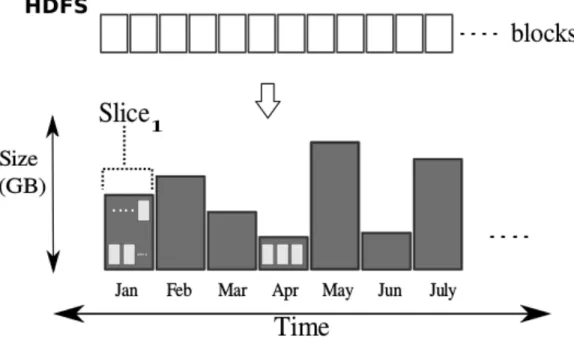
the degree that all sub-splits are equally in their size. Figure 4.3 depicts the

key concept of this slicing technique, such that a slice1 and slicen are equally

in size, while they diﬀer in their interval coverage. In particular, the temporal

boundary of slice1 spans more time interval thanslicen. For example, consider

128MB as the size of HDFS block and input files of 1 TB. Typically, the data will be loaded into 8 thousand blocks. To load these blocks into ten equally balanced slices, ST-Hadoop first reads a sample, then sort the sample, and apply

Data-partitiontechnique that slices data into multiple splits. Each split contains around 800 blocks, which hold roughly a 100 GB of spatio-temporal records. There might be a small variance in size between slices, which is expectable. Similarly, another level in ST-Hadoop temporal hierarchy index could loads the 1 TB into 20 equally balanced slices, where each slice contains around 400 HDFS blocks. ST-Hadoop users are allowed to specify the granularity of data slicing by tuning

α parameter. By default four ratios of α is set to 1%, 10%, 25%, and 50% that

(42)

Size

(GB)

1

....

Figure 4.4: Time-Slice

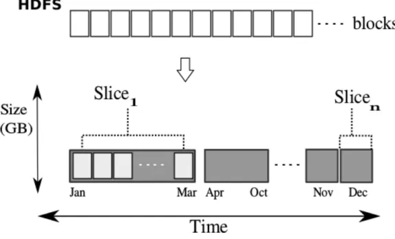
∗ Time-partition Slicing. The ultimate goal of this approach is to slices the input files into multiple HDFS chunks with a specified interval. Figure 4.4 shows the general idea, where ST-Hadoop splits the input files into an interval of one-month granularity. While the time interval of the slices is fixed, the size of data within slices might vary. For example, as shown in Figure 4.4 Jan slice has more HDFS blocks than April.

ST-Hadoop users are allowed to specify the granularity of this slicing technique, which specified the time boundaries of all splits. By default, ST-Hadoop finer gran-ularity level is set to one-day. Since the grangran-ularity of the slicing is known, then a straightforward solution is to find the minimum and maximum time instance of the sample, and then based on the intervals between the both times ST-Hadoop hashes el-ements in the sample to the desired granularity. The number of slices generated by the time-partition technique will highly depend on the intervals between the minimum and the maximum times obtained from the sample. By default, ST-Hadoop set its index structure to four levels of days, weeks, months and years granularities.

(43)

31 4.2.3 Phase III Spatial Indexing

This phase ST-Hadoop determines the spatial boundaries of the data records within each temporal slice. ST-Hadoop spatially index each temporal slice independently; such decision handles a case where there is a significant disparity in the spatial distribution between slices, and also to preserve the spatial locality of data records. Using the same

sample from the previous phase, ST-Hadoop takes the advantages of applying diﬀerent

types of spatial bulk loading techniques in HDFS that are already implemented in SpatialHadoop such as Grid, R-tree, Quad-tree, and Kd-tree. The output of this phase is the spatio-temporal boundaries of each temporal slice. These boundaries stored as a data in a file on the master node of ST-Hadoop cluster. Each entry in the

meta-data represents a partition, such as< id, M BR, interval, level >. Whereidis a unique

identifier number of a partition on the HDFS, M BR is the spatial minimum boundary

rectangle, interval is the time boundary, and the level is the number that indicates

which level in ST-Hadoop temporal hierarchy index. 4.2.4 Phase IV Physical Writing

Given the spatio-temporal boundaries that represent all HDFS partitions, we initiate a map-reduce job that scans through the input files and physically partitions HDFS block, by assign data records to overlapping partitions according to the spatio-temporal boundaries in the meta-data stored on the master node of ST-Hadoop cluster. For each

record r assigned to a partition p, the map function writes an intermediate pair ⟨p, r⟩

Such pairs are then grouped byp and sent to the reduce function to write the physical

partition to the HDFS. Note that for a record r will be assigned n times, depends on

the number of levels in ST-Hadoop index.

4.3

Index Maintenance

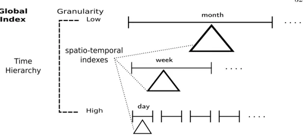
This index structure can be described as a temporal hierarchy for spatio-temporal indices as shown in Figure 4.5. ST-Hadoop merges a set of temporal slices from the lower most layer to create a slice with a larger time interval. For simplicity let’s assume the lowermost layer was sliced into days, then ST-Hadoop combines a set days to create a

(44)

Time Hierarchy spatio-temporal indexes t1 Low High Granularity Global Index day week month

Figure 4.5: Temporal Hierarchy Index

week-slice in the layer above. Likewise, ST-Hadoop reads a sample from the merged set to bulk load its spatio-temporal index. Note that this step is necessary as the size and the distribution of objects vary from a lower (i.e., day) to the above layer (i.e., week). For each layer in the hierarchical index, ST-Hadoop iterates two-level bulk

loading techniques of a temporal and then spatial, with diﬀerent time granularity. A

system parameter can be tuned by ST-Hadoop administrator to choose the number of

layers and their granularity. By default, ST-Hadoop set its temporal hierarchy index to

four layers with a resolution of days, weeks, months and years, respectively. Similarly,

the granularity of the four layers in Data-based slicing will have diﬀerent slicing ratios

(α), such as 1%, 10%, 25%, and 50%.

ST-Hadoop in a regular base such as every day maintains its Temporal Hierarchy

Index, to reflects updates on the index with the incoming data. First, it creates a new two-level indexing in the lowest layer using one MapReduce job to index spatio-temporal records similar to the same granularity of that layer. Then check if the newly created index will help to create an index in the above layer, if not then it will be carried out for a next maintenance call. During the maintenance, if there is any indices contribute to the above layer, then data of these indices will be merged, and a new two-level indexing will be created with a bigger granularity.

(45)

33 Table 4.1: Twitter Datasets

Twitter Data Size Num-Records Time window

Large 10TB >1 Billion > 3 years

Average-Large 6.7TB 692 Million 1 years

Medium-Large 3TB 152 Million 9 months

Moderate-Large (1TB) 115 Million 3 months

4.4

Experiments

This section provides an extensive experimental performance study of ST-Hadoop com-pared to SpatialHadoop and Hadoop. We decided to compare with this two frameworks and not other spatio-temporal DBMSs for two reasons. First, as our contributions are

all about spatio-temporal data support in Hadoop. Second, the diﬀerent architectures

of spatio-temporal DBMSs have great influence on their respective performance, which is out of the scope of this paper. Interested readers can refer to a previous study [77]

which has been established to compare diﬀerent large-scale data analysis architectures.

In other words, ST-Hadoop is targeted for Hadoop users who would like to process large-scale spatio-temporal data but are not satisfied with its performance. The experiments

are designed to show the eﬀect of ST-Hadoop indexing and the overhead imposed by its

new features compared to SpatialHadoop. However, ST-Hadoop achieves two orders of magnitude improvement over SpatialHadoop and Hadoop.

4.4.1 Experimental Settings

Cluster Setup. All experiments are conducted on a dedicated internal cluster of 24 nodes. Each has 64GB memory, 2TB storage, and Intel(R) Xeon(R) CPU 3GHz of 8 core processor. We use Hadoop 2.7.2 running on Java 1.7 and Ubuntu 14.04.5 LTS. Table 4.2 summarizes the configuration parameters used in our experiments. Default parameters (in parentheses) are used unless mentioned.

Datasets. To test the performance of ST-Hadoop we use the Twitter archived dataset [2]. The dataset collected using the public Twitter API for more than three years, which contains over 1 Billion spatio-temporal records with a total size of 10TB.

(46)

Table 4.2: ST-Hadoop Experiments Parameters

Parameter Values (default)

HDFS block capacity (B) 32, 64, (128), 256 MB

Cluster size (N) 5, 10, 15, 20, (23)

Selection ratio (ρ) (0.01), 0.02, 0.05, 0.1, 0.2, 0.5, 1.0

Data-partition slicing ratio(α) 0.01, 0.02, 0.025, 0.05, (0.1), 1

Time-partition slicing granularity(σ) (days), weeks, months, years

Spatio-temporal proximity (α) 0,0.2, (0.5), 0.6, 0.8, 1.0

and sizes, respectively as shown in Table 4.1. The default size used is 1TB which is big enough for our extensive experiments unless mentioned.

4.4.2 Index Construction

Figure 4.6(a) gives the total time for building the spatio-temporal index in ST-Hadoop. This is a one time job done for input files. In general, the figure shows excellent scal-ability of the index creation algorithm, where it builds its index using data-partition slicing for a 1TB file with more than 115 Million records in less than 15 minutes. The data-partition technique turns out to be the fastest as it contains fewer slices than time-partition. Meanwhile, the time-partition technique takes more time, mainly be-cause the number of partit