Trapped modes in a waveguide with a long obstacle

(1)

Additional services for Journal of Fluid Mechanics:

Email alerts: Click here Subscriptions: Click here Commercial reprints: Click here Terms of use : Click here

Trapped modes in a waveguide with a long obstacle

N. S. A. KHALLAF, L. PARNOVSKI and D. VASSILIEV

Journal of Fluid Mechanics / Volume 403 / January 2000, pp 251 261 DOI: 10.1017/S0022112099007028, Published online: 08 September 2000

Link to this article: http://journals.cambridge.org/abstract_S0022112099007028

How to cite this article:

N. S. A. KHALLAF, L. PARNOVSKI and D. VASSILIEV (2000). Trapped modes in a waveguide with a long obstacle. Journal of Fluid Mechanics, 403, pp 251261 doi:10.1017/S0022112099007028

Request Permissions : Click here

(2)

c

2000 Cambridge University Press

Trapped modes in a waveguide with

a long obstacle

By N. S. A. K H A L L A F1_†_{, L. P A R N O V S K I}2

AND D. V A S S I L I E V3

1_{University of King Abdulaziz, College of Education, Department of Mathematics, Al-Madinah}

Al-Munawwarah, PO Box 344, Kingdom of Saudi Arabia

2_{School of Mathematical Sciences, University of Sussex, Brighton BN1 9QH, UK} 3_{Department of Mathematical Sciences, University of Bath, Claverton Down,}

Bath BA2 7AY, UK

(Received 7 October 1998 and in revised form 13 September 1999)

Consider an infinite two-dimensional acoustic waveguide containing a long rectan-gular obstacle placed symmetrically with respect to the centreline. We search for trapped modes, i.e. modes of oscillation at particular frequencies which decay down the waveguide. We provide analytic estimates for trapped mode frequencies and prove that the number of trapped modes is asymptotically proportional to the length of the obstacle.

1. Introduction

In this paper we consider an infinite planar waveguide containing an obstacle. We assume that the waveguide is occupied by an acoustic medium and study the free vibrations of this medium. Mathematically the problem is described by the Helmholtz equation for the potential of displacements φ(x, y), subject to Neumann boundary conditions on the sides of the waveguide and on the boundary of the obstacle (hard walls). The same mathematical problem appears in the study of water waves in channels; see, for example, Evans & Linton (1991) and Callan, Linton & Evans (1991).

If for a particular vibration frequency the problem has a non-trivial solution decaying at infinity, we shall say that we have a trapped mode. As pointed out in Evans, Levitin & Vassiliev (1994), Roitberg, Vassiliev & Weidl (1998) and Davies & Parnovski (1998) the existence of trapped modes is usually related to certain symmetries in the problem. In this paper we deal with the most basic type of symmetry, namely when the obstacle is symmetric about the centreline. We restrict ourselves to the study of antisymmetric modes, and search for trapped mode eigenvalues below the first antisymmetric cutoff.

(3)

y

x N

N N

– a a

N

–1

–b b

1

N

Figure 1.Domain ˜Ω.

by other authors, see, for example, Evans & Linton (1991), Evans (1992) and Evans & Linton (1992).

The main result of our paper is that asa→+∞the total number of trapped modes is asymptotically equal to a (see Corollary 3 in §3). Thus, for a long rectangular obstacle the total number of trapped modes is asymptotically determined only by the length of the obstacle. Moreover, we prove (Theorem 5.1) that the same is true for long obstacles of fairly general shape. Numerical results are given in §4.

We were to a large extent motivated by Evans & Linton (1991), Evans (1992) and Evans & Linton (1992). Though the numerical results of these authors do not extend to very long obstacles, they helped us predict the asymptotics. Moreover, for b= 0 our asymptotics can be obtained directly from Evans (1992).

2. Statement of the problem

Let ˜Ω be the unbounded planar domain defined as ˜

Ω={(−∞,∞)×(−1,1)} \ {[−a, a]×[−b, b]}

(see figure 1), wherea >0 and 06b <1. We are interested in finding trapped modes, i.e. eigenvalues of the Neumann Laplacian in ˜Ω. In other words, we are looking for the values ofλfor which there exists a non-trivial square-integrable solution φ(x, y) of the Helmholtz equation

−∆φ=λφ in ˜Ω (2.1)

subject to the boundary conditions ∂φ

∂n∂Ω˜ = 0 (2.2)

(note that the boundary∂Ω˜ is the union of the boundary of the strip and the boundary of the obstacle). The spectral parameter λis related to the vibration frequency ω as λ=ω2_/c2_{, where}_c _{is the speed of sound in the medium.}

(4)

y

x N

D

0

N

– a a

b

1

N N

D

Figure 2.DomainΩ+_.

problem because they are extremely unstable and can be destroyed by an arbitrarily small perturbation.

However, in our special case the situation is simplified because of the symmetry; see Evanset al. (1994), Roitberg et al. (1998) and Davies & Parnovski (1998) for a discussion of the notion of symmetry in this setting. Namely, let us consider functions which are odd in y:

H1:={φ∈L2( ˜Ω)|φ(x,−y) =−φ(x, y)}.

One can easily check that H1 is an invariant subspace of L2( ˜Ω) with respect to the action of −∆. Moreover, the essential spectrum of −∆|H1 is the interval [π2/4,∞). Therefore, the eigenvalues of −∆|H1 lying in [0,π2/4) are stable under small pertur-bations, and one can find such eigenvalues using standard variational methods. The spectral problem for −∆|H1 is equivalent to the spectral problem for the Laplace operator in

Ω+ _:=_{_{(x, y)}_∈_Ω_˜_|_{y >}₀_}

with Neumann boundary conditions on the ‘old’ boundary and Dirichlet boundary conditions on the ‘new’ boundary {(x, y)|y = 0,|x| > a}, see figure 2. Hence, the problem is reduced to finding values of λ for which there is a non-trivial square integrableφ(x, y) satisfying the Helmholtz equation

−∆φ=λφ inΩ+ _(2.3)

subject to the boundary conditions ∂φ

∂yy=1 = 0, (2.4)

∂φ

∂y|x|<a, y=b = 0, (2.5) ∂φ

∂x|x|=a,0<y<b = 0, (2.6)

φ||x|>a, y=0 = 0. (2.7)

All the eigenvalues of (2.3)–(2.7) lying in [0,π2_{/4) can be found using the variational} approach. Put

Q(φ) :=

Z Z

Ω+|∇φ| 2_dx_dy

Z Z

Ω+|φ|

(5)

b N

0

N

a

D N

1

Figure 3.DomainΩ.

λ1 := infQ(φ), (2.9)

where the infimum is taken over functions φ 6≡ 0 satisfying the boundary condition (2.7) (here we do not have to impose the Neumann conditions (2.4)–(2.6) because they are automatically satisfied at the extrema of Q(φ)). Now, if λ1 <π2/4, thenλ1 is the first eigenvalue of (2.3)–(2.7) and the function φ1 on which the infimum is attained is the eigenfunction corresponding to λ1. (It is easy to see that λ1 >0.) Analogously, if λ2 := infφ⊥φ1Q(φ) <π2/4, then λ2 is the second eigenvalue of (2.3)–(2.7) and the function φ2 on which the infimum is attained is the eigenfunction corresponding to λ2. This procedure can be repeated until we getλk+1 =π2/4. Then we will know that in the interval (0,π2_{/4) there are exactly}_k _{eigenvalues of the problem (2.3)–(2.7) and} these eigenvalues areλ1, . . . , λk. However, we still will not be able to say anything about eigenvalues lying in [π2_/4,_∞_{). To find them one should either use a different approach,} or find a new symmetry which will move the continuous spectrum further up.

In our case there is another obvious symmetry – reflection with respect to the y-axis. This symmetry does not change the continuous spectrum, but nevertheless makes computations easier. So let us consider the two subspaces

H±_:=_{_φ_∈_L2_(Ω+₎_|_φ(₋_{x, y) =}_±_{φ(x, y)}_}_.

These subspaces are invariant under the action of−∆. Therefore, the spectrum of the problem (2.3)–(2.7) is the union of the spectra of the restrictions of (2.3)–(2.7) toH+ andH−_{. Moreover, the spectrum of (2.3)–(2.7) restricted to}_H+₍_H−_{) coincides with}

the spectrum of−∆ considered in

Ω :={(x, y)∈Ω+_|_{x >}₀_}

with unchanged boundary conditions on the ‘old’ boundary and Neumann (Dirichlet) boundary conditions on the ‘new’ boundary {(x, y)|x= 0, b < y <1}, see figure 3.

The continuous spectra of both these problems are still [π2_/4,_∞_{), but using the} variational approach described above one can find the eigenvalues of these problems below π2_{/4. Let us call such eigenvalues} _λN

1, . . . , λNkN and λD1, . . . , λDkD respectively, so that there are kN (kD) eigenvalues of these problems belowπ2/4.

3. Explicit estimates for eigenvalues

The aim of this section is to prove the following. Theorem 3.1. Let λN

j , λDj ∈ (0,π2/4) be the eigenvalues defined above. Then the following inequalities hold for all j:

π2

a2(j−1)26λNj 6 π 2 a2 j−12

2

(6)

and

π2 a2 j− 12

2₆_λ_D j 6 π

2

a2j2. (3.2)

Moreover, each interval (3.1), (3.2) with right endpoint < π2_/4 _{contains one and only}

one eigenvalue.

Before giving the proof of this theorem let us state its immediate implications. We define the counting functionNN_{(λ) (N}D_{(λ)) to be the number of eigenvalues}_λN

j (λD

j) which are less thanλ. We also defineNtotal:=NN(π2/4)+ND(π2/4) =kN+kD. In other words,Ntotal _{is the total number of trapped modes antisymmetric with respect} to the centreline with frequencies below the cutoff frequency (the frequency above which one gets propagating antisymmetric modes).

In what follows [z] stands for the greatest integer strictly less thanz; that is, [z] is the integer part of z if z is non-integer, and [z] =z−1 if z is integer. Theorem 3.1 implies

Corollary 1. Let λ∈(0,π2_/4]_{. Then}

h_a

πλ1/2

i

6ND_(λ)₆_NN_(λ)₆ha

πλ1/2

i

+ 1. (3.3)

Corollary 2. Let λ ∈ (0,π2_/4] _{be fixed. Then the following asymptotic formulae}

hold as a→+∞:

NN_(λ)_∼ a

πλ1/2, ND(λ)∼

a

πλ1/2. (3.4)

Corollary 3. The following asymptotic formula for the total number of trapped modes holds as a→+∞:

Ntotal_∼_a. _(3.5)

Proof of Theorem 3.1. Let us prove formula (3.1) (formula (3.2) is proved similarly). Throughout the proof we will be dropping the superscript N referring to the type of boundary condition on the y-axis. In particular, we shall write N(λ) = NN_{(λ). The} number λwill be assumed to satisfy 0< λ <π2_/4.

The main idea is to use Dirichlet–Neumann bracketing along the line x=a. Let us cut Ω into two domains: A:={(x, y)∈ Ω|x < a}and B := {(x, y) ∈Ω|x > a}. Denote by λA,N

j (λA,Dj ) the eigenvalues of −∆ acting in the domain A with Neumann (Dirichlet) boundary conditions on the ‘new’ boundary{(x, y)|x=a, b < y <1}and the same boundary conditions on the ‘old’ boundary as before; of course, the latter means having Neumann boundary conditions on the top, bottom, and left-hand sides ofA. In the same way we defineλB,N_j andλB,D_j . LetNN

A(λ) be the number of eigenvalues λA,N

j which are less than λ; similarly we define the three other counting functions. Let us emphasize that now the letters N and D stand for boundary conditions on the intervalx=a, b < y <1, and not on they-axis!

The essential spectrum of all the operators involved is either empty (−∆ acting on A), or [π2_/4,_∞_{) (}₋_{∆ acting on}_B _or_{Ω). We have assumed that}_{λ <}_π2_{/4, therefore the} variational principle implies the following formula, known as the Dirichlet–Neumann bracketing (see e.g. Courant & Hilbert, Theorem VI.2.5):

ND

(7)

b

0

a

1

N

c D

D

Figure 4.Truncated domainΩ.

Using separation of variables one can easily compute the eigenvalues onA: say, if we have Dirichlet conditions on the right-hand side, then

n

λA,D j

o∞

j=1 =

π2 a2 n− 12

₂

+ π2

(1−b)2(m−1)2

∞

n,m=1

. (3.7)

In a similar way

n

λA,N j

o∞

j=1 =

π2

a2(n−1)2+

π2

(1−b)2(m−1)2

∞

n,m=1

. (3.8)

Note that the values of the expressions in the right-hand sides of (3.7)–(3.8) corresponding tom >1 are greater thanπ2_{/4, therefore, when dealing with eigenvalues} belowπ2_{/4, we may assume that}_m_{= 1. Let us now look at the sets}_{_λB,N

j } ∩[0,π2/4) and {λB,D_j } ∩[0,π2_{/4). Using separation of variables one can easily show that the first} of these two sets is empty. Indeed, the spectrum of−∆ onB with Neumann boundary conditions on the top and left-hand sides and Dirichlet boundary condition on the bottom side is the interval [π2_/4,_∞_{). Let us now prove that} _{_λB,D

j } ∩[0,π2/4) = ∅. Suppose that λB,D

1 <π2/4. Then the variational principle impliesλB,N1 <π2/4, and we have just seen that this is not the case. Therefore, for λ <π2_{/4 we have}

ND

A(λ)6N(λ)6NAN(λ). (3.9)

Formulae (3.7)–(3.9) imply (3.1).

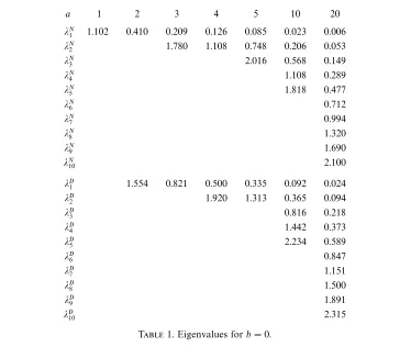
4. Numerical results

In this section we provide some numerical results for the eigenvalues λN

j and λDj introduced at the end of§2.

Computations were done using the variational method. Namely, we considered the Rayleigh quotientQ(φ) on Ω (see (2.8)) and, minimizing it, successively determined the eigenvalues and eigenfunctions. Applying this procedure we imposed Dirichlet boundary conditions on the appropriate parts of∂Ω, but did not impose Neumann ones because they are automatically satisfied at the extrema ofQ(φ). The discretization ofQ(φ) was carried out over a square mesh with mesh sizeh= 1/20. We truncated our domainΩto a finite one by imposing a Dirichlet boundary condition atx=c= 40, see figure 4. (Our numerical calculations showed that the dependence of the eigenvalues on the choice ofc is hardly noticeable for c> 40.) The actual minimization of the (discretised)Q(φ) was performed by the gradient method. As the first approximation for thenth eigenfunction we took

φ(x, y) =

sin (n/a)πx for x6a

(8)

a 1 2 3 4 5 10 20 λN

1 1.102 0.410 0.209 0.126 0.085 0.023 0.006

λN

2 1.780 1.108 0.748 0.206 0.053

λN

3 2.016 0.568 0.149

λN

4 1.108 0.289

λN

5 1.818 0.477

λN

6 0.712

λN

7 0.994

λN

8 1.320

λN

9 1.690

λN

10 2.100

λD

1 1.554 0.821 0.500 0.335 0.092 0.024

λD

2 1.920 1.313 0.365 0.094

λD

3 0.816 0.218

λD

4 1.442 0.373

λD

5 2.234 0.589

λD

6 0.847

λD

7 1.151

λD

8 1.500

λD

9 1.891

λD

10 2.315

Table 1.Eigenvalues forb= 0.

in the case of the Dirichlet boundary condition on they-axis, and

φ(x, y) =

cos ((n− 1

2)/a)πx forx6a

0 forx>a (4.2)

in the case of the Neumann one. It turns out that the graphs of the actual eigen-functions (which we omit for the sake of brevity) are remarkably close to (4.1) and (4.2).

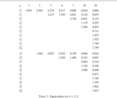
Our main numerical results are presented in tables 1 and 2. Of course, forathat are not too large these results agree with those of Evans & Linton (1991). The accuracy of our numerical results is determined by two main factors: the choice of truncation distance c and mesh size h. Elementary analysis involving separation of variables shows that imposing an artificial boundary condition at x=cintroduces an error of the order of e−√π2_/₄₋_λ_j(_c₋_a₎

which is negligible for our values ofa, candλj. Predicting the error arising from the choice of mesh size is more complicated, but our numerical experiments with the refinement fromh= 1/10 toh= 1/20 indicate that the relative error in the determination of theλj is not greater than 1%.

(9)

a 1 2 3 4 5 10 20 λN

1 1.494 0.484 0.234 0.137 0.089 0.024 0.006

λN

2 2.237 1.295 0.841 0.216 0.055

λN

3 2.330 0.601 0.152

λN

4 1.178 0.297

λN

5 1.946 0.493

λN

6 0.731

λN

7 1.023

λN

8 1.362

λN

9 1.746

λN

10 2.186

λD

1 1.888 0.925 0.545 0.359 0.094 0.024

λD

2 2.299 1.496 0.385 0.097

λD

3 0.865 0.219

λD

4 1.538 0.388

λD

5 2.404 0.606

λD

6 0.872

λD

7 1.186

λD

8 1.550

λD

9 1.962

λD

10 2.423

Table 2.Eigenvalues forb= 1/2.

y

x a – a

Figure 5.Obstacle of fairly general shape.

the boundary with the Neumann condition. It is known that in such a situation the eigenvalues are not, in general, domain monotone.

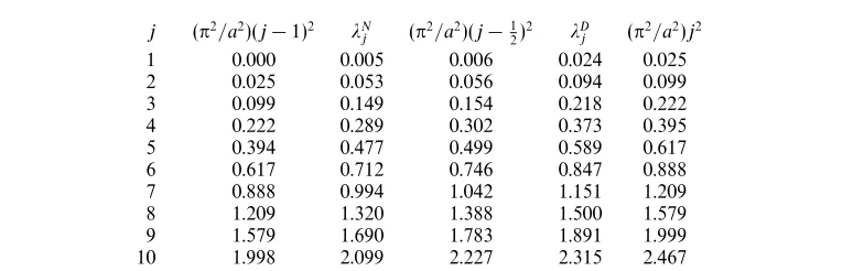
Table 3 provides a numerical illustration of Theorem 3.1. This table indicates that our upper estimate is in most cases closer to the actual eigenvalue than the lower one.

5. Long obstacles of general shape

(10)

j (π2_/a2₎₍_j₋₁₎2 _λN

j (π2/a2)(j−12)2 λDj (π2/a2)j2

1 0.000 0.005 0.006 0.024 0.025

2 0.025 0.053 0.056 0.094 0.099

3 0.099 0.149 0.154 0.218 0.222

4 0.222 0.289 0.302 0.373 0.395

5 0.394 0.477 0.499 0.589 0.617

6 0.617 0.712 0.746 0.847 0.888

7 0.888 0.994 1.042 1.151 1.209

8 1.209 1.320 1.388 1.500 1.579

9 1.579 1.690 1.783 1.891 1.999

10 1.998 2.099 2.227 2.315 2.467

Table 3.Numerical illustration of Theorem 3.1 (a= 20,b= 0).

Leta >0 be a real parameter. Put

Oa:= m

[

i=1

{(x, y)|x∈ [aXi−1, aXi], 06y6fi(x/a)}

(so thatOais an obstacle of length 2a). Let us consider the problem (2.1) in the domain Ω+

a := (−∞,∞)×(0,1)\ Oa with Neumann boundary conditions on {y = 1} ∪∂Oa and Dirichlet boundary conditions on {|x|> a, y = 0}. Figure 5 shows an example of such an obstacle. We denote by N(λ) the number of eigenvalues of this problem belowλ, and put Ntotal_:=_N₍_π2_{/4). The aim of this section is to prove the following} theorem which generalizes Corollaries 2 and 3 from §3.

Theorem 5.1. Letλ∈(0,π2_/4] _{be fixed. Then}

N(λ)∼ 2a

πλ1/2 (5.1)

as a→+∞. In particular,

Ntotal_∼_a. _(5.2)

Proof. In order to prove (5.1) we have to show that

N(λ)> 2a

√

λ

π −o(a) (5.3)

and

N(λ)< 2a

√

λ

π +o(a). (5.4)

We shall, as before, prove these estimates using Dirichlet–Neumann bracketing. We first prove (5.3). Let ε >0 be a small number. Put

ni=ni(ε, a) :=

"

a(Xi−Xi−1) √

λ−ε

π

#

, i= 1, . . . , m, (5.5)

xi,j=xi,j(ε, a) :=a

Xi−1+ j(Xi−_nXi−1) i

(11)

and impose additional Dirichlet conditions on the vertical intervals

{(x, y)|x=xi,j, fi(x/a)< y <1}, i= 1, . . . , m, j= 0,1, . . . , ni. (5.6) The variational principle implies that the spectrum of this new problem (i.e. the problem (2.1) with Neumann boundary conditions on {y = 1} ∪∂O and Dirichlet boundary conditions on{|x|> a, y= 0}and on (5.6)) is higher than that of the initial problem. In other words, N(λ) can be estimated from below by the corresponding counting function of the new problem. The latter is, in turn, not less than

m

X

i=1 ni

X

j=1 Ni,j(λ).

HereNi,j(λ) is the number of eigenvalues of the Laplacian on the ‘almost rectangle’ Ωi,j :={(x, y)|xi,j−1< x < xi,j, fi(x/a)< y <1}

with Neumann boundary conditions on the horizontal sides y = 1 and y = fi(x/a) and Dirichlet boundary conditions on the vertical sides x=xi,j−1 andx=xi,j. When a → ∞ all ‘almost rectangles’ Ωij converge to proper rectangles of width π/√λ−ε, and the convergence is uniform in i, j. We now want to show that

Ni,j(λ)>1 (5.7)

for large enough a uniformly over i, j. In fact, it is easy to show (see, for example, Stollmann 1995) that the spectra of the Ωij converge to the spectra of proper rectangles (with corresponding boundary conditions) uniformly in i, j. Since the bottom eigenvalue of the proper rectangles is λ − ε, this would imply (5.7). To make the proof self-contained, we will also prove (5.7) directly. Indeed, consider the following test function φij:Ωij→R:

φij(x, y) = sin

π(x−xi,j−1) xi,j−xi,j−1

.

Whena→ ∞, both expressions

Z Z

Ωij

|∇φij|2dxdy

and _{Z Z}

Ωij

|φij|2_dx_dy

converge to the corresponding integrals over the limiting rectangles uniformly over i, j. This means that their ratio

Q(φij) =

Z Z

Ωij

|∇φij|2_dx_dy

Z Z

Ωij

|φij|2_dx_dy

(12)

the inequality (5.7) is indeed fulfilled. Therefore,

N(λ)>

m

X

i=1 ni

X

j=1

Ni,j(λ)>

m

X

i=1 ni

X

j=1 1 =

m

X

i=1

ni> 2a

√

λ−ε

π −m=

2a√λ

π −m+O(εa).

Since ε >0 is arbitrary, this implies (5.3).

The proof of (5.4) is analogous, the only difference being that we replace (5.5) by

ni=ni(ε, a) :=

a(Xi−Xi−1)√λ+ε

π

and impose Neumann conditions on the vertical intervals (5.6).

REFERENCES

Callan, M., Linton, C. M. & Evans, D. V.1991 Trapped modes in two-dimensional waveguides.

J. Fluid Mech.229, 51–64.

Courant, R. & Hilbert, D.1989Methods of Mathematical Physics I.Wiley.

Davies, E. B. & Parnovski, L.1998 Trapped modes in acoustic waveguides.Q. J. Mech. Appl. Maths 51, 477–492.

Evans, D. V.1992 Trapped acoustic modes.IMA J. Appl. Maths49, 45–60.

Evans, D. V., Levitin, M. & Vassiliev, D.1994 Existence theorems for trapped modes.J. Fluid. Mech.261, 21–31.

Evans, D. V. & Linton, C. M.1991 Trapped modes in open channels.J. Fluid. Mech.225, 153–175. Evans, D. V. & Linton, C. M.1992 Acoustic resonance in ducts.J. Sound Vib.173, 85–94. Roitberg, I., Vassiliev, D. & Weidl, T.1998 Edge resonance in an elastic semi-strip.Q. J. Mech.

Appl. Maths51, 1–13.