Evaluation of candidate geomagnetic field models for the 10th generation of
IGRF
Stefan Maus1, Susan Macmillan2, Frank Lowes3, and Tatjana Bondar4
1National Geophysical Data Center, Boulder, 80305, U.S.A. 2British Geological Survey, Edinburgh, EH9 3LA, U.K.
3Physics Department, University of Newcastle, Newcastle Upon Tyne, NE1 7RU, U.K. 4IZMIRAN, Moscow 142190, Russia
(Received February 18, 2005; Accepted June 10, 2005)
The recent satellite magnetic missions, combined with high quality ground observatory measurements, have provided excellent data for main field modelling. Four different groups submitted seven main-field and eight secular-variation candidate models for IGRF-10. These candidate models were evaluated using several different strategies. Comparing models with independent data was found to be difficult. Valuable information was gained by mapping model differences, computing root mean square differences between all pairs of models and between models and the common mean, and by studying power spectra and azimuthal distributions of coefficient power. The resulting adopted IGRF main-field model for 2005.0, an average of three selected candidate models, is estimated to have a formal root mean square error over the Earth’s surface of only 5 nT, though it is likely that the actual error is somewhat larger than this. Due to the inherent uncertainty in secular variation forecasts, the corresponding error of the adopted secular-variation model for 2005.0–2010.0, an average of four selected candidate models, is estimated at 20 nT/a.
Key words:Geomagnetism, field modeling, reference field, secular variation.
1.
Introduction
For the 10th generation IGRF a total of seven main-field (MF) candidate models for 2005.0, and eight linear secular-variation (SV) candidate models for 2005.0–2010.0, were submitted for evaluation to a Task Force set up by IAGA Working Group V-MOD. The candidate models were sub-mitted by Danish Space Research Institute in collabora-tion with NASA and Newcastle University (DSRI-NASA-Newcastle model, group A), by US National Geophysi-cal Data Center and GeoForschungsZentrum (NGDC-GFZ model, group B), British Geological Survey (BGS model, group C) and Institute of Terrestrial Magnetism, Ionosphere and Radio Wave Propagation (IZMIRAN model, group D). Comparisons of candidate models with actual measure-ments are difficult due to the limited availability of inde-pendent data. Also, single, localized measurements con-tain contributions from other sources of the magnetic field, in particular the crust, ionosphere and magnetosphere and time-varying fields induced in the Earth. Additionally, the models are predictions of the field for the upcoming epoch, for which measurements are not yet available. Attempts to evaluate the IGRF-10 candidate models using independent data remained inconclusive.
After a brief description of the candidate models, this paper shows how the MF and SV models were evaluated separately using several different strategies. We found that
Copyright cThe Society of Geomagnetism and Earth, Planetary and Space
Sci-ences (SGEPSS); The Seismological Society of Japan; The Volcanological Society of Japan; The Geodetic Society of Japan; The Japanese Society for Planetary Sci-ences; TERRAPUB.
good insight was gained by comparing the models at the surface of the Earth as difference maps and tables of root mean square differences. The analysis of power spectra was a further useful tool, in particular for studying differences at higher spherical harmonic degrees.
For the secular variation an important issue was whether the optimum estimate of the change of the field from 2005.0 to 2010.0 by a linear SV would be given by the current SV projected to 2005.0, or projected to 2007.5. This is related to the interesting question of whether the present secular acceleration has a physical significance for the future be-haviour of the field. An analysis by Maus et al. (2005) showed that hind-casting the DGRF-1995, using SV models based on data collected during 1999–2004, improves when quadratic SV terms are used. This is confirmed here by a retrospective analysis of the IGRF-9 SV candidate models. The different methods used to extrapolate the SV to 2007.5 plays a significant role in the observed differences between the models.
Besides documenting the evaluation which led to the final choice of IGRF-10, this paper aims to provide a useful stan-dard and reference for the evaluation of future generations of the IGRF.
2.
Model Descriptions
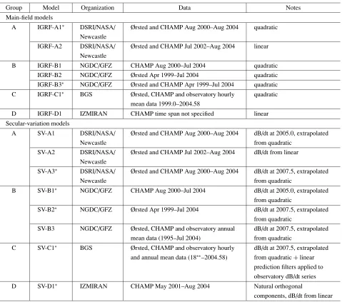
A summary of the data and methods used to generate each model is given in Table 1. Detailed descriptions of all models are given by individual papers in this special issue, namely by Olsenet al.(2005a, b), Mauset al.(2005), Lesur
et al.(2005), and Golovkovet al.(2005).
Table 1. Summary of models. The finally selected models are indicated by an asterisk. SV-B1 and SV-B2 were averaged to provide a single contribution from Group B.
Group Model Organization Data Notes
Main-field models
A IGRF-A1∗ DSRI/NASA/ Ørsted and CHAMP Aug 2000–Aug 2004 quadratic Newcastle
IGRF-A2 DSRI/NASA/ Ørsted and CHAMP Jul 2002–Aug 2004 linear Newcastle
B IGRF-B1 NGDC/GFZ CHAMP Aug 2000–Jul 2004 quadratic
IGRF-B2 NGDC/GFZ Ørsted Apr 1999–Jul 2004 quadratic IGRF-B3∗ NGDC/GFZ Ørsted and CHAMP Apr 1999–Jul 2004 quadratic
C IGRF-C1∗ BGS Ørsted, CHAMP and observatory hourly quadratic mean data 1999.0–2004.58
D IGRF-D1 IZMIRAN CHAMP time span not specified linear Secular-variation models
A SV-A1 DSRI/NASA/ Ørsted and CHAMP Aug 2000–Aug 2004 dB/dt at 2005.0, extrapolated
Newcastle from quadratic
SV-A2 DSRI/NASA/ Ørsted and CHAMP Jul 2002–Aug 2004 dB/dt from linear Newcastle
SV-A3∗ DSRI/NASA/ Ørsted and CHAMP Aug 2000–Aug 2004 dB/dt at 2007.5, extrapolated
Newcastle from quadratic
B SV-B1∗ NGDC/GFZ CHAMP Aug 2000–Jul 2004 dB/dt at 2005.0, extrapolated from quadratic
SV-B2∗ NGDC/GFZ Ørsted Apr 1999–Jul 2004 dB/dt at 2007.5, extrapolated from quadratic
SV-B3 NGDC/GFZ Ørsted, CHAMP and observatory annual dB/dt at 2007.5, extrapolated mean data (1995–Jul 2004) from quadratic
C SV-C1∗ BGS Ørsted, CHAMP and observatory hourly dB/dt at 2007.5, extrapolated and annual mean data (18∗∗–2004.58) from quadratic+linear
prediction filters applied to observatory dB/dt series D SV-D1∗ IZMIRAN CHAMP May 2001–Aug 2004 Natural orthogonal
components, dB/dt from linear
3.
Evaluation of Main-Field Candidates
Evaluating main-field candidates by comparing model predictions with actual measurements turns out to be very difficult. To start with, there exist very few truly indepen-dent vector data. After 2000.0, there were less than 500 vector observations from repeat stations submitted to World Data Centers. Ground observations are valuable in study-ing temporal variations of the geomagnetic field. However, the unknown crustal bias means that their use for evaluating candidate models is limited. Furthermore, the sparse global distribution constrains their information to about spherical harmonic degree 7, while the main-field candidates extend to degree 13.
Instead, we evaluate the models by comparing them at the surface of the Earth as difference maps, compiling tables of root mean square differences, and analyzing their degree and azimuthal power spectra. Four candidate models (one from each Group, selected by the Group) A1, B3, C1 and D1 were compared.
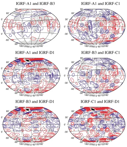
3.1 Maps of MF candidate differences
The candidate models have been compared with each other at the surface of the Earth by plotting differences (Fig. 1) and by computing mean differences for X,Y and
Zon a 2◦latitude/longitude grid (Tables 2–5); note that the latter gives relatively more weight to the polar regions.
The most significant difference between the A1 and B3 model is in the zonal coefficients, due to an ionospheric correction applied to model A1, but not to B3. Even though the g30 (where gm
n is the spherical harmonic coefficient of
degreenand orderm) term is by far the largest coefficient in this correction, the overall effect is roughly that of an inclined g50, as shown in figure 11 of Lowes and Olsen (2004). This zonal pattern is also visible in the comparisons of A1 with C1 and D1. In both cases the amplitude of the differences is larger than that between A1 and B3 and, in addition, there are large differences at northern latitudes, particularly for model D1. In fact, D1 differs strongly from all other models in the polar regions.
180˚-120˚-60˚0˚ 60˚120˚180˚
IGRF-A1 and IGRF-B3
180˚-120˚-60˚0˚ 60˚120˚180˚ -90˚
IGRF-A1 and IGRF-C1
180˚-120˚-60˚0˚ 60˚120˚180˚ -90˚
IGRF-A1 and IGRF-D1
180˚-120˚-60˚0˚ 60˚120˚180˚ -90˚
IGRF-B3 and IGRF-C1
180˚-120˚-60˚0˚ 60˚120˚180˚ -90˚
IGRF-B3 and IGRF-D1
180˚-120˚-60˚0˚ 60˚120˚180˚ -90˚
IGRF-C1 and IGRF-D1
Fig. 1. Differences in the vertical component,Z, at the Earth’s surface between pairs of main-field models. Contour interval: 5 nT, projection: Winkel Tripel.
a 2◦latitude-longitude grid. The results are presented in Ta-ble 2. Summarising the differences by model yields TaTa-ble 3. From Table 3 it can be seen that the differences are reason-ably small for all MF models except for D1, particularly in
Z.
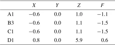
Note that non-zero values for X are due to differences in the zonal harmonics; the non-zero values for Z arise because of the increased weighting in the polar regions. The zero values forY are a check that rounding errors are not significant.
3.2 Lowes-Mauersberger differences between MF
candidates
The mean square (ms) differences between the average fields at the Earth’s surface can be inferred from the differ-ences of the cumulative Lowes-Mauersberger power spectra
(Lowes, 1966).
These differences are illustrated in Fig. 2. MEAN4 is the simple arithmetic mean of the four models. It is clear from Fig. 2 that D1 is the model consistently furthest away from the other three models, and is the model furthest from the mean. Figure 3 gives the values if model D1 is rejected; MEAN3 is the simple arithmetic mean of the remaining 3 models.
A1 B3
D1 C1
64
211 242
248 129
416
A1 B3
D1 C1
49 27
144 107
MEAN4
Fig. 2. Mean square differences between the four primary models and their mean. Unit nT2.
A1 B3
MEAN3
C1 64
47 19
211 129
69
Fig. 3. Differences to the mean if model D1 is rejected. Units are nT2.
Table 2. Mean differences (nT) in MF models on a 2◦latitude-longitude grid at Earth’s surface.
X Y Z F
A1–B3 0.1 0.0 −0.2 0.6
A1–C1 −2.0 0.0 −2.0 −3.6
A1–D1 0.2 0.0 5.2 −0.4
B3–C1 −2.1 0.0 −1.9 −4.2
B3–D1 0.1 0.0 5.3 −1.0
C1–D1 2.2 0.0 7.2 3.2
23 nT2, even though it is based on fewer models. While these assumptions of independence are not strictly valid, this arithmetic indicates that, for whatever reason, model D1 has larger errors than the other three.
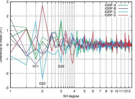
3.3 Spherical harmonic coefficients of MF models For Fig. 4 the MF coefficients of each model were com-pared against the average of the four models A1, B3, C1 and D1, i.e. MEAN4. The abscissa presents the coefficients in the orderg10,g1
1,h11,g20etc. Model groups A and B turn out
to be similar, while C and particularly D exhibit larger dif-ferences to the mean. A spike in coefficientg03 for models A is due to a correction for presumed ionospheric induced fields on the night side, which was not applied by the other groups.
3.4 Main field at the core/mantle boundary
The Lowes-Mauersberger spectrum of the main field is thought to be almost constant at the core/mantle boundary, meaning that there is comparable power in each degree. Only the first degree has significantly larger power, even at the CMB, and is therefore excluded from this analysis.
Table 3. Mean of the mean differences (nT) in Table 2 for each MF model.
X Y Z F
A1 −0.6 0.0 1.0 −1.1
B3 −0.6 0.0 1.1 −1.5
C1 −0.6 0.0 1.1 −1.5
D1 0.8 0.0 5.9 0.6
Two types of power distributions at the CMB are dis-played: the usual distribution of power versus degree, and the distribution of power versus the azimuth, defined as m/n. Figure 5 shows the conventional spectra at the CMB. These spectra look very similar for all models. However, the situation is quite different for the azimuthal power dis-tribution, Fig. 6. The near-zonal (m/n close to 0) coef-ficients of the D1 model have powers which appear erro-neous. In particular, the azimuthal power distribution in all other models is very similar to that for DGRF-2000, while that for D1 implies a change in the field that is unrealistic. 3.5 Evaluation of stated uncertainties of MF
candi-dates
It was requested that all candidate models should be sub-mitted with some measure of coefficient uncertainty. Group C submitted the formal standard deviations (SD) output by the least squares process, Group A adjusted their for-mal SDs upward using empirical variances from a previous study (Lowes and Olsen, 2004), Group B used the differ-ences between two models derived from independent data sets, and Group D did not submit an estimate of uncertainty. Table 4 shows that (unless one model is about right and the other two are much worse), with present modelling techniques, formal standard deviations significantly under-estimate the real uncertainties. The SD under-estimates based on the differences between models using independent data sets are much more realistic.
It is interesting that extending the models fromn = 10 ton =13 does not appear to have added a great deal to the overall model prediction uncertainties (at least at and above the Earth’s surface), despite the large number of extra terms this involves.
3.6 Summary of MF candidate evaluations
-3
erence to mean (nT)
SH degree
Fig. 4. Coefficient differences to the mean of models A1, B3, C1, and D1. The thin lines represent models A2, B1 and B2 which are multiple submissions by the same groups.
1e+10
Fig. 5. Lowes-Mauersberger spectra of models A1, B3, C1, and D1 at the CMB, compared with the spectrum of DGRF-2000.
obviously leads to a slightly different modelling result. This can be due to a variety of sources, particularly ionospheric and induced currents which have different effects on satel-lite and observatory data. Model D1 exhibits significant de-viations from the other models. This was pinned down to a problem in the near zonal coefficients, but the cause is unknown. Indeed, the azimuthal distribution of coefficient powers (Fig. 6) shows that these coefficients deviate more strongly from Models A1, B3 and C1 than did the DGRF-2000. A vote in the IGRF Task Force therefore led to the rejection of Model D1.
4.
Retrospective Evaluation of IGRF-9 Secular
Variation Candidates
In adopting the IGRF-10, an important question was whether the present secular acceleration could be used to predict changes in secular variation forward in time to 2007.5. In other words: is the present secular acceleration a physical characteristic of the field that persists for some time into the future? A retrospective analysis of the candi-dates for the IGRF-9 SV 2000–2005 offers some insight on this issue.
Azimuth m/n (negative for H) IGRF-A IGRF-B IGRF-C IGRF-D DGRF2000
Fig. 6. Azimuthal power density spectrum of models A1, B3, C1, and D1 at the CMB, compared with the DGRF-2000. For these spectra, the SH coefficients of the field at the core-mantle boundary were averaged as a function of their azimuthm/nin bins of 0.2. The extreme bin on either side have a width of only 0.1.
-3 adopted (w/o SV-6) straight average
Fig. 7. Secular variation coefficient differences to the ‘true’ SV in the 2000.0–2005.0 period inferred from the difference between DGRF-2000 and the mean of IGRF-10 candidate models A1, B3, C1, and D1.
Here, we assume that the true SV for 2000.0–2005.0 is given by the difference between DGRF-2000 and the equal average of IGRF-10 MF candidate models A1, B3, C1 and D1, divided by five years.
Table 5 gives the accumulated Lowes-Mauersberger power of the differences of the candidates to the true SV. Figure 7 displays the individual coefficient differences. It can be seen that IZMIRAN-1 was correctly identified as a particularly noisy model which led to its rejection. Also dis-played in Fig. 7 is the adopted model (without IZMIRAN-1), as well as the average of all models.
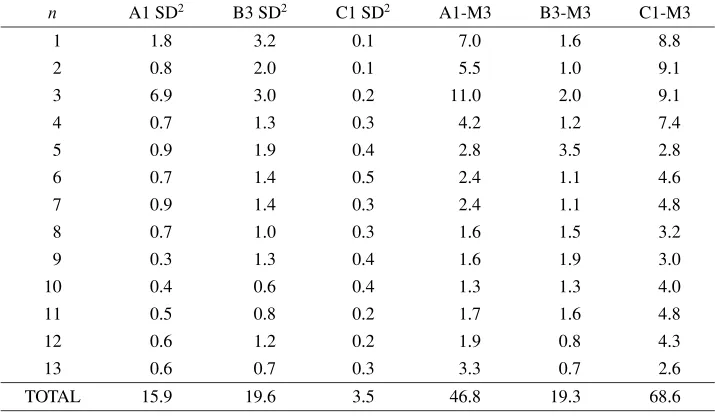
Table 4. Mean square “power” per degree as given by the squares of the stated MF model Standard Deviations, and the differences (Model-MEAN3); unit nT2.
n A1 SD2 B3 SD2 C1 SD2 A1-M3 B3-M3 C1-M3
1 1.8 3.2 0.1 7.0 1.6 8.8
2 0.8 2.0 0.1 5.5 1.0 9.1
3 6.9 3.0 0.2 11.0 2.0 9.1
4 0.7 1.3 0.3 4.2 1.2 7.4
5 0.9 1.9 0.4 2.8 3.5 2.8
6 0.7 1.4 0.5 2.4 1.1 4.6
7 0.9 1.4 0.3 2.4 1.1 4.8
8 0.7 1.0 0.3 1.6 1.5 3.2
9 0.3 1.3 0.4 1.6 1.9 3.0
10 0.4 0.6 0.4 1.3 1.3 4.0
11 0.5 0.8 0.2 1.7 1.6 4.8
12 0.6 1.2 0.2 1.9 0.8 4.3
13 0.6 0.7 0.3 3.3 0.7 2.6
TOTAL 15.9 19.6 3.5 46.8 19.3 68.6
Table 5. Cumulative Lowes-Mauersberger power differences of the IGRF-9 SV candidates to the true SV.
Model Origin/Name Power of difference (nT/a)2 Note
1 BGS 51.6 linear
2 CM3 19.8 B-spline, knot interval 2.5 years
3 OSVM 29.6 linear
4 POMME 17.6 quadratic
5 IPGP 44.4 linear
6 IZMIRAN-1 (rejected) 108.9 linear
7 IZMIRAN-2 41.3 unspecified
Adopted IGRF-9 SV 17.6
compared to the quadratic extrapolation from the possibly less accurate CM3 and early POMME models. This moti-vates the conclusion that accounting for secular acceleration can be more important than model accuracy. In particular, an overall linear SV should be predicted for the centre of the model period, rather than for its start.
Note that the IGRF-10 SV candidates were produced half-way through the 5-year epoch. Unfortunately the fig-ures of Table 5 areonly partly relevant to estimating the accuracy of SV models producedbeforethe beginning of the epoch, as the present ones are.
5.
Evaluation of IGRF-10 Secular Variation
Can-didates
The methods previously applied to the MF candidate models, described above, were also applied to the SV can-didates.
5.1 Differences between SV candidates
As for the MF candidates, component averages were computed on a 2◦latitude-longitude grid at the Earth’s sur-face. The results are displayed in Tables 6 and 7. Model D1 again exhibits the largest mean difference to the other mod-els. However, the maximum bias of 1.5 nT/a in X is rather small and was not considered a major cause for concern.
5.2 Lowes-Mauersberger differences between SV
models
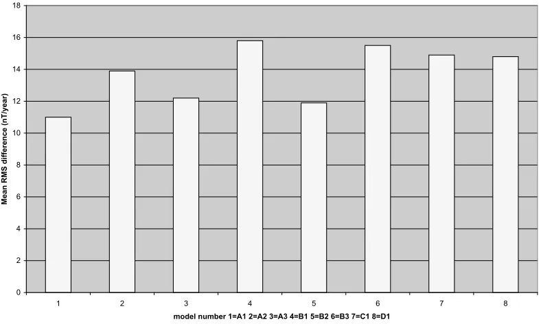
For the SV candidates, it was initially not obvious which models of groups A and B were to be included in the final IGRF SV. Therefore, Fig. 8 displays the average difference of all SV candidates to all other SV candidates. The highest differences were found for the CHAMP-only model B1 and the combined CHAMP/Ørsted/observatory model B3.
The ms vector differences between models was also cal-culated. As for the main field, the comparison was lim-ited to four models: these are the three based mainly on quadratic SV models, A3, B3, C1, and also D1. For the latter, the comparison is not quite fair, as although its background model had a more complicated time variation through the data period, the extrapolation to 2007.5 was lin-ear. The results of this comparison are displayed in Fig. 9; the units are now (nT/a)2, and the sums are taken ton=8. The actual departures from the mean are considerably larger for D1 than for the others. However, this could be partly due to the fact that model D1 gives the SV at 2005.0, whereas the other models predict the SV for 2007.5.
0 2 4 6 8 10 12 14 16 18
1 2 3 4 5 6 7 8
model number 1=A1 2=A2 3=A3 4=B1 5=B2 6=B3 7=C1 8=D1
Mean RMS difference (nT/year)
Fig. 8. Average difference of each SV model with all other SV models.
A3 B3
D1 C1
197
139 346
286 150
365
A3 B3
D1 C1
63 80
157 71
MEAN4
Fig. 9. Mean square differences between four SV models and their mean in (nT/a)2.
In this case, no particular group of models stands out. How-ever, the model B1, based solely on CHAMP data, is quite different from the rest. There are several possible reasons for this difference, in particular:
(1) It could be due to the attitude uncertainty in CHAMP data, even though a correction for this effect was ap-plied
(2) There could be a genuine recent change in the secular acceleration, which is not fully detected by the other models because they either do not include the secular acceleration, or they include data prior to 2000.5.
To investigate possibility (2), an Ørsted-only model using data only after 2000.5 and quadratic variation with time is included as a yellow line in Fig. 10. This model has a higher noise level, probably due to the poorer data coverage of the more recent Ørsted data. However, it appears to confirm the CHAMP result, suggesting that this difference may be due to a genuine shift in secular acceleration prior to 2000.5. A geomagnetic jerk at the end of the 20th century was indeed reported by Mandeaet al.(2000).
5.4 SV at the core/mantle boundary
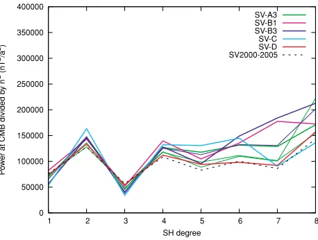
Figure 11 shows the Lowes-Mauersberger spectra of the SV candidates. Since SV spectra are less steep at the Earth’s
surface, and slope upward when downward-continued to the CMB, the SV spectra are further divided by n2for the sole
reason of having comparable expected power levels in all degrees.
The first observation is that the models A1, A2 and D1, which provide SV estimates for 2005.0, generally have lower power. The quadratic extrapolation of the SV into the future by A3, B1, B2, and B3 leads to increased power levels, which is not entirely unexpected. In the case of the C1 model, such an increase was prevented by including out-puts from linear prediction filters applied to long-term data series and by not using the quadratic terms for the degree 7 and 8 coefficients. An increased power level at higher degrees is particularly prominent in the B3 model.
Table 6. Mean differences (nT/a) in SV models on a 2◦latitude-longitude grid at Earth’s surface.
X Y Z
A1–B3 −0.7 0.0 −2.2
A1–C1 −1.7 0.0 −1.1
A1–D1 0.7 0.0 0.0
B3–C1 −1.0 0.0 1.1
B3–D1 1.4 0.0 2.2
C1-D1 2.4 0.1 1.1
Table 7. Mean of the mean differences (nT/a) in Table 6 for each SV model.
X Y Z
A1 −0.6 0.0 −1.1
B3 −0.1 0.0 0.4
C1 −0.1 0.0 0.4
D1 1.5 0.0 1.1
-6 -4 -2 0 2 4
8 7 6 5 4 3 2
1
Diff
erence to mean (nT)
SH degree H11
G22
CHAMP
CHAMP
H33
SV-A SV-B Oersted after 2000.5 SV-C SV-D
Fig. 10. Secular variation coefficient differences to the mean of models A1, B3, C1, and D1. The thin lines represent models A2, A3, B1 and B2 which are multiple submissions by the same groups. The model labelled CHAMP is the B1 model estimated from CHAMP measurements only. The yellow line is a model from only Ørsted data of the same period as the CHAMP data.
5.5 Evaluation of stated uncertainties of SV candidate models
As for the MF candidate models, Group C submitted the formal SDs output by the least squares process, Group A adjusted these upward using empirical variances from a previous study (Lowes and Olsen, 2004), Group B used the difference between two models from independent data sets, and Group D did not submit any estimate of uncertainty.
The power 248 (nT/a)2as given for B3 as SD2 in Table 8 (based on the differences between B3 (Ørsted+CHAMP+ observatories) and the individual models B1 (CHAMP) and B2 (Ørsted)) is a lot larger than the 148 (nT/a)2ms
differ-ence between B1 and B2, so the addition of only 8% of ob-servatory data has moved the B3 model significantly away
0 50000 100000 150000 200000 250000 300000 350000 400000
1 2 3 4 5 6 7 8
P
o
w
er at CMB divided b
y n
2 (nT 2/a 2)
SH degree
SV-A3 SV-B1 SV-B3 SV-C SV-D SV2000-2005
Fig. 11. Lowes-Mauersberger spectra, further divided by n2, of SV models A3, B1, B3, C1, and D1 at the CMB, compared with the true SV from 2000–2005. Thin lines represent models A1, A2 (green) and B2 (blue).
0 5000 10000 15000 20000 25000 30000
-1 -0.5 0 0.5 1
P
o
w
er at CMB divided b
y n
2 (nT 2/a 2)
Azimuth m/n (negative for H)
SZ-A3 SV-B1 SV-B3 SV-C1 SV-D1 SV2000-2005
Fig. 12. Azimuthal distribution of powers in SV models A1, B1, B3, C1, and D1 at the CMB, compared with the true SV from 2000–2005. Thin lines represent models A1, A2 (green) and B2 (blue).
from the mean of satellite models B1 and B2. And B3 SD2 seems to be about 4 times too large (for variances) com-pared with the scatter of the three models. In contrast, de-spite the substantial scaling of the A3 variances they are still too small, by a factor of about 10; the (formal least-squares) variances of C1 are 10 times smaller still! As detailed for the main field models, with present modelling techniques, formal standard deviations very much under-estimate the real uncertainties.
5.6 Summary of SV candidate evaluations
The comparison of SV models shows that model D1 is most different from the other models. The straight-forward extrapolation via quadratic terms used for models A3, B1, B2, and B3 generally lead to larger SV powers at higher degrees. Models A1, A2 and D1, essentially giving the present SV, have the lowest powers. For model C1, the quadratic SV was not used for degrees 7 and 8, which allowed for an extrapolation without increasing the power at these higher degrees.
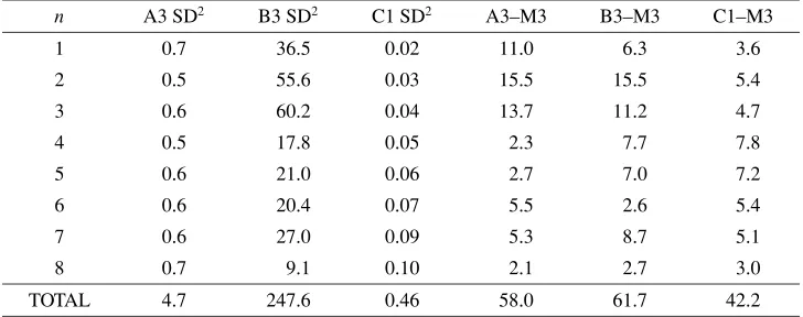
Table 8. Mean square “power” per degree as given by the squares of the stated SV model Standard Deviations, and the differences (Model-MEAN3), where MEAN3 is the average of A3, B3, C1; unit (nT/a)2.
n A3 SD2 B3 SD2 C1 SD2 A3–M3 B3–M3 C1–M3
1 0.7 36.5 0.02 11.0 6.3 3.6
2 0.5 55.6 0.03 15.5 15.5 5.4
3 0.6 60.2 0.04 13.7 11.2 4.7
4 0.5 17.8 0.05 2.3 7.7 7.8
5 0.6 21.0 0.06 2.7 7.0 7.2
6 0.6 20.4 0.07 5.5 2.6 5.4
7 0.6 27.0 0.09 5.3 8.7 5.1
8 0.7 9.1 0.10 2.1 2.7 3.0
TOTAL 4.7 247.6 0.46 58.0 61.7 42.2
Force finally voted for a mix of A3 (25%), B1 (12.5%), B2 (12.5%), C1 (25%) and D1 (25%).
6.
Conclusions
The recent satellite magnetic missions CHAMP and Ørsted, together with observatory data, have provided the basis for a highly accurate main-field model for 2005.0, and a reasonably accurate secular-variation model for the 2005.0–2010.0 epoch. Based on the scatter of the candidate models, the adopted IGRF for 2005.0 has a formal variance of 23 nT2, corresponding to a very low vector standard
devi-ation over the Earth’s surface of less than 5 nT, a significant improvement over previous epochs. However the various assumptions involved in producing such a formal estimate are almost certainly not valid; past experience has shown that such estimates almost always under-estimate the true error. The actual standard deviation might well be 10 nT or more.
Due to the inherent uncertainty in secular variation fore-casts, the relative accuracy of the adopted SV is very much poorer. Based on the scatter of the contributing models, the formal variance of the adopted SV model is only about 25 (nT/a)2, corresponding to an rms vector uncertainty over the Earth’s surface of 5 nT/a. Again such a formal estimate ignores many problems; comparison of previous IGRF pre-dictive SVs with what actually happened shows that in the past a typical error was 25 nT/a. Hopefully the use of satel-lite data will give some improvement, but as yet we do not know how much. We suggest 20 nT/a as a conservative fig-ure for the current IGRF-SV.
Attempts to verify models by comparison with real data invariably remain inconclusive. The main reason is that the candidates are derived from very large sets of data. Com-paring these candidates with small subsets of data generally leads to misfits which are much larger than the actual dif-ferences between the candidates. This is due to local custal and induced fields, as well as unmodeled external fields.
While comparisons with real data may seem appealing, evaluation strategies can be based on comparing candidates with each other and with models of the previous epoch. Several different such strategies have been pursued here.
These methods complement each other and this paper may serve as a reference for future IGRF candidate evaluations.
Finally, it is also interesting to make retrospective evalua-tions of the candidate models for the previous IGRF round. For IGRF-9, it was found that one factor for successfully modelling SV for 2000–2005 was to use quadratic polyno-mials in time. Even though the IGRF-9 candidates were submitted at 2003.2, hence, after the centre of the epoch, this finding motivated the Task Force to adopt an SV model for which 75% of the candidates extrapolated the SV using quadratic terms to 2007.5, while 25% of the SV stems from model D1 giving the SV at 2005.0. It will be interesting to see by a retrospective evaluation in 2010 whether this con-fidence in quadratic terms turns out to be justified.
References
Golovkov, V. P., T. I. Zvereva, and T. A. Chernova, The IZMIRAN main magnetic field candidate model for IGRF-10, produced by a spherical harmonic-Natural orthogonal component method,Earth Planets Space, 57, this issue, 1165–1171, 2005.
Lesur, V., S. Macmillan, and A. Thomson, The BGS magnetic field candi-date models for the 10th generation IGRF,Earth Planets Space,57, this issue, 1157–1163, 2005.
Lowes, F. J., Mean-square values on sphere of spherical harmonic vector fields,J. Geophys. Res.,71(8), 2179, 1966.
Lowes, F. J. and N. Olsen, A more realistic estimate of the variances and systematic errors in spherical harmonic geomagnetic field models,
Geophys. J. Int.,157(3), 1027–1044, 2004.
Mandea, M., E. Bellanger, and J.-L. Le Mou¨el, A geomagnetic jerk for the end of the 20th century?,Earth Planet. Sci. Lett.,183, 369–373, 2000. Maus, S., S. McLean, D. Dater, H. L¨uhr, M. Rother, W. Mai, and S. Choi,
NGDC/GFZ candidate models for the 10th generation International Ge-omagnetic Reference Field,Earth Planets Space,57, this issue, 1151– 1156, 2005.
Olsen, N., F. Lowes, and T. J. Sabaka, Ionospheric and induced field leak-age in geomagnetic field models, and derivation of candidate models for DGRF 1995 and DGRF 2000,Earth Planets Space,57, this issue, 1191–1196, 2005.
Olsen, N., T. J. Sabaka, and F. Lowes, New parameterization of exter-nal and induced fields in geomagnetic field modeling, and a candidate model for IGRF 2005,Earth Planets Space,57, this issue, 1141–1149, 2005.