R E S E A R C H
Open Access
Efficient two-dimensional compressive
sensing in MIMO radar
Nafiseh Shahbazi
1*, Aliazam Abbasfar
1and Mohammad Jabbarian-Jahromi
2Abstract
Compressive sensing (CS) has been a way to lower sampling rate leading to data reduction for processing in multiple-input multiple-output (MIMO) radar systems. In this paper, we further reduce the computational complexity of a pulse-Doppler collocated MIMO radar by introducing a two-dimensional (2D) compressive sensing. To do so, we first introduce a new 2D formulation for the compressed received signals and then we propose a new measurement matrix design for our 2D compressive sensing model that is based on minimizing the coherence of sensing matrix using gradient descent algorithm. The simulation results show that our proposed 2D measurement matrix design using gradient decent algorithm (2D-MMDGD) has much lower computational complexity compared to one-dimensional (1D) methods while having better performance in comparison with conventional methods such as Gaussian random measurement matrix.
Keywords:Compressive sensing, Measurement matrix, Multiple-input multiple-output (MIMO) radar, Sensing matrix, Two-dimensional sparse signal model
1 Introduction
Compressive sensing (CS) is a signal processing method for reconstructing a signal that is sparse in a specific domain [1, 2]. In the past two decades, much research in various disciplines such as mathematics, statistics, signal processing, and communication systems has been conducted in CS topic in order to exploit its advantages for a wide range of applications. For example, analog-to-information conversion [3], remote sensing [4], channel estimation in the communication systems [5], medical imaging [6], and image reconstruction [7] are some of these applications.
In CS, the main goal is to find the sparsest vector s that satisfies an underdetermined system of linear equa-tionsy=ΦΨs, in which the number of variables is much larger than the number of equations, where y is the measurement vector,Φ is the measurement matrix, and Ψ is the basis matrix. It can be formulated in mathe-matic language as, minimize ‖s‖0, subject to y = ΦΨs,
where‖⋅‖0is l0-norm andA=ΦΨis called the sensing
matrix. Thel0-norm calculates the number of non-zero
components of a vector. To solve this problem, we need a combinatorial search to find the minimum l0-norm,
which is an NP-hard problem. One of the solutions proposed for this problem is to replace l0-norm with l1-norm and convert the problem to a convex one. A
famous algorithm that minimizes l1-norm is basis
pur-suit (BP) [8].
Some applications of compressive sensing in radar systems have been recently studied in [9–11]. In [12], the direction of arrival (DOA) of the signal is estimated using CS for communication systems. In order to esti-mate the desired parameters in CS radar, it should be assumed that the number of targets to be found is much smaller than the whole number of radar bins, which is the case in most practical radar applications.
Multiple-input multiple-output (MIMO) radar systems have received the attention of many researchers in re-cent years. There are two different types of MIMO radar systems which are categorized according to their anten-nas configuration. In the first type, the antenanten-nas are widely separated from each other relative to their dis-tance to the target [13]. In the second one, which is con-sidered in this paper, the antennas are collocated and located close to each other [14].
* Correspondence:[email protected]
1School of Electrical and Computer Engineering, University of Tehran, Tehran, Iran
Full list of author information is available at the end of the article
In [15], the sparse signal model of MIMO radar is derived using only one incoming pulse. Furthermore, a sparse learning via iterative minimization (SLIM) algorithm is developed and compared to other sparse methods such as iterative adaptive approach (IAA) [16]. The main drawback of SLIM algorithm in [15] is that its compu-tational complexity will be very high for pulse-Doppler MIMO radars.
Recently, a new signal model with two-dimensional (2D) sparse parameters, called 2D sparse signal model, has been introduced [17, 18], and some algorithms for 2D sparse reconstruction have been proposed [19–24]. Specifically, in [19], the 2D version of IAA is derived in which its computational cost is drastically reduced in comparison with the one-dimensional (1D) IAA. The other 2D sparse recovery algorithm is the smoothed L0 (SL0) algorithm that minimizes an approximated l0
-norm function [20] and has much lower computational complexity than its 1D counterpart. In [21], a 2D sparse signal model for a radar is obtained and solved by 2D-SL0 algorithm with acceptable results. Also, 2D-SLIM [22], 2D Truncated Newton Interior Point Method (2D-TNIPM) [23], and 2D Sparse Bayesian Learning using Laplace Prior (2D-SBL-LP) [24] have been proposed for pulse Doppler MIMO radars. These papers have demon-strated that the 2D proposed algorithms have much less computational complexity compared to corresponding 1D sparse recovery algorithms.
The main goal of sparsity-based methods for MIMO radar systems ([21–24]) is to achieve accurate estimates for target parameters, whereas in this paper, we mainly focus on the CS MIMO radar problem to reduce the sampling rate lower than the Nyquist criterion by de-signing a suitable measurement matrix. Therefore, the main difference between our 2D CS MIMO radar signal model and 2D sparse model in [21–24] is that we con-sider the measurement matrices in our model in which these measurement matrices can be applied on receivers and received pulses, separately.
In [18], a 2D CS signal model has been proposed for inverse synthetic aperture radar (ISAR) imaging radar in which a random sub-sampling in both range and azimuth dimensions is utilized. Also, a 2D CS image reconstruction algorithm based on iterative gradient projection is derived in [25].
Compressive sensing for MIMO radar systems is proposed and analyzed in [26, 27]. A MIMO radar, which is one of the most practical applications of MIMO systems, transmits some independent wave-forms by its transmit antennas and has superior spatial resolution compared to traditional radar systems. CS in MIMO radar has the ability to achieve the same localization performance as the traditional methods while using much lower number of measurements,
which is achieved by applying a measurement matrix to the normally measured samples.
In CS, the measurement matrix has a key role in the performance of sparse signal recovery algorithm. Therefore, we can improve the performance of target detection in CS MIMO radar by designing a suitable measurement matrix. The conventional approach for choosing this matrix is a Gaussian random measurement matrix (GRMM) which is not necessarily the best one for CS. According to [28], if themutual coherence(MC) that is the maximum value of pairwise correlation among the columns ofAis small, the sparse signal can be recovered with high probability. Re-cently, some measurement matrix design methods have been proposed based on minimizing the MC of the sensing matrix [29–31]. Elad [29] designed the measurement matrix based on mutual coherence minimization using a shrinkage operation. Duarte-Carvajalino [30] optimized the meas-urement matrix and basis matrix jointly by a KSVD-based algorithm. However, these methods are adapted for real signals and also have many parameters that should be set properly.
In [31], a gradient descent method is used to minimize the MC of A which is described as the absolute off-diagonal elements of the Gram matrix. It is shown that this method can achieve higher sparse reconstruction performance compared to previous methods. In our paper, we extend this method to a complex CS MIMO radar signal and decrease the computational complexity by proposing a 2D CS MIMO radar signal model. In [32], a method for optimizing the measurement matrix of MIMO radar systems is proposed based on two differ-ent criterions; first one is to minimize the summation of coherence of cross columns in the sensing matrix plus maximize the signal-to-interference ratio (SCSM + SIR), and the second criterion is to maximize SIR by imposing a special structure on the measurement matrix. How-ever, both methods are suboptimal solutions and may not have acceptable performance in different situations.
In this paper, we introduce a 2D signal model in CS for a collocated MIMO radar with point targets, and then we improve the efficiency of this 2D MIMO radar model by proposing a measurement matrix design using gradient decent algorithm (MMDGD) in which the MC of sensing matrix is minimized. We call the proposed method as 2D-MMDGD.
consequently better performance compared to its initial value, i.e., GRMM. Simulation results show that our pro-posed 2D-MMDGD performs much better than GRMM, SIR, and SCSM + SIR methods.
The rest of the paper is organized as follows. Sections 2 and 3 describe the 1D and 2D CS signal model of the MIMO Radar, respectively. In Section 4, we propose a measurement matrix design for 1D and 2D CS model using gradient decent algorithm. The computational complexity of the proposed methods is discussed in Sec-tion 5. SimulaSec-tion results are given in secSec-tion 6. Finally, we have conclusions in section 7.
Notations: Lower case and capital letters in bold de-note vectors and matrices. Superscripts (.)T, (.)H denote the transpose and Hermitian transpose of a matrix, re-spectively. 0M×Ndenotes an M×Nmatrix with all zero elements and INdenotes an N×Nidentity matrix. Also, ‖.‖2and ‖.‖Fdenote the square and Frobenius norm of a vector/matrix, respectively. The operator⊗, var(.), and
E(.) are the Kronecker product, variance, and expect-ation of a random variable, respectively.
2 1D-CS signal model of MIMO radar
In this section, we describe the 1D signal model of a CS pulse-Doppler MIMO radar. In this model, we assume that one period of Doppler frequencies of targets spans a duration of several received pulses. It means thatfdτ≪1,
where fdand τare the Doppler shift frequency and the
pulsewidth, respectively. If fc is the carrier frequency,
this assumption can be written asfr≪B≪fc, wherefris the radar pulse repetition frequency (PRF) and B is the bandwidth of the transmitted signal. Based on this as-sumption, the Doppler effect on each pulse is simply a phase shift. We assume that Doppler shift frequency is in the interval −fr
2 ; fr
2
h
and the targets are located behind
the maximum unambiguous range. Suppose that the Doppler frequency of interest divided intoNdbins:
fd ¼− Doppler phase shift over one pulse period for the dth Doppler bin is obtained as
θd ¼
2πfd
fr
ð2Þ
The transmitted signal samples of all antennas can be put together in a matrix as
V¼ ½v1⋅⋅⋅vMt ð3Þ
where vi∈ℂL× 1, i= 1,…,Mt is the samples of the
transmitted signal with lengthL by the ith antenna (for a total ofMttransmit antennas).
Without loss of generality, a uniform linear array for the transmit and receive antenna arrays has been used in our model and simulations in this paper.
Suppose that the number of range bins is Nr in the
radar surveillance area, then the largest possible delay between the transmit and receive pulses is (Nr−1).
We consider the number of the angle bins of the an-tenna array to beNaand the angle bins aref gαa Na¼a1. The
transmit and receive antenna array steering vectors of the ath angle bin are shown, respectively, as aa∈CMt1,
where Δt and Δr are the distance between elements of transmit and receive antennas, respectively, andλ0is the signal of transmitting wavelength.
The compressed received signal in the mth antenna returned from thepth transmitted pulse can be arranged in an observation vector,ypm∈ℂM (compressed observations), the number of pulses, and receive antennas, respectively. It is noted that for com-pressive sensing scenario, we haveM<~L.
The vector npm=φpmepm is the additive noise for the
mth receive antenna andpth pulse and epm∈ℂL~1 is the
receiver noise with complex Gaussian random distribu-tion, with zero mean and covariance matrix IL~. As it is noted, the noise covariance matrixnpmisφpmφHpm.
The matrix Jr∈ℂL~L is a time-shift matrix which
Jr¼ …,Nd) denote the return coefficients from targets in the radar interest area, wheresr,a,d=βkif thekth target is lo-cated at the (r,a,d)th bin andsr,a,d= 0 otherwise. In gen-eral,βkis a complex number corresponding to the radar cross section of thekth target (k= 1, 2,…,Nt), andNtis
the number of targets.
Now, the received signal samples from themth receive antenna returned from thepth transmitted pulse can be written as the basis matrix for themth receiver during thepth pulse,
⊗is the Kronecker multiplication, and hm rð;aÞ¼JrVaae−
We can also arrange the observations for all receive antennas for thepth pulse in vector formyp∈ℂMMr1as agonal matrix in which themth block is a measurement matrix used formth receive antenna and defined as
Tp ¼blkdiag φp1; φp2;…; φpMr
∈ℂMMrLM~ r: ð15Þ The matrixΨpin (14) which is the basis matrix for all antennas, and thepth pulse is defined as
Ψp¼
For all the pulses, we have
y¼ yT
the measurement matrix which is applied to all observations in order to decrease the number of re-ceived signal samples, Ψ¼ΘT⊗H∈ℂ~LMrNpN is the
basis matrix for our pulse-Doppler MIMO radar system, Θ¼½θ1 ⋯ θNP∈ℂ
NdNp is the MIMO radar
diction-ary matrix containing the Doppler information of targets in different situations, and n¼Φe∈ℂMMrNp1 is the additive
noise of all receivers and pulses after compression, wheree¼ eT1 ⋯ eTNp
h iT
. The matrixHis defined as
H¼ matrix containing the whole range and angle informa-tion of targets. Also,Ψcan be given by:
Ψ¼
Our goal in this paper is to design the measurement matrixΦ such that the CS MIMO radar has better per-formance in target detection compared to conventional approaches.
To optimizeΦ, four different cases can be considered:
Case 1(general case): All sub-blocksφpm(p= 1,…,Np and m= 1,…, Mr) located in Φ are different with each other, and thus, they are optimized, separately.
Case 2: We assume that the measurement matrix is equal for all receivers,
φp1¼φp2¼…¼φpMr ¼φp: ð20Þ
Therefore, Tp ¼IMr⊗φp , where φp∈CM~L is the measurement matrix applied on the pth received pulse, andΦ¼blkdiag T1; T2; …; TNp
∈ℂMMrNpLM~ rNp.
Case 3: We assume that the measurement matrix is equal for all received pulses,
φ1m ¼φ2m¼…¼φNpm¼φm ð21Þ
where φm∈CML~ is the measurement matrix applied on the mth receive antenna; therefore, Φ¼INp⊗T, where T¼blkdiagðφ1;φ2;…;φM
rÞ.
Case 4: We assume that the measurement matrix is equal for all receivers and pulses,
φ11¼φ12 ¼…¼φNpMr¼φ: ð22Þ
Therefore, we have Φ¼INp⊗T, where T¼IMr⊗φ,
3 2D-CS signal model of MIMO radar
In this section, we derive the 2D-CS signal model for MIMO radar and explain its relationship to the classical 1D-CS signal model.
Among all cases discussed in the last section, only case 3 and case 4 can be converted to 2D model. To do so, we arrange the received signals for all pulses into a matrix as
Y¼ y1 ⋯ yNP
¼THSΘþN ð23Þ
where S¼ sT
1 sT2 … sTNd
, N=TΕ, and Ε¼ e1 ⋯ eNP
½ . This equation is the 2D model of CS MIMO radar. We can present the relationship be-tween 1D and 2D sparse signal model for MIMO ra-dars transmitting a trail of pulses by using the following property [33]:
vecðTHSΘÞ ¼ΘT⊗THvecð ÞS ð24Þ
If we apply Eqs. (24) to (23), we re-derive the 1D CS model shown in Eq. (17), where we have
y¼vecð ÞY ; s¼vecð ÞS ; n¼vecð ÞN ð25Þ
and
A¼ΦΨ¼ΘT⊗TH∈ℂMMrNpN: ð26Þ
Also, we can rewrite matrixAas a block matrix whose
pmth block is the measurement matrix φpm applied on
pth received pulse and mth receive antenna multiplied bypmth basis matrixψpm:
A¼ A11
A12
⋮
ANpMr
2 6 4
3 7 5¼
φ11ψ11
φ12ψ12
⋮
φNpMrψNpMr
2 6 4
3 7
5: ð27Þ
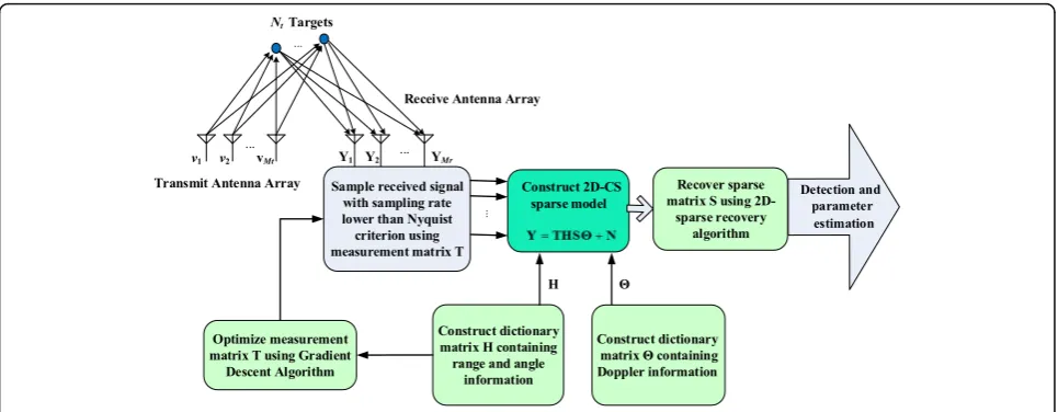
Figure 1 shows the block structure of the 2D-CS signal model implementation for MIMO radar. As noted be-fore, two dictionary matrices H and Θ are constructed based on potential situations of range, angle and Dop-pler frequency of targets in MIMO radar surveillance area. Also, the sampling of signal is conducted based on measurement matrixTwhich is optimized in the follow-ing section usfollow-ing gradient descent algorithm.
4 Measurement matrix design using gradient decent algorithm for CS model
In this section, first we discuss the conditions that a measurement matrix should have, and then we propose a new measurement matrix for CS MIMO radar that is suitable for our 1D and 2D CS models.
The mutual coherence (MC) of sensing matrix A that shows the maximum value of the pairwise correlations of the column vectors ofAis defined as follows [28]
μð Þ ¼A max
i≠j
ρi;j ai
k k2 aj 2
ð28Þ
where ρi;j¼ aHi aj and ai is the ith column of A. The mutual incoherence property (MIP) is one of the best conditions for sparse signal reconstruction [28]. Accord-ing to the MIP, for a small value ofμ(A), the sparse sig-nal can be reconstructed with high probability. In fact, the exact reconstruction of s will be guaranteed if the following inequality holds [29]:
s0
The statistical analysis of MC of sensing matrix is per-formed in Appendix 1 for the aforementioned four cases. The following results are concluded:
Eðμcase 1Þ ¼Eðμcase 2Þ ¼Eðμcase 3Þ ¼Eðμcase 4Þ ð30Þ
varðμcase 1Þ≤varðμcase 3Þ≤varðμcase 4Þ ð31Þ varðμcase 1Þ≤varðμcase 2Þ≤varðμcase 4Þ: ð32Þ
As it is seen, case 1 has the least variance of MC, and therefore, it is expected that it has better performance compared to other cases. On the other hand, case 4 has the biggest variance of MC, and therefore, it is expected that it has the worst performance.
Also, as shown in [34], (28) might not have a good behav-ior for the case that coherence of cross columns is small. In [29], Elad proposes the average mutual coherence as an al-ternative criterion because of its lower computational com-plexity compared to (28). Therefore, the new measurement matrix optimization can be expressed as:
Φ^¼arg min
Φ ∥G−IN∥
2
F ð33Þ
whereG is the Gram matrix defined asG=AHA. Thus, we propose an algorithm to decrease the mutual coher-ence ofAwhich is determined by minimizing the whole elements ofGexcept the main diagonal elements.
4.1 Measurement matrix design for 1D-CS model
As mentioned before, among the four cases we dis-cussed, cases 1 and 2 cannot be converted to 2D model. We consider the optimization of these two cases as measurement matrix design for 1D-CS model.
Therefore, the following cost function can be defined for our problem:
Thus, the optimization problem is formulated as ^
Φ ¼arg min
Φ C.
In our proposed method, first we optimize matrix A using gradient descent algorithm [31], then the measure-ment matrixΦis obtained formAby using least square (LS) estimator. In the gradient descent method, the gra-dient of cost function Cneeds to be computed with re-spect to the unknown variableA, denoted as
∇C¼∂∂CA¼4A A HA−IN ð35Þ then, the equationA=A−η∇Cis updated in an iterative
process, where η> 0 is the stepsize that can be fixed or updated iteratively by backtracking line search algorithm [35]. Before the execution of descent algorithm, the col-umns of matrixAneed to be normalized as:
ai¼ai=k kai 2: ð36Þ
The algorithm can be stopped when the stopping cri-terion ‖∇C‖F≤ε for a small and positive constant ε or after a several number of iterations (NGD).
4.1.1 Case 1
After obtainingAfor case 1, the measurement matrix of
pth pulse andmth receiver (φpm) is given by solving the following linear equation:
Apm¼φpmψpm ð37Þ
whereApmis defined in (27). From Eqs. (6) to (13), it can be noted that some parts of matrixψpmis filled with 0, and consequentlyψH
pmψpm tends to be ill-conditioned.
Therefore, the LS estimator which needs to calculate
ψH pmψpm
−1
cannot be exploited, directly. To resolve
this problem, we use the economy-size singular value decomposition (eSVD) ofψpm∈ℂL~Ngiven by ris the number of non-zero singular values ofψpm. The measurement matrixφpmcan be obtained as follows:
φbpm ¼ U1;pm Δ−1
Table 1 shows all the steps of the proposed method for optimizing measurement matrix in case 1.
4.1.2 Case 2
4.2 Measurement matrix design for 2D-CS model
In our 2D-model, we haveA=ΘT⊗B, whereB=TH. It is demonstrated in Appendix 2 that the MC ofAis equal to
μð Þ ¼A μΘTμð ÞB ð41Þ According to (41), to optimize measurement matrixT based on minimizing μ(A) with respect to T, it is only
needed to minimize μ(B) with respect to T. Therefore, the optimization problem becomes:
^
T ¼ arg min
T ðTHÞ
HTH−I NrNa
2
F ð42Þ
By using gradient descent optimization algorithm for cost function C¼BHB−INrNa
2
F, we can obtain
B∈ℂMMrNrNa similar to 1D model.
4.2.1 Case 3
In this case, the measurement matrix is equal for all re-ceived pulses. After obtaining B, the measurement matrix ofmth receiver (φm) is calculated by solving the following linear equation:
Bm¼φmHm ð43Þ
whereB¼ B1
B2
⋮
BMr
2 6 4
3 7 5.
Similar to case 1, the eSVD of Hm is computed, and thenφmis calculated.
4.2.2 Case 4
As noted for case 4, the measurement matrix is equal for all received pulses and receivers, i.e., T¼IMr⊗φ. Therefore, we can use the redundant data of all re-ceivers in optimization of measurement matrix φ. To do so, the linear equation B=TH should be reshaped to Be¼φHe, where Be∈CMMrNrNa is the reshaped form of B∈CMMrNrNa, and
H
~
¼ ½H1H2…HMr∈CL
eMr Nr Na: ð
44Þ
Now, the eSVD of He∈CLeMrNrNa is computed as follows:
H
~
¼U4Δ4 0
0 0
! DH
4 ð45Þ
where U4∈ℂL~L~ and D4∈ℂMrNrNaMrNrNa are unitary
matrices andΔ4= diag(λ'1,…,λ'r) is the singular values matrix of H that λ'i≠0 for i= 1,…, r. Also, r is the number of non-zero singular values ofH. The measure-ment matrixφcan be given as follows:
φb¼
"
U4 Δ−41 0
0 0
! DH
4B
~
H#H : ð46Þ
Table 2 shows all the steps of the proposed method to optimize measurement matrix in case 4. In this table, bi is theith column ofB.
Table 1Designed measurement matrix algorithm for 1D
5 Computational complexity comparison
The cases 1 and 2, called 1D proposed MMDGD methods, have almost the same computational complexity because the gradient descent algorithm for calculating matrixAis
the same for both cases. Also, the computational complex-ity of cases 3 and 4, called as 2D proposed MMDGD methods, are almost equal due to the similarity of their gradient descent algorithm. The main computational cost in each iteration of 1D and 2D proposed MMDGD methods belong to matrix product AAHA and BBHB, respectively. The complexities ofAAHAandBBHBare O
M2M2rN2pN
and O M2M2rNrNa
¼O M2M2rN=Nd
,
respectively. Thus, the ratio of 2D-MMDGD load over that of its 1D equivalent is 1
N2 pNd.
The complexity of SCSM + SIR method that uses CVX package to optimize measurement matrix is
OðNe3Þ, whereNe¼Le2[35]. It can be approximated that
OðM2M2
rNrNaÞ≪OðLe 6
Þ due to the facts that M≪Le,
Na≈Nr<Le, andMr<Le in our application. Therefore, the computational complexity of our proposed 2D-MMDGD is much less than the SCSM + SIR method.
The computational complexity of 1D and 2D sparse recovery algorithms are discussed in [22] and [24]. As noted there, the computations of 1D and 2D algorithms for CS are O(MMrNpN) andO(MMrN) +O(MMrNpNd), respectively. Therefore, the ratio of 2D processing load over that of its 1D equivalent is 1
Npþ
1 NaNr.
In the next section, CPU time is used as a rough esti-mate of computational complexity of the algorithms.
6 Simulation results
For simulation, we consider a pulse-Doppler MIMO radar withMttransmit (TX) andMrreceive (RX) anten-nas having uniform linear array (ULA) with Δt= 2.5λ0
and Δr= 0.5λ0. The transmitted waveforms are obtained
from efficient cyclic algorithm [36] that can produce sequences with very low auto- and cross-correlation sidelobes. We consider the length of sequence L= 32 with unit power. The number of transmit and receive antennas are Mt= 3 and Mr= 3, respectively. The
number of pulses is Np= 3. The carrier frequency, the pulse bandwidth, and PRF are fc= 1 GHz, B= 10 MHz, and fr= 2kHz, respectively. The area under the radar includes Nr= 6 range bins, Nd= 6 Doppler bins, and
Na= 6 angle bins between 0° to 35° with 7° resolution. We use the 1D-SLIM [15] and 2D-SLIM [22] algo-rithms to reconstruct ŝ and Ŝ from the received com-pressed measurements in (17) and (23). Over 100 independent trials were run. In each trial, the locations of targets are generated randomly following a uniform random distribution.
The signal-to-noise ratio (SNR) is defined for each tar-get located at the (r,a,d)th range-angle-Doppler bin and the noise varianceσ2as
Table 2Designed measurement matrix algorithm for 2D model
SNR¼10 log10 sr;a;d
2
=σ2
: ð47Þ
The SNRs of all targets are considered equal.
At first, we compare the performance of four cases when the GRMM is used. In fact, GRMM is a com-plex Gaussian random matrix with zero mean and covariance matrix I. The reconstruction error (k^s−sk22
=k ks 2
2) for all cases versus the number of
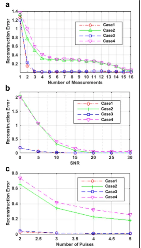
measure-ments, SNRs, and the number of pulses are shown in Fig. 2a–c, respectively, where ŝ and s are the esti-mated and true vectors containing the return complex reflection coefficients of targets, respectively. As seen in these figures, cases 1 and 3 have almost the same reconstruction error while outperforming two other cases.
It can be concluded from the simulation results that case 3 is the best choice for MIMO radar under the con-dition of low SNR, small number of measurements, and pulses. The reason is that the reconstruction error of case 3 is less than that of cases 2 and 4 while it is as small as the reconstruction error of case 1. It should be noted that the computational cost of case 3 is much less than that of case 1 as shown in Section 5.
As depicted in these figures, by increasing the num-ber of measurements, SNRs, and numnum-ber of pulses, the reconstruction errors of cases 2 and 4 decrease and get close to cases 1 and 3. As a result, under the condition of high SNR, large number of measure-ment, and pulses, case 4 can be considered for MIMO radar due to its ease of implementation. By the above discussion, one can easily find the effective-ness of our 2D proposed MMDGD methods com-pared to 1D ones.
The convergence of the gradient descent algorithm is demonstrated for convex and non-convex problems in [35] and [37, 38], respectively. Here, to show the conver-gence rate of the proposed method, we define the RMSE of convergence curve askBðjþ1Þ−Bð Þjk2F, wherejis the iteration index.
Figure 3 shows the convergence curve of this algo-rithm for our proposed measurement matrix design for 500 Monte Carlo runs. As it is clear, the proposed algo-rithm can converge after 20 iterations for M= 4 and after 40 iterations forM= 8.
Now, we compare the detection performance of the proposed method with GRMM, SIR, and SCSM + SIR methods using receiver operating characteristic (ROC) curve. Since in the SIR and SCSM + SIR methods, the measurement matrix is designed only for case 4 (because this matrix optimization will be very time consuming for
Fig. 2Reconstruction error of four cases versusathe number of
cases 1, 2, and 3 especially in SCSM + SIR), we consider only case 4 for comparison with these two methods.
In ROC curve, the probability of detection (Pd) is
plot-ted versus the probability of false alarm (Pf). We
con-sider any local maximum of the absolute value ofSthat is larger than a selected threshold τi as a target. Then,
we vary the threshold τi within an interval [τLτH] and for each τi, we count the number of detected actual or false targets. The empirical probability of detection Pd
of actual targets and the empirical probability of false alarm Pf of false targets for different values ofτi is ob-tained by repeatingNitrtrials of the experiment as:
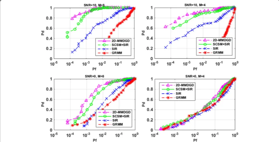
Fig. 4Comparison of ROC curves for different measurement matrix in CS MIMO radar (resolution 7°)
Pd ¼ 1
Nitr X
i¼1 Nitr
ndi Nt
ð48Þ
Pf ¼ 1
Nitr X
i¼1 Nitr
nf i N−Nt
ð49Þ
where ndi is the number of true targets and nfi is the number of false targets estimated atith iteration.
Figure 4 shows ROC curve at SNR = 0 and 10 dB,M= 8 and 4, and Nt= 4 with angle bins between 0° to 35° with 7° resolution in CS MIMO radar. As it is obvious, 2D-MMDGD has the better performance compared to SIR, SIR + SCSM, and GRMM. The reason is that in the SIR method, only the signal-to-interference ratio is max-imized and the increase of sparse recovery performance is not considered. On the other hand, in the SCSM + SIR method, to convert its non-convex problem to a convex one, some approximations are considered that lead to a sub-optimal solution, and thus, it may not have acceptable performance in all situations. Furthermore, the performance of our proposed method is always better than GRMM because the designed matrix has less mutual coherency compared to its initial value, i.e., GRMM.
Figure 5 shows ROC curve for angle bins between 0° to 10° with 2° resolution and the same conditions as Fig. 4. As expected, by decreasing the resolution from 7° to 2°, the performance of all methods deteriorate due to the increase in MC. Also, our proposed method has bet-ter performance in low SNR and for lower number of measurements compared to other methods.
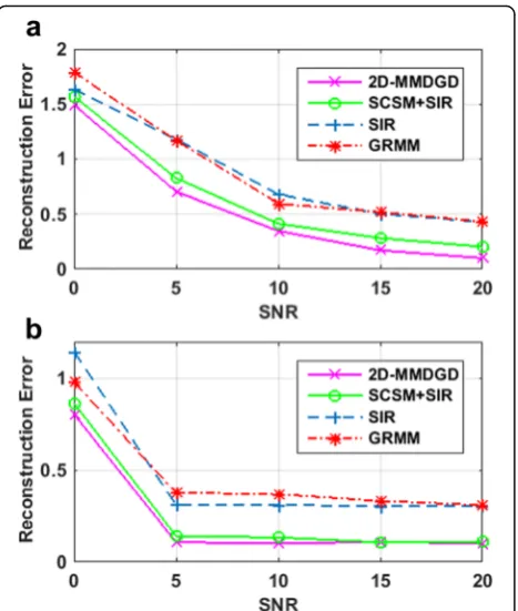
Fig. 6Comparison of reconstruction error for different methods versus the SNR in CS MIMO radar foraM= 4 andbM= 8
The reconstruction error versus the SNRs is shown in Fig. 6. As we see in Fig. 6a, the proposed method has bet-ter performance compared to other methods for small number of measurements in CS MIMO radar. Also, as depicted in Fig. 6b, our method and SCSM + SIR have nearly the same reconstruction error by increasing the number of measurements while outperforming SIR and GRMM methods.
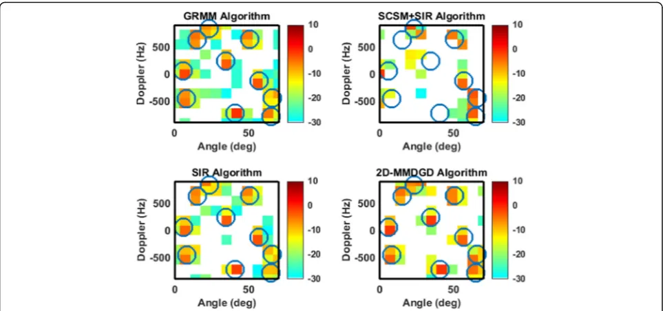
The second scenario that we considered is the one that the targets fall off the grid points. In this scenario, a ran-dom non-integer multiple of the angle resolution and a random non-integer multiple of the Doppler resolution are chosen as the angle and Doppler of each target. For simulation, we consider M= 4, Np= 5, Nd=Na= 11, Nr = 6 with a resolution of 7°.
The number of targets for Figs. 7 and 8 areNt= 4 and
Nt= 10, respectively. In these figures, the circles show the targets’ true locations and the estimated amplitudes are shown with color-coded rectangles in decibel. It is demonstrated that our proposed method are able to cap-ture the targets that fall off the grid points with lower sidelobes compared to other methods.
Figure 9 shows the runtime of measurement matrix design for different methods versus the number of mea-surements. The experiment is performed in MATLAB 8.1 environment using an Intel Core i7, 2.7 GHz proces-sor with 4 GB of memory, and under Microsoft windows 7 operating system. This figure demonstrates the effect-iveness of our proposed 2D method, and it shows clearly that the 2D-MMDGD has much lower computational
Fig. 9Comparison of runtime of measurement matrix design for different methods versus the number of measurements in CS MIMO radar
cost compared to the 1D one. Also, as explained in Sec-tion 5, SCSM + SIR has more runtime compared to our proposed 2D-MMDGD, and also the other methods.
7 Conclusions
We have introduced a new 1D and 2D CS model for a pulse-Doppler collocated MIMO radar. Then, we di-vided the measurement matrix design into four cases in which the measurement matrices applied to receivers and pulses can be equal or different. The measurement matrix design for all cases was proposed based on min-imizing MC of sensing matrix using gradient descent algorithm. Looking at the performance comparison be-tween 1D and 2D methods shows that case 3 can be the algorithm of choice for practical CS MIMO radar systems. The simulation results show that our proposed 2D-MMDGD, even in case 4 scenario outperform GRMM, SIR, and SCSM + SIR methods while having much lower computations.
8 Appendix 1
8.1 The statistical analysis of MC of sensing matrix A:
In this appendix, we analyze the MC of four cases from a statistical point of view. To do so, we obtain the mean and variance of MC for all cases and then compare their results. Let the components of measurement matrixφpm be considered as random variable.
The MC of A is proportional to μðAÞ∝ maxi≠jρi;j,
Since the statistical properties of measurement matrix φpm is independent of the number of pulses and antennas, and also it can be approximately inde-pendent of (i,j) as shown in [32], we can conclude that the mean and variance of δpm,ij for all cases are equal, i.e.,
Now, we analyze the variance of MC for all cases. Variance analysis of MC for case 1:
σ2
Variance analysis of MC for case 2:
σ2
σ2
Variance analysis of MC for case 4:
σ2
Consider the following Kroneker product properties [33]:
ifA=ΘT⊗B, thenai¼ ð ÞΘrd
Then, the MC ofAis obtained as,
μð Þ ¼A max
The authors would like to thank the Referees for the careful revision of the paper.
Authors’contributions
All the authors have contributed to the study conception and design of algorithms, theoretical analysis and simulations, drafting of manuscript, and critical revision. All authors read and approved the final manuscript.
Authors’information
Nafiseh Shahbazi received a B.S. degree in 2008 and an M.S. degree in 2008 in Electrical Engineering at Amirkabir University of Technology, Tehran, Iran. She is currently working for a Ph.D. degree in the School of Electrical and Computer Engineering, University of Tehran, from 2011. Her current research interests are in the areas of array signal processing, radar signal processing, and compressive sensing.
Aliazam Abbasfar received a B.Sc. (Highest Honors) and a M.Sc. degree in Electrical Engineering at the University of Tehran, Iran, in 1992 and 1995 and a Ph.D. degree in Electrical Engineering at the University of California Los Angeles (UCLA) in 2005. Between 2001 and 2004, he held a position as a senior design engineer in the areas of communication system design and digital VLSI/ASIC design with various start-up companies in California. Upon graduation from the UCLA, he joined Rambus Inc. where he was a Principal Engineer working on high-speed data communications on wireline serial and parallel links. He is currently an Assistant Professor at the University of Tehran. Mohammad Jabbarian-Jahromi received a Ph.D degree in Electrical Engineer-ing at Iran University of Science and Technology, Tehran, Iran, in 2016. His current research interests are in the areas of array signal processing, radar signal processing, and sparse reconstruction.
Competing interests
The authors declare that they have no competing interests.
Author details
1School of Electrical and Computer Engineering, University of Tehran, Tehran, Iran.2School of Electrical Engineering, Iran University of Science and Technology, Tehran, Iran.
Received: 27 August 2016 Accepted: 21 January 2017
References
1. DL Donoho, Compressed sensing. IEEE Trans Inf Theory52(4), 1289–1306 (2006)
3. M Mishali, Y Eldar, Blind multi-band signal reconstruction: compressed sensing for analog signals. IEEE Trans Signal Process.57(30), 993–1009 (2009)
4. J Ma, FX Le Dimet, Deblurring from highly incomplete measurements for remote sensing. IEEE Trans Geosci Remote Sens.47(3), 792–802 (2009) 5. SF Cotter, BD Rao, Sparse channel estimation via matching pursuit with
application to equalization. IEEE Trans Commun.50(3), 374–377 (2002) 6. J Trzasko, A Manduca, E Borisch, Highly under sampled magnetic resonance
image reconstruction via homotopic ell-0-minimization. IEEE Trans Med Imaging28(1), 106–121 (2009)
7. J Romberg, Imaging via compressive sampling (introduction to compressive sampling and recovery via convex programming). IEEE Signal Process Mag.
25(2), 14–20 (2008)
8. S Chen, D Donoho, M Saunders, Atomic decomposition by basis pursuit. SIAM J Sci Comput.20, 33–61 (1998)
9. R Baraniuk, P Steeghs, Compressive radar imaging, inProcess. Radar Conf, 2007, pp. 128–133
10. AC Gurbuz, JH McClellan, WR Scott, Compressive sensing for GPR imaging. in Proc. IEEE, 41st Asilomar Conf. Signals, Syst. Computer, Pacific Grove, CA, 2007, pp. 2223–2227.
11. M Herman, T Strohmer, Compressed sensing radar. in Proc. IEEE Int. Conf. IEEE, Acoustic Speech Signal Process., Las Vegas, NV, 2008, pp. 2617–2620 12. AC Gurbuz, JH McClellan, V Cevher, A compressive beamforming method.
in Proc. IEEE Int. Conf. Acoustic Speech Signal Process, Las Vegas, NV, 2008, pp. 2617-2620
13. AM Haimovich, RS Blum, LJ Cimini, MIMO radar with widely separated antennas. IEEE Signal Process Mag.25(1), 116–129 (2008)
14. P Stoica, J Li, MIMO radar with collocated antennas. IEEE Signal Process Mag.24(5), 106–114 (2007)
15. X Tan, W Roberts, J Li, P Stoica, Sparse learning via iterative minimization with application to MIMO radar imaging. IEEE Trans Signal Process.59(3), 1088–1101 (2011)
16. T Yardibi, J Li, P Stoica, M Xue, AB Baggeroer, Source localization and sensing: a nonparametric iterative adaptive approach based on weighted least squares. IEEE Trans Aerosp Electron Syst.46, 425–443 (2010) 17. M Jabbarian-Jahromi, MH Kahaei, Two-dimensional sparse solution for
bistatic MIMO radars in presence of jammers. 22nd Iranian Conference on Electrical Engineering (ICEE), pp. 1755–1759. IEEE, Tehran (2014) 18. Q Hou, Y Liu, Z Chen, Sh Su, Sparse radar imaging using 2D compressed
sensing. Proc. SPIE 9252, Millimetre Wave and Terahertz Sensors and Technology VII, Oct. 2014, 9252.
19. M Jabbarian-Jahromi, MH Kahaei, Two-dimensional iterative adaptive approach for a sparse matrix solution. IET Electron Lett50(1), 45–47 (2014) 20. A Ghaffari, M Babaie-Zadeh, C Jutten, Sparse decomposition of two
dimensional signals. in IEEE International Conf. on Acoustics, Speech and Signal Process., ICASSP 2009, pp. 3157–3160. IEEE, Taipei (2009) 21. HM Hyder, K Mahata, Range-Doppler imaging via sparse representation, in
IEEE Radar Conf. (RADAR), 2011, pp. 486–491
22. M Jabbarian-Jahromi, MH Kahaei, Two-dimensional SLIM with application to pulse Doppler MIMO radars. EURASIP J Adv Signal Process.69, 45–47 (2015) 23. M Jabbarian-Jahromi, MH Kahaei, Complex two-dimensional TNIPM for l1
norm-based sparse optimization to collocated MIMO radar. IEEJ Trans Electr Electron Eng.11(2), 228–235 (2016)
24. M Jabbarian-Jahromi, N Shahbazi, MH Kahaei, A Abbasfar, Fast two-dimensional sparse Bayesian learning with application to pulse Doppler multiple-input-multiple-output radars, inIET Radar, Sonar & Navigation, 2015, pp. 1–10 25. G Chen, D Li, J Zhang, Iterative gradient projection algorithm for
two-dimensional compressive sensing sparse image reconstruction. Elsevier Signal Process.104, 15–26 (2014)
26. Y Yu, AP Petropulu, HV Poor, MIMO radar using compressive sampling. IEEE J Selected Signal Process.4(1), 146–163 (2010)
27. T Strohmer, B Friedlander, Compressed sensing for MIMO radar—algorithms and performance. in Proc. IEEE, 43rdAsilomar Conf. Signals, Syst. Computer,
Pacific Grove, CA, 2009, pp. 464–468
28. DL Donoho, X Huo, Uncertainty principles and ideal atomic decomposition. IEEE Trans Inform Theory47(7), 2845–2862 (2001)
29. M Elad, Optimized projections for compressed sensing. IEEE Trans Signal Process.55(12), 5695–5702 (2007)
30. JM Duarte-Carvajalino, G Sapiro, Learning to sense sparse signals: simultaneous sensing matrix and sparsifying dictionary optimization. IEEE Trans Image Process.18(7), 1395–1408 (2009)
31. V Abolghasemi, S Ferdowsi, B Makkiabadi, S Sanei, On optimization of the measurement matrix for compressive sensing, inProcess. European Signal
Process. Conf, 2010, pp. 427–431
32. Y Yu, AP Petropulu, HV Poor, Measurement matrix design for compressive sensing-based MIMO radar. IEEE Trans Signal Process.59(11), 5338–5352 (2011)
33. A George, F Seber,A Matrix Handbook for Statisticians(Wiley, Hoboken, 2008)
34. JA Tropp, Greed is good: algorithmic results for sparse approximation. IEEE Trans Inf Theory50(10), 2231–2242 (2004)
35. S Boyd, L Vandenberghe,Convex Optimization(Cambridge University Press, Cambridge, 2004)
36. P Stocia, H He, J Li, New algorithms for designing unimodular sequences with good correlation properties. IEEE Trans Signal Process.57(4), 1415– 1425 (2009)
37. C Cartis, NIM Gould, PL Toint, On the complexity of steepest descent, Newton’s and regularized Newton’s methods for nonconvex unconstrained optimization. SIAM J Optim.20(6), 2833–2852 (2010)
38. C. D. Sa, K. Olukotun, and C., Global convergence of stochastic gradient descent for some non-convex matrix problems. Proceedings of the 32nd International Conference on Machine Learning (ICML-15), 2015.
Submit your manuscript to a
journal and benefi t from:
7Convenient online submission
7Rigorous peer review
7Immediate publication on acceptance
7Open access: articles freely available online 7High visibility within the fi eld
7Retaining the copyright to your article