! " #"# $ % %#
& ' ((( )
CSTuEPM: An Efficient Clustering Algorithm for Micro Array Gene Expression Data
Muhammad Rukunuddin Ghalib* VIT University, Vellore, India
D.K.Ghosh
Sri Nandanam College of Engg.and Tech, Tirupattur, India [email protected]
Abstract:Clustering analysis has been an important research topic in the machine learning field due to its wide applications in the area of data mining and bioinformatics. In recent years, it has even become a valuable and useful tool for in-silico analysis of microarray data. Although a number of clustering methods have been proposed, they are confronted with difficulties in meeting the requirements of automation, high cluster quality, and efficiency. An efficient clustering algorithm, namely, CSTuEPM (Correlation Search Technique using Euclidean proximity measure), which fits for analysis of gene expression data is proposed. The unique feature of this approach is that it incorporates the validation techniques into the clustering process so that high quality clustering results can be produced. The proposed work aims in incorporating Euclidean Proximity measure for measuring the similarity (or distance) between two data objects with ease.
Keywords:Data Mining, Cluster Analysis, Gene expression analysis, Micro Array Analysis
I. INTRODUCTION
Data mining refers to extracting or mining knowledge from large amounts of data. Alternatively, others view data mining as simply an essential step in the process of knowledge discovery. It is an essential process where intelligent methods are applied in order to extract data patterns. The data mining step may interact with the user or a knowledge base. The interesting patterns are presented to the user and may be stored as new knowledge in the knowledge base. Because of this data mining is the only one step in entire process, albeit an essential one because it uncovers hidden patterns for evaluation. From a data warehouse perspective, data mining can be viewed as an advanced stage on-line analytical processing (OLAP)[4], [8], [9], [10], [11], [12], [13]. Agrawal et al. (1993) describe three types of knowledge discovery: classification, associations and sequences. Classification attempts to divide the data into classes. A characterization of the classes can then be used to make predictions for new unclassified data. Classes can be a simple binary partition (such as “is-an-enzyme” or “not- an- enzyme”), or can be complex and many-valued such as the classes in our gene functional hierarchies. An overview of data mining and machine learning Associations are patterns in the data, frequently occurring sets of items that belong together. For example “pasta, minced beef and spaghetti sauce are frequently found together in shopping basket data”. Associations can be used to define association rules, which give probabilities of inferring certain data given other data, such as “if someone buys pasta and minced beef then there is a 75% likelihood they also buy spaghetti sauce”. Sequences are knowledge about data where time or some other ordering is involved, for example, to extract patterns from stock market data or gene sequence motifs. Although there are many data mining systems in the market, not all of them can perform true data mining. Data mining involves an integration of techniques from multiple disciplines such as database and data warehouse technology, statistics, machine learning, high-performance computing, pattern recognition, neural networks, data visualization, information retrieval,
image and signal processing and spatial or temporal data analysis
A. Cluster analysis
Unlike classification and prediction, which analyze class labelled data objects, clustering analyzes data objects without consulting a known class label. In general, the class labels are not present in the training data simply because they are not known to begin with. Clustering can be used to generate such labels. The objects are clustered or grouped based on the principle of maximizing the intraclass similarity and minimizing the interclass similarity. That is, clusters of objects are formed so that objects within a cluster have high similarity in comparison to one another, but are very dissimilar to objects in other clusters. Each cluster that is formed can be viewed as a class of objects, from which rules can be derived. Clustering can also facilitate taxonomy formation, that is, the organization of observations into a hierarchy of classes that group similar events together.
detection, where outliers (values that are far away from any cluster) may be more interesting than common cases. The following are typical requirements of clustering in data mining:
[a] Scalability
[b] Ability to deal with different types of attributes [c] Discovery of clusters with arbitrary shape
[d] Minimal requirement for domain knowledge to determine input parameters
[e] Ability to deal with noisy data
[f] Incremental clustering and insensitivity to the order of difficult to provide crisp categorization of clustering methods because these categorization may overlap, so that a method may have features from several categories. Nevertheless, it is useful to present a relatively organised picture of the different clustering methods which are as follows:
[a] Partitioning methods- k-Means and k-Medoids [b] Hierarchical methods- Agglomerative and divisive
Hierarchical clustering, BIRCH (balanced iterative reducing and clustering using hierarchies), ROCK, Chameleon.[2], [8], [9], [10], [11], [12], [13]
[c] Density based methods- DBSCAN, OPTICS, DENCLUE[9], [10], [12]
[d] Grid based methods- STING, WaveCluster[12], [13] [e] Model based clustering
methods-expectation-maximization, conceptual clustering, neural network approach- SOM(self organising feature maps)
[f] Clustering high dimensional data- CLIQUE, PROCLUS and pCluster[11]
[g] Constraint based cluster analysis[4], [8], [9], [10] [h] Outliers analysis[8], [12], [13]
B.1. Clustering Algorithms
As highlighted in the above section, gene expression matrix can be analyzed in two ways. For gene-based clustering [2], [7], genes are treated as data objects, while samples are considered as features.
B.2. Gene-based Clustering
The purpose of gene-based clustering is to group together co-expressed genes which indicate co- function and co-regulation. The K-means algorithm [2], [3], [4], [6] is a typical partition-based clustering method. Given a pre-specified number K, the algorithm partitions the data set into
K disjoint subsets which optimize the following objective distances of objects from their cluster centers. The K-means algorithm is simple and fast. The time complexity of K-means is O (l * k * n), where l is the number of iterations
and k is the number of clusters. However, it also has several drawbacks as a gene-based clustering algorithm. First, the number of gene clusters in a gene expression data set is usually unknown in advance. To detect the optimal number of clusters, users usually run the algorithms repeatedly with different values of k and compare the clustering results. The Self-Organizing Map (SOM) [2], [4], [5] was developed by Kohonen, on the basis of a single layered neural network. The data objects are presented at the input, and the output neurons are organized with a simple neighbour hood structure such as a two dimensional p * q grid. Each neuron of the neural network is associated with a reference vector, and each data point is “mapped” to the neuron with the “closest” reference vector. In the process of running the algorithm, each data object acts as a training sample which directs the movement of the reference vectors towards the denser areas of the input vector space, so that those reference vectors are trained to fit the distributions of the input data set. When the training is complete, clusters are identified by mapping all data points to the output neurons. One of the remarkable features of SOM is that it generates an intuitively-appealing map of a high-dimensional data set in 2D or 3D space and places similar clusters near each through the training process; hence, improperly-specified parameters will prevent the recovering of the natural cluster structure. Furthermore, if the data set is abundant with irrelevant data points, such as genes with invariant patterns, SOM will produce an output in which this type of data will populate the vast majority of clusters. In this case, SOM is not effective because most of the interesting patterns may be merged into only one or two clusters and cannot be identified.
B.3. Sample-based Clustering
Within a gene expression matrix, there are usually several particular macroscopic phenotypes of samples related to some diseases or drug effects, such as diseased samples, normal samples or drug treated samples. The goal of sample-based clustering is to find the phenotype structures or substructures of the samples. Previous studies have demonstrated that phenotypes of samples can be discriminated through only a small subset of genes whose expression levels strongly correlate with the class distinction. These genes are called informative genes [2]. The remaining genes in the gene expression matrix are irrelevant to the division of samples of interest and thus are regarded as noise in the data set. Thus, particular methods should be applied to identify informative genes and reduce gene dimensionality for clustering samples to detect their phenotypes. The existing methods of selecting informative genes to cluster samples fall into two major categories: supervised analysis
(clustering based on supervised informative gene selection) and unsupervised analysis (unsupervised clustering and informative gene selection).
a. Gene expression
mRNA and then translated into protein and those that are transcribed into RNA but not translated into protein (for e.g., tRNA and rRNAs).
b. CDNAs and ESTs
cDNA(complimentary DNAs) represent convenient ways of isolating and manipulating those portions of a Eukaryotic genome that are transcribed by RNA polymerase II. cDNAs are made from the RNA isolated from Eukaryotic cells. The resulting double stranded DNA copies of processed mRNAs can be cloned into vectors and maintained as a cDNA library.
ESTs (Expressed sequence tags)[1], [11], [14], [15]short sequence fragments(<200 base pairs) that are known to express collectively in a given tissue or pool of tissue. Clusters of these sub-fragments assemble into consensus sequences act as identifiers of genes or transcripts expressed in that tissue.
C. Proximity Measurement For Gene Expression Data
Proximity measurement measures the similarity (or distance) between two data objects. Gene expression data objects can be formalized as numerical vectors Oi = {oij | i j p}, where oij is the value of the jth feature for the ith data object and p is the number of features. The proximity between two objects measured by a proximity function of corresponding vectors Oi and Oj.
Euclidean distance [2], [4], [14], [15], [16]is one of the most commonly-used methods to measure the distance between two data objects. The distance between objects Oi and Oj in p-dimensional space is defined as:
2 interest than the individual magnitudes of each feature. Euclidean distance does not score well for shifting or scaled patterns (or profiles). To address this problem, each object vector is standardized with zero mean and variance one before calculating the distance. An alternate measure is Pearson’s correlation coefficient [2], which measures the similarity between the shapes of two expression patterns (profiles).
Given two data objects Oi and Oj, Pearson’s correlation coefficient is defined as,
respectively. Pearson’s correlation coefficient views each object as a random variable with p observations and measures the similarity between two objects by calculating the linear relationship between the distributions of the two corresponding random variables. Pearson’s correlation coefficient is widely used and has proven effective as a similarity measure for gene expression data. However, empirical study has shown that it is not robust with respect to outliers, thus potentially yielding false positives which assign a high similarity score to a pair of dissimilar patterns. If two patterns have a common peak or valley at a single feature, the correlation will be dominated by this feature,
although the patterns at the remaining features may be completely dissimilar. This observation evoked an improved measure called Jackknife correlation [2], where the Pearson’s correlation coefficient of data objects Oi and Oj in
equation 1.2 with the ith feature deleted. Use of the Jackknife correlation avoids the “dominance effect” of single outliers. More general versions of Jackknife correlation that are robust to more than one outlier can similarly be derived. However, the generalized Jackknife correlation, which would involve the enumeration of different combinations of features to be deleted, would be computationally costly and is rarely used. Another drawback of Pearson’s correlation coefficient is that it assumes an approximate Gaussian distribution of the points and may not be robust for non-Gaussian distributions. To address this, the Spearman’s rank-order correlation coefficient [2] has been suggested as the similarity measure. The ranking correlation is derived by replacing the numerical expression level oid with its rank rid among all conditions. However, as
a consequence of ranking, a significant amount of information present in the data is lost. Table Type Styles
II. RELATED WORK
A. k-means ALGORITHM
The K-means algorithm [2], [4], [6] is a typical partition-based clustering method. Given a pre-specified number K, the algorithm partitions the data set into K
disjoint subsets which optimize the following objective function: distances of objects from their cluster centers. The K-means algorithm is simple and fast. The time complexity of K-means is O (l * k * n), where l is the number of iterations and k is the number of clusters. However, it also has several drawbacks as a gene-based clustering algorithm. First, the number of gene clusters in a gene expression data set is usually unknown in advance. To detect the optimal number of clusters, users usually run the algorithms repeatedly with different values of k and compare the clustering results.
B. CST ALGORITHM
The CST algorithm [1] determines how to group the genes dynamically by utilizing Hubert’s statistic [1] during clustering without any user input parameter. It is precisely on such grounds that it can generate high quality clustering results automatically and efficiently. The experimental results show that the CST method can automatically produce the “nearly optimal” clustering result in much faster speed than other methods like k-means,
data set. The matrix S stores the degree of similarity between each pair of genes in the data set, with the degrees in range of [0, 1]. We can obtain the similarity by using any similarity measurements (e.g., Euclidean distance, Pearson’s correlation coefficient, etc.) according to the purposes of applications. Then, CST can automatically cluster the genes according to the similarity matrix S without any user-input parameters.
The main idea behind CST is to integrate the clustering method with the validation technique so that it can cluster the genes quickly and automatically. Moreover, based on the fact that biologists prefer quick obtaining of suboptimal results to long waiting for optimal results in real applications, CST aims at producing a “near-optimal” clustering result in fast speed. The validation index used here is Hubert’s statistic [1], [2] and its definition is as follows: Let X = [X (i,j)]and Y = [Y(i,j)] be two n x n proximity matrices on the same n genes.
From the viewpoint of correlation coefficient, X (i ,j) indicates the observed correlation coefficient of genes i and j, and Y(i ,j) is defined as follows:
1 if genes i and j areclustered in the same cluster
( , )
0 otherwise
Y i j
=
(1.5)The Hubert’s (gamma) statistic represents the point serial correlation between the matrices X and Y, and it is defined as follows when the two matrices are symmetric:
represents the better clustering quality. Therefore, the point serial correlation between the matrices X and Y can be used to measure the quality of clustering results. Since the where X (i,j)[0,1]. CST is a greedy algorithm that constructs clusters one at a time. The currently constructed cluster is denoted by Copen. Each cluster is started by a seed and constructed incrementally by adding (or removing) elements to (or from) Copen one at a time. The temporary clustering result of each addition (or removal) of x is computed by
CST takes turns between adding high positive correlation elements to Copen and removing high negative correlation elements from it. When Copen is stabilized by addition and removal procedure, this cluster is complete and the next one is started. The addition and removal procedures strengthen the quality of Copen gradually. Moreover, the removal procedure exterminates the cluster members that were inaccurately added at early clustering stages. In addition, a heuristics is added to CST for selecting an element with the maximum number of neighbours to start a new cluster.
III. PROPOSED ALGORITHM CSTUEPM
The pseudocode of CSTuEPM is shown in Figure.2.1 and Figure.2.2. The subroutine MaxValidaty(.) computes the possible maximum of measurement ’[1], yet, i.e., while a certain element is added (or removed). In the addition stage, it is equal to,
For the removal stage, it becomes:
Input: An n-by n- similarity matrix X 0. Initialization,
/* The collection of closed clusters*/
U={1,2,…,n}
/* Elements not yet assigned to any clusters*/
1.3 REMOVE: while MaxValidity()> max do Pick an element v bel Copenwith maximum
a(.)
Copen=Copen-{v}
/* Remove v from Copen*/ Sy = Sy- |Copen|
Sxy =Sxy -a(u)
For all i∈ U Copen Set a(i)=a(i)-X(u,i) /*Update the affinity*/ U=U U{v}
/* Insert v into U*/ max= MaxValidity()
1.4. Repeat steps ADD and REMOVE as long as there are no elements been removed
1.5. C=CU { Copen } end
2. Done, return the collection of cluster, C
Figure 2.2: The pseudocode of CSTuEPM
A. Features Used In The Proposed System
[a] Here an efficient clustering algorithm, namely, Correlation Search Technique using Euclidean proximity measure (CSTuEPM) is used.
[b] The unique feature is that it incorporates Euclidean Measure for Proximity measure of similarity between two data objects and results can be produced dynamically.
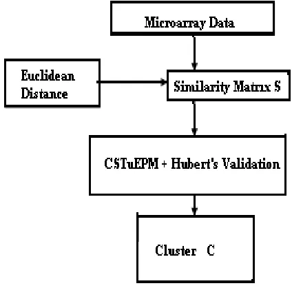
In the proposed system, Distance calculation used in the similarity matrix generation is Euclidean Distance proximity measure which is shown in Figure 1.
Figure 1: Overall Design of the Proposed System
B. Similarity Matrix Generation
Similarity matrix generation is done by computing the distances of sample genes in microarray Data set and accordingly to the resulted distance, the similarity matrix is formed. The overall steps of similarity matrix generation are shown in Figure 2 given below.
Micro array Data set
Compute d(i,j) = √( xi1-xj12+ xi2-xj22+…+ xip-xjp2)
If d(I,j)>=0 If d(i,j)=0 If d(i,j)=d(j,i) If d(i,j)<=d(i,h)+d(h,j)
Distance is non -veDistance is zero Distance is symmetric Triangular inequality
Similarity Matrix,S
Similarity Matrix Generation
Y Y Y Y
N N
N N
Figure 2: Algorithm for Similarity Matrix Generation
C. Steps In Cstuepm Algorithm
The following are the main steps in CST algorithm implementation.
[a] Similarity Matrix Generation [b] Initialization
[c] MaxValidity Calculation [d] Add Elements to Cluster
[e] Removing Elements From Cluster [f] Standardize Clusters
IV. IMPLEMENTATION
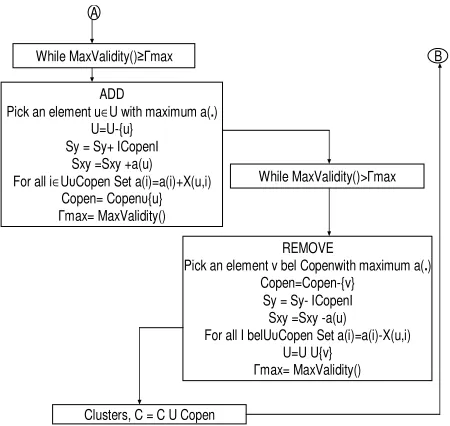
The following Figure 3 and Figure 4 show the overall implementation steps of CST algorithm.
Similarity matrix,X
Initialization, M=n (n-1)/2 n-1 n Sx= X(i, j)
i=1 j=i+1 Sy =0 Sxy =0
C=Ø U={1,2,…,n}
max=0
SEED:Pick an element u∈U with U=U-{u} For all i∈U Set a(i)=X(u,i)
Copen
Calculate MaxValidity() While( U Ø)
C=Ø a(.)=0
A
B
Clusters, C = C U Copen
REMOVE
Pick an element v bel Copenwith maximum a(.) Copen=Copen-{v}
Sy = Sy- Copen Sxy =Sxy -a(u) For all I belU Copen Set a(i)=a(i)-X(u,i)
U=U U{v} max= MaxValidity() While MaxValidity() max
ADD
Pick an element u∈U with maximum a(.) U=U-{u}
Sy = Sy+ Copen Sxy =Sxy +a(u) For all i∈U Copen Set a(i)=a(i)+X(u,i)
Copen= Copen {u} max= MaxValidity()
While MaxValidity()> max A
B
Figure 4: The CSTuEPM Algorithm (Contd…)
V. RESULTS AND DISCUSSION
Similarity Matrix Generation:
Similarity Matrix generation is done by taking some sample Datasets with the use of Euclidean Proximity measure. In the Euclidean Distance measure there are four different types of distances we get and accordingly the similarity matrix is generated.
For d(i,j) 0, Distance between the data object is non-negative.
For d(i,j) = 0, Distance between the data object is zero. For d(i,j) = d(j,i), Distance between the data object is symmetric.
For d(i,j) d(i,h) + d(h,,j), Distance between the data object triangular inequality.
Clustering Result on Data Set I (Cyanobacterium bacteria)
The dataset 1 consist of 919 rows and 75 columns gene expression data of Cyanobacterium bacteria. After the application of CAST algorithm the total number of clusters found is 22 with 5 outliers as shown in figure 5. When applied K-Means algorithm (K=10), the total number of clusters found are 10 with 0 outliers. Whereas 38 clusters are found when CSTuEPM algorithm is applied with 6 outliers as shown in figure 6.
Figure 5: Intensity image of clustering result of CAST on Data Set I
Figure 6: Intensity image of clustering result of CSTuEPM on Data Set I
Clustering Result on Data Set II (Cyanobaccilus baccilus)
The dataset II consist of 621 rows and 15 columns gene expression data of Cyanobaccilus baccilus. After the application of CAST algorithm the total number of clusters found is 14 with 3 outliers as shown in figure 7. When applied K-Means algorithm (K=10), the total number of clusters found are 10 with 0 outliers. Whereas 19 clusters are found when CSTuEPM algorithm is applied with 5 outliers as shown in figure 8.
Figure 7: Intensity image of clustering result of CSTuEPM on Data SetII
Figure 8: Intensity image of clustering result of CAST on Data Set II
Table 1: Experimental results on Data Set I
Methods Time(s) #Clusters Outliers Statisti
cs
CSTuEPM <1 38 6 0.917
CAST 25 22 5 0.900
k-means(k=10) 348 10 0 0.398
Table I: Experimental results on Data Set II
Methods Time(s) #Clusters Outliers Statistics
CSTuEPM <1 19 5 0.800
CAST 33 14 3 0.800
k-means(k=10) 412 10 0 0.375
We have results of various comparison of CSTeUPM to the existing clustering algorithms like CAST, K-Means performed on the available dataset-I and dataset-II in terms of time, number of clusters, outliers and validation
Figure 9: Comparison of CSTuEPM,CAST,K-Means on Dataset-I
0
Figure 10: Comparison of CSTuEPM,CAST,K-Means on Dataset-II
From the above tables and figures it is observed that CSTuEPM outperforms CAST and k-means substantially in both of execution time and clustering quality (Hubert’s Statistics). Moreover CSTuEPM also generates quite a number of clusters with small size which are mostly outliers. This means that CSTuEPM is superior to CAST and k-means in filtering out the outliers from the main clusters. Now we show the various time series plots of our datasets-I and datasets-II which is taken in terms of change in gene expression level in a range of durations like 0 minutes, 15 minutes, 1 hours, 6 hours and 15 hours respectively. This is illustrated in figures 11,12,13 and 14. Figure 15 shows the
Figure 11: Time series plot of change in gene expression level of Dataset-I
-6
Figure 13: Time series plot of change in gene expression level of Dataset-II
Figure 14: Time series plot of change in gene expression level of Dataset-I using CAST
Figure 15: Scatter plot of all the clusters of Dataset-I
another clusters with near perfection in the process of proximity measurement.Acknowledgment
VI. CONCLUSION AND FUTURE WORK
Clustering analysis is a very important task which suits for in-silico microarray gene expression data analysis in bioinformatics field. In this work Euclidean proximity measure is used for distance calculation in similarity matrix generation and reduced Hubert’s Statistics as validation technique which is an enhancement to the computation speed and its clustering quality of CST.
In future this work can be tested to more real microarray datasets and to system efficiency metrics like reduction of memory requirements. Data from microarray experiments on yeast were readily available on the internetbut tended to be noisy, and not as reliable as expected. We expect the quality and standardization of microarray experiments to improve in the near future.Many more sources of data become available as time goes on. Data about themetabolome will be the next challenge, and data about protein-protein interactions, pathways and gene networks will also need advanced clustering technologies. Many other genomes are now available, and their data also awaits mining.There is much still to be learned from the human genome, the genomes of plantsand animals and the many pathogenic organisms that cause disease..
VII. REFERENCES
[1] Vincent S. Tseng and Ching-Pin Kao, (2005)” Efficiently Mining Gene Expression Data via a Novel Parameterless Clustering Method”, IEEE/ACM TCBB, Vol.2.No.4, PP355-365.
[2] D. Jiang, C. Tang and A. Zhang, (2003)”Cluster Analysis for Gene Expression Data: A Survey”,dept. of CSE, State University of New York at Buffalo. [3] B. Sathiyabhama and N.P. Gopalan, (2006)”Mining
Gene Expression Data using Enhanced intelligence Clustering Technique”, WSEAS International Conferences Lisbon.
[4] Jiwai Han, Micheline Kamber, (2001)” Data Mininng Cocepts and Techniques.”, Elsevier Publication, 1st
Edition.
[5] T. Kohonen, “The Self-Organizing Map, (1990)” Proc. IEEE, vol. 78, no. 9, pp. 1464-1479.
[6] M.S. Aldenderfer and R.K. Blashfield, (1984) “Cluster Analysis” Beverly Hills, Calif.: Sage Publications. [7] Ben-Dor A., Shamir R. and Yakhini Z.
(1999)”Clustering gene expression patterns”. Journal of Computational Biology, 6(3/4):281–297.
[8] Bryan Bergeron, (2003) “Bioinformatics computing”, Prentice Hall of India Pvt. Ltd., New Delhi.
[9] Dan E. Krane and Michael L.Raymer, (2003) “Fundamental concepts of Bioinformatics”, Pearson Education Pvt. Ltd, New Delhi.
[10] S.Ignacimuthu, (2005) “Basic Bioinformatics”, Narosa publishing house, New Delhi.
[11] D.R. Westhead, J.H. Parish and R.M. Twyman, (2003) “Bioinformatics”, Viva Books Pvt. Ltd. New Delhi.
[12] Zoe Lacroix and Terence Critchlow, (2003)
“Bioinformatics managing scientific data”, Morgan Kauffman publishers.,Statistical Meetings of the American Statistical Association (Biometrics Section). [13] Brazma, Alvis and Vilo, Jaak. Minireview,
(2000)”Gene expression data analysis”. Federation of European Biochemical societies, 480:17–24.
[14] David R. Bickel. (2000) “Robust Cluster Analysis of
DNA Microarray Data: An Application of
Nonparametric Correlation Dissimilarity. “Proceedings of the Joint.
[15] Eisen, Michael B., Spellman, Paul T.,Brown, Patrick O.and Botstein David. (1998) “Cluster analysis and display of genome-wide expression patterns.” Proc. Natl. Acad. Sci. USA, 95(25)pp:14863–14868.