IJCSMC, Vol. 8, Issue. 9, September 2019, pg.01 – 10 A Comparative Study between Data Mining Classification and Ensemble Techniques for Predicting Survivability of Breast Cancer Patients

Available Online at www.ijcsmc.com

International Journal of Computer Science and Mobile Computing

A Monthly Journal of Computer Science and Information Technology

ISSN 2320–088X

IJCSMC, Vol. 8, Issue. 9, September 2019, pg.01 – 10

A Comparative Study between Data

Mining Classification and Ensemble

Techniques for Predicting Survivability

of Breast Cancer Patients

Dawngliani M.S

; Chandrasekaran N

; Samuel Lalmuanawma

¹Department of Computer Science, GZRSC, Aizawl, Mizoram, India

²Visiting Professor, Martin Luther Christian University, Former Director, CDAC, India ³Department of Management, Mizoram University, India

1

[email protected]; 2 [email protected]; 3 [email protected]

Abstract— Breast Cancer is the most common type of cancer prevalent among female cancer patients, while it also is the second most dreaded disease causing cancer death among women. A variety of data mining techniques, including Artificial Neural Networks (ANNs), Bayesian Networks (BNs), Support Vector Machines (SVMs) and Decision Trees (DTs) have widely been used in cancer research to facilitate the development of predictive models to create an effective decision making environment.

This study proposes a criteria for prediction of survivability of breast cancer patients, based on the analysis performed using four data mining classification techniques, which include, Decision Tree, Multilayer Perceptron, Naïve Bayes and Random Tree and comparing the results with those of four ensemble techniques such as Adaboost M1, Bagging, Voting and Stacking.

The dataset used in our experiment consists of 23 attributes containing 492 samples obtained from the Mizoram Cancer Institute of Aizawl, Mizoram, India. We are using data mining classifiers to predict the recurrence of breast cancer over a period of three years evaluated based on the comparison of their performance. Feature and attribute selections have been carried out to enhance the prediction accuracy of the computations.

Keywords— data mining, decision tree, neural network, support vector machine, naive bayes, support vector machine, ensemble method

I. INTRODUCTION

Breast cancer is a cancer that develops from breast tissue [1]. This cancer usually commences in the inner lining of milk ducts or the milk-producing glands (lobules). A malignant tumor implies that the cancer cells break out of the lobule where they began, with the potential to spread to lymph nodes and other areas of the body. Breast cancer that begins in the lobules is known as lobular carcinoma, while the one that develops from the ducts is called ductal carcinoma.

In Mizoram, the figure is close to that of Mumbai and stands at 26.6%. The table below shows the relative proportion of breast cancer in female in India (2007-2011)

TABLE I

FEMALE BREAST (ICD-10: C50)

Registry Total Number Relative % Rank

Mumbai 18528 5620 30.3 1

Bangalore 13125 2052 15.6 2

Chennai 17499 3921 22.4 2

Thiruvananthapuram 18809 5354 28.5 1

Dibrugarh 2276 336 14.8 1

Guwahati 4679 674 14.4 2

Chandigarh 2092 341 16.3 2

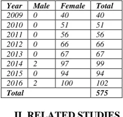
The numbers of breast cancer victims registered in Mizoram Cancer Institute are increasing each year in Mizoram and have shot up by more than 250% in the last 7 years alone. The table below lists the breast cancer statistics collected from Mizoram Cancer Institute during 2009-2016.

TABLE II

NUMBER OF BREAST CANCER VICTIMS REGISTERED IN MIZORAM CANCER INSTITUTE

Year Male Female Total

2009 0 40 40

2010 0 51 51

2011 0 56 56

2012 0 66 66

2013 0 67 67

2014 2 97 99

2015 0 94 94

2016 2 100 102

Total 575

II. RELATED STUDIES

An attempt is being made in this section to highlight and review some of the studies that have been carried out by various researchers working in the field of breast cancer, with the predictions being done using well known data mining techniques. Our current study utilizes a different technique as it employs a comparative study based approach to identify the most effective method appropriate for the predictive analysis.

Khodary, et al, 2018 [4] in their experiment used a 60 samples dataset obtained from the National Cancer Institute (NCI) of Egypt. The authors have attempted to develop a breast cancer prediction and diagnosis system based on the Rough Set (RS) theory.

Mohebian, et.al, 2017 [5] have reported developing a Hybrid Computer-aided-diagnosis System for Prediction of Breast Cancer Recurrence (HPBCR) using Optimized Ensemble Learning. Among 579 patients who participated in the study, 19.3% had recurrence of cancer five years after diagnosis. The authors employed a hybrid of three algorithms, viz., decision tree, SVM and MLP to conclude that they were able to obtain the best results using the hybrid approach.

Bazazeh & Shubair, 2017 [6] have compared the effectiveness of 3 data mining classifiers, viz., Support Vector Machine (SVM), Random Forest (RF) and Bayesian Networks (BN). The Wisconsin original breast cancer data set was used as a training set to evaluate and compare the performance of the three ML classifiers in terms of key parameters such as accuracy, recall, precision and area of ROC. They were able to establish that SVM performance was the best, in terms of accuracy, specificity, and precision. However, RF had the highest probability of correctly classifying tumors.

Guo, et al., 2017 [7] by their research were able to reveal certain determinant factors for early breast cancer recurrence by a decision tree based approach. The dataset contained information relating to 574 patients with non-metastatic invasive breast cancer, who received surgeries in the Leiden University Medical Centre containing 55 attributes. They excluded 71 dataset which had some missing values. They too applied a Decision Tree algorithm based on data relating to whether the patients develop early recurrence and on similarities of their clinical and pathological diagnoses. The classifier predicts whether a patient developed early disease recurrence, which was estimated to be about 70% accurate.

Suryachandra & Reddy, 2016 [8] in their paper compared 4 machine learning algorithms for breast cancer prediction. Random Forest and Naïve Bayes algorithms demonstrated a better ability to make predictions more accurately than Decision Tree and other algorithms even when the available information was scanty.

breast cancer survivability and recurrence. These algorithms were successfully applied to a novel breast cancer data set of the Clinical Centre of Kragujevac. The Naive Bayes classifier is selected as a model for prognosis of cancer survivability on the basis of 5 years survival rate, while the Artificial Neural Network algorithm exhibited best performance in the prognosis of cancer recurrence.

Tarek, et al, 2016 [10], in their work had developed and presented a new ensemble system for Cancer classification based on gene expression profiles. This approach had resulted in the development of a simple system that outperforms the ensemble system study suggested by Okun (2011). It also successfully addressed the three drawbacks, namely, enhancing result accuracy, covering more cancer types, and mitigating the effect of over-fitting. This work used K-NN classifier as a base member of the ensemble.

III. CLASSIFICATION TECHNIQUE USED IN THE CURRENT WORK

Data Mining as it relates to computer science, is the process of discovering interesting and useful patterns and relationships that exist in large amounts of data. This field combines several tools and artificial intelligence with database management systems to analyze large digital collections known as datasets [11]. Data mining can be considered as the heart of the Knowledge Discovery Database process. This is the area, which deals with the use of a number of machine learning algorithms to obtain useful patterns from the datasets.

Although there are a number of data mining algorithms and tools available we will mainly be considering the following four data mining classifiers and four ensemble methods.

A. Decision Tree

The core algorithm for building decision trees called ID3 was formulated by J. R. Quinlan which employs a top-down, greedy search through the space of possible branches with no backtracking. This technique is commonly applied for gaining information for the purpose of decision-making when (if...else) type of conditional rule becomes applicable and it usually starts with a root node, see Fig. below. This is a typical example, say for a Bank to use to determine whether a customer can be extended a loan [12]. The most common decision tree algorithms are J48, ID3, C4.5, and CART. In this study, in the current study, J48 algorithm has been used to analyze the performance with and without feature selection techniques.

Fig. 1 Example of decision tree [12]

B. Support Vector Machine

Support vector machine (SVM) is a supervised machine learning algorithm, which is mostly used for solving classification problems. Depending upon the number of features of the dataset, each data is plotted on those many number of dimensional space [13]. Classification analysis is then performed to determine the hyper-plane to isolate the dataset associated with two different classes and to increase the lower margin that connects the hyperplane with each individual data class in the Euclidean space, even if the data are not breakable [14]. The purpose of the increment is to select the most powerful hyperplane. If the data are not breakable, it tries to keep the total error, i.e., the distance from the hyperplane to the incorrectly classified data record, below a certain user-defined threshold. In the current study, we have employed SMO classifier under support vector machine.

C. Neural Network

ability to capture the complex and nonlinear interaction between prognostic markers and the predicted outcome. In our current study, the Multilayer Perceptron (MLP) algorithm has been employed to compare the accuracy and performance with and without feature selection techniques.

D. Bayesian networks

The Bayesian networks belong to the probabilistic graphical model family, in which each edge corresponds to a conditional dependency, and each node corresponds to a unique random variable. In other words, nodes in the graph represent random variables, and the edges represent the probabilistic dependencies between random variables. They are given as either a table or conditional probability function.

A Bayesian Network consists of a directed acyclic graph (DAG) that represents causal relationships between arbitrary variables and parameters. Combining both graphical structure and conditional probability confers full power to the model. They are frequently used in bioinformatics for the task of integrating various gene prediction systems. They allow finding the closest corresponding network to the existing training set of independent parameters. This process can be obtained based on statistical function which finds the optimal network by evaluating each network with consideration to the training dataset [14]. One of the most popular Bayesian networks called Naive Bayes is employed in this study.

E. Ensemble method

Ensemble algorithms are a powerful class of machine learning algorithms that combine the predictions from multiple models to determine the most optimal one [15]. We have used four ensemble methods for our current study and their salient features are explained below:

1. Boosting: Boosting is an ensemble machine learning algorithm typically used for tackling classification problems. We have used AdaBoost M1, a boosting model, which has successfully been implemented to increase the accuracy of the model. AdaBoost uses short decision tree models, normally referred to as decision stumps, each with a single decision point. Each instance in the training dataset is weighed and the weights are updated based on the overall accuracy of the model and whether an instance was classified correctly or not. Subsequent models are trained and added until a minimum accuracy is achieved or no further improvements are possible. Each model is weighted based on its skill and these weights are used when combining the predictions from all of the models on new data [16].

2. Bagging: The full form of bagging is Bootstrap Aggregation. It an ensemble algorithm that can be used for classification as well as regression. Bagging is a statistical estimation technique where a statistical quantity like a mean is estimated from multiple random samples of the dataset (with replacement). It is a useful technique when only a limited amount of data is available and one is interested in obtaining a more robust estimate of a statistical quantity. Multiple random samples of the training dataset are drawn with replacement and used to train multiple machine learning models or algorithms. Each model is then used to make a prediction and the results are averaged to give a more robust prediction. It is a technique that is best used with models that have low bias and high variance, meaning that the predictions they make are highly dependent on the specific data from which they were trained. The most used algorithm for bagging that fits this requirement of high variance is decision trees [16].

3. Voting: Voting is the simplest ensemble algorithm, and is often very effective for solving classification or regression problems. Voting works by creating two or more sub-models, with each one of sub-models making predictions. The sub-models are combined in some way that, by taking the mean or the mode of the predictions. Each sub-model can vote to determine the eventual outcome [17]. In this study, we have done voting with four classifiers such as J48, Naive Bayes, MLP and SMO.

4. Stacking: Stacked Generalization or Stacking is a simple extension to Voting that can also be used to solve classification and regression problems. In addition to selecting multiple sub-models, stacking allows specifying another model to learn how best to combine the predictions from the sub-models. The latter is also known as meta-classifier. Because a meta-classifier is used to best combine the predictions of sub-models, this technique is sometimes called blending, which implies that predictions can be blended together [17]. In this study, we have done stacking with four classifiers such as J48, Naive Bayes, MLP and SMO. For our work, J48 has been used as a meta classifier.

IV. METHODOLOGY

Knowledge discovery process implies extracting useful relationships and patterns from large databases [18]. This necessitates the creation of a systematic method. It is pertinent to state that quality data is essential to secure accurate and useful outcomes. Vague data is a common term in data mining that describes some unwanted data characteristics such as incompleteness, noisy, and inconsistency.

The following five steps have carefully be undertaken during the research: 1. Data Collection

4. Analyze using Data Mining methods 5. Evaluation & Testing

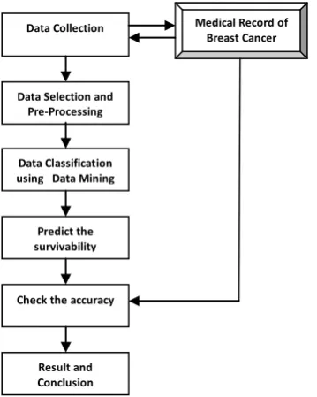
Fig. 2: Data Mining Methodology

A. Data collection

Breast Cancer Data was collected from Mizoram Cancer Institute from 2009 till 2016. The collected data contain 25 attributes from the medical record which has been obtained in HBCR (Hospital Based Cancer Registry) format. The format ensures that the datasets have records of Registration No., Hospital Registration No,, Date of Diagnosis, Age (in years), Date of Birth, Sex, Height, Weight, Contact, Method of Diagnosis, Laterality, Morphology, Sequence, Socio-Economic Status, Co-Morbid Condition, Tumour Size, Axillary Lymph Node, Supraclavicle Node, Skin Involvement, TNM Stage, Stage Grouping, Type of prior Treatment given, Habitual Data, Vital Status and Disease Status. Some of the entries were incomplete implying that those records have to be discarded before processing. Moreover, those attributes that have been found to be redundant or not relevant have to be excluded from the analysis. It was, hence, determined to be prudent to consider these attributes for the analysis, viz., Age (in years), Sex, height, weight, Laterality, Morphology, Socio-Economic Status, Co-Morbid Condition, Axillary Lymph Node, Skin Involvement, Stage Grouping, Usage of cigarette, tobacco, alcohol, pan masala, betelnut and recurrence. A total of 492 data record fell into this group.

B. Data selection

Data selection or feature selection is extensively used, which is an area of active research interest pertaining to pattern recognition, statistics, and data mining in the medical domain. Feature selection invariably involves reducing the number of attributes to improve the accuracy of the outcome. The attributes are reduced by removing irrelevant and redundant attributes, which do not have much importance in determining the outcome. The aim behind feature selection is to select a subset of records of variables by ignoring features with little or less important information. Less important data can be determined by using the evaluator in WEKA (Waikato Environment for Knowledge Analysis), which is an open-source free machine learning software package [19]. It contains tools for performing collection preprocessing, classification, clustering, association and visualization, together with an attractive graphical user interfaces. The feature selection improves the performance of the classification techniques [20]. The feature selection evaluator that we selected include, CfsSubsetEval, ChisquaredAttributeEval, InfogainAttributeEval and GainRationAttribEval. CfsSubsetEval to evaluate the worth of a subset of attributes by considering the individual predictive ability of each feature and select those attributes which are useful in prediction of accuracy [21]. ChiSquaredAttributeEval evaluates the worth of an attribute by computing the value of the chi-squared statistic with respect to the class [21]. InfoGainAttributeEval evaluates the worth of an attribute by measuring the information gain with respect to the class [21]. GainRatioAttributeEval evaluates the worth of an attribute by measuring the gain ratio with respect to the class [21]. The evaluator checks each subset using ranker method and ranks them according to their significance and relevance. The subset with a rank lower than the threshold will be excluded.

Data Collection Medical Record of Breast Cancer

Patients Data Selection and

Pre-Processing Data Classification using Data Mining

Techniques Predict the survivability Check the accuracy

C. Data pre-processing

Completeness, accuracy, and consistency of the data are factors that define data quality. Data preprocessing is an important step in data mining process to satisfy data quality requirements. Therefore, the current research is to utilize data pre-processing tasks to ensure the dataset is ready for mining process in order to produce accurate results. Hence, it has to be emphasised that for the data to be analyzed quantitatively, the collected attributes should be coded in numbers sometimes, ranging from 1 to 10. This necessitates allocation of numbers when the data is entered in text (non numeric) form, based on the order it follows, At the end of this exercise, the data should be ready for data mining analysis.

D. Analyze using data mining methods

A model is to be proposed and tested for its accuracy using WEKA. WEKA provides the environment to calculate the information gain and contains some data mining and machine learning methods for data pre-processing, classification, regression, clustering, association rules, and visualization [19].

Using WEKA, the Breast Cancer dataset was analyzed by data mining classifiers. In this study, we have used four classifiers such as J48, Naive Bayes, MLP, SMO and four ensemble classifiers such as Adaboost M1, Bagging, Vote and Stacking. Results are interpreted in the form of tables and charts.

E. Evaluation and Testing

In order to evaluate our results, we are using a 10 fold cross-validation and ROC curve. Cross-validation is a technique to evaluate predictive models by partitioning the dataset into a training set to train the model, and a test set to evaluate it [22]. In 10-fold cross-validation, the original sample is randomly partitioned into 10 equal sized subsamples. Of the 10 subsamples, a single subsample is retained as the testing data, and the remaining 9 subsamples are used as training data. It is repeated 10 times, with each of the 10 subsamples used exactly once as the testing or validation data. The results from each fold can then be averaged to produce a single estimation.

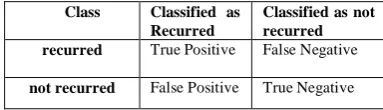
The receiver operating characteristic curve is used to check or visualize the performance of classifiers at various thresholds settings. It shows how much a classifier is capable of distinguishing between classes. Higher the AUC, the better the model is at predicting true as true and false as false [23]. The ROC curve is plotted with a true positive rate against the false-positive rate where true positive rate is on the y-axis and the false positive rate is on the x-axis. The resulting analysis builds a confusion matrix as follows:

TABLE III CONFUSION MATRIX

Class Classified as Recurred

Classified as not recurred recurred True Positive False Negative

not recurred False Positive True Negative

The sensitivity, specificity and accuracy are calculated as follows: Sensitivity (true positive rate) = TP/ (TP+FN)

Specificity (true negative rate) = TN/ (FP+TN) Accuracy = (TP+TN)/ (TP+FP+TN+FN)

Where TP is true positive, TN is true negative, FP is false positive and FN is a false negative. From the sensitivity, specificity, and accuracy, the most efficient algorithm can be found.

V. EXPERIMENTAL RESULT

In this paper, we are using feature selection using four evaluators namely CfsSubsetEval, ChisquaredEval, InfogainAttributeEval and GainRationAttribEval. The first evaluator chooses only five attributes while the rest reject only two attributes (i.e we have 21 attributes for classification). The table below shows the result with and without feature selection. Features such as age and BMI is excluded in the attribute feature selection (which is the result of the three evaluators viz ChisquaredEval, InfogainAttributeEval, and GainRationAttribEval).

TABLE IV

PERFORMANCE ANALYSIS OF CLASSIFIERS WITH AND WITHOUT FEATURE SELECTION IN TERMS OF ACCURACY.

Sl No

Classifier Without Feature Selection

Feature Selection

(without age/BMI) Average

1 J48 84.2105 83.8596 84.0351

3 MLP 75.7895 79.2982 77.5439

4 SMO 81.4035 81.4035 81.4035

5 Adaboost M1 82.8070 82.8070 82.8070

6 Bagging 83.5088 82.4561 82.9825

7 Voting 83.1579 83.8596 83.5088

8 Stacking 81.4035 81.0526 81.2281

Average 81.00878 81.62279

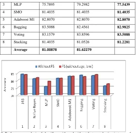
Fig. 3: Performance analysis of classifiers with and without feature selection in terms of accuracy.

From the average, the feature selection gives a higher accuracy (82.2514%) compared to the selection done without feature selection (81.4620%). Also, we see that decision tree J48 has the highest accuracy of 84.2105%, followed by Voting (83.5088%) and Bagging (82.9825%) which are both ensemble models. The chart below shows the comparison between classifiers performed with and without feature selection.

As already mentioned, we have used four evaluators for feature selection. The first evaluator chooses only five (5) attributes while the rest chose 21 attributes. These evaluators rank each attribute depending on their contribution toward classification. Now we are going to select the top 10 and top 15 attributes depending upon the rank of the attribute which was given by the evaluator to check for its accuracy performance.

TABLE V

COMPARISON OF VARIOUS CLASSIFIERS WITH DIFFERENT EVALUATORS.

S l N o C la ss ifi e r w ith o u t fe a tu r e se le c ti o n w ith F S w ith o u t a g e /b m i c fs e v a l C h i sq u a r e to p 1 0 C h i sq u a r e to p 1 5 in fo g a in to p

10 info

g

a

in

to

p

15 ga

in r a ti o to p 1 0 g a in r a ti o n to p 1 5 A v e r a g e

1 J48 84.2105 83.8596 83.8596 82.8070 84.2105 83.5088 84.2105 83.1579 84.2105 83.7817

2 Naïve Bayes

81.0526 81.7544 83.1579 82.4561 83.1579 82.8070 82.1053 82.4561 82.1053 82.3392

3 MLP 75.7895 79.2982 83.5088 75.7895 77.1930 75.7895 72.9825 77.1930 74.3860 76.8811

4 SMO 81.4035 81.4035 79.6491 78.9474 80.0000 79.2982 80.0000 78.5965 80.3509 79.9610

5 Adaboost M1

82.8070 82.8070 82.8070 81.7544 82.8070 81.7544 82.8070 82.8070 82.8670 82.5798

6 Bagging 83.5088 82.4561 81.7544 82.4561 82.4561 82.4561 82.4561 82.8070 82.4561 82.5341

7 Voting 83.1579 83.8596 82.4561 81.4035 81.4035 80.3509 81.7544 81.0526 81.0526 81.8323

8 Stacking 81.4035 81.0526 82.4561 82.4561 81.0526 83.5088 80.3509 82.4561 80.0000 81.6374

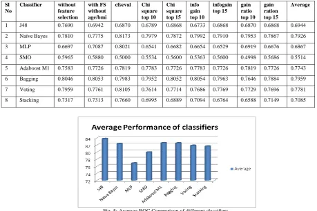
Fig. 4: Average performance of each classifier using different evaluators.

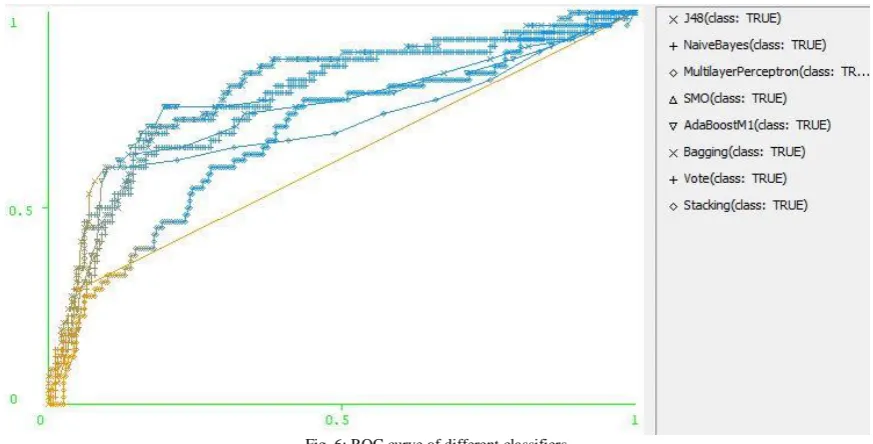
In the next step, an attempt has been made to evaluate each classifier in terms of ROC (Receiver Operating Characteristics). Table VI shows the ROC value of each classifier. The top three classifiers in terms of ROC value are Bagging 90.7959), Naïve Bayes (0.7926) and Voting (0.7781). This implies that ensembled classifiers are more efficient when compared to ordinary classifiers. Figure 5 shows the average ROC comparison of different classifiers and Figure 6 shows the pictorial representation of ROC curve of different classifiers.

TABLE VI

ROC COMPARISON OF DIFFERENT CLASSIFIERS.

Sl No

Classifier without feature selection

with FS without age/bmi

cfseval Chi square top 10

Chi square top 15

info gain top 10

infogain top 15

gain ratio top 10

gain ration top 15

Average

1 J48 0.7690 0.6942 0.6870 0.6789 0.6868 0.6733 0.6868 0.6870 0.6868 0.6944

2 Naïve Bayes 0.7810 0.7775 0.8173 0.7979 0.7872 0.7992 0.7910 0.7953 0.7867 0.7926

3 MLP 0.6697 0.7087 0.8021 0.6541 0.6682 0.6654 0.6529 0.6919 0.6676 0.6867

4 SMO 0.5965 0.5880 0.5000 0.5534 0.5600 0.5363 0.5600 0.4998 0.5686 0.5514

5 Adaboost M1 0.7583 0.7726 0.7819 0.7783 0.7726 0.7783 0.7726 0.7819 0.7726 0.7743

6 Bagging 0.8046 0.8053 0.7983 0.7952 0.8052 0.8054 0.7963 0.7646 0.7884 0.7959

7 Voting 0.7959 0.7761 0.8105 0.7614 0.7714 0.7686 0.7769 0.7729 0.7696 0.7781

8 Stacking 0.7317 0.7313 0.7660 0.6995 0.6889 0.7094 0.6764 0.6588 0.7149 0.7085

Fig. 6: ROC curve of different classifiers

VI. CONCLUSION

In this research, we have endeavoured to compare four classifiers with ensemble methods to evaluate the percentage accuracy for predicting breast cancer recurrence. The medical data has been obtained from Mizoram Cancer Institute, Aizawl, North East India. J48 shows the highest accuracy when averaging different evaluators. In terms of ROC, Voting (which is an ensemble method consisting of J48, Naïve Bayes, MLP and SMO) is found to be the most efficient method. By taking the average, performance accuracy of ordinary classifiers has been determined to be 80.7407%, while that of ensemble classifier is 82.1459%. Similarly, ROC value of ordinary of ordinary classifier computed from this work is 0.6813 and that of ensemble classifier is 0.7642. Hence, we can conclude that the overall performance of ensemble classifier far exceeds that of the conventional classifier by a significant margin.

ACKNOWLEDGEMENT

We would like to thank Dr. Jerry Lalrinsanga, Medical Oncologist of Mizoram Cancer Institute (MCI), Aizawl, for supporting this research work by giving us permission to collect breast cancer datasets from MCI. The authors express their sincere gratitude to MLCU for facilitating and extending all possible help to complete this particular research work.

REFERENCES

[1] NCI, “Breast Cancer,” vol. 2020, no. March 2019. 2014.

[2] World Cancer Research Fund and American Institute for Cancer Research, “Breast cancer statistics | World Cancer Research Fund,” Cancer Trends. 2018.

[3] N. Report, “FEMALE BREAST ( ICD-10 : C50 ),” pp. 120–125, 2011.

[4] S. Khodary, M. Hamouda, M. E. Wahed, R. H. Abo, and K. Riad, “Computer Methods and Programs in Biomedicine Robust breast cancer prediction system based on rough set theory at National Cancer Institute of Egypt,” Comput. Methods Programs Biomed., vol. 153, pp. 259–268, 2018.

[5] M. R. Mohebian, H. R. Marateb, M. Mansourian, M. Angel, and F. Mokarian, “A Hybrid Computer-aided-diagnosis System for Prediction of Breast Cancer Recurrence ( HPBCR ) Using Optimized Ensemble Learning,” Comput. Struct. Biotechnol. J., vol. 15, pp. 75–85, 2017.

[6] D. Bazazeh and R. Shubair, “Comparative study of machine learning algorithms for breast cancer detection and diagnosis,” Int. Conf. Electron. Devices, Syst. Appl., pp. 2–5, 2017.

[7] J. Guo et al., “Revealing determinant factors for early breast cancer recurrence by decision tree,” Inf. Syst. Front., vol. 19, no. 6, pp. 1233–1241, 2017.

[8] P. Suryachandra and P. V. S. Reddy, “Comparison of machine learning algorithms for breast cancer,” Proc. Int. Conf. Inven. Comput. Technol. ICICT 2016, vol. 2016, 2016.

[10] S. Tarek, R. A. Elwahab, and M. Shoman, “Gene expression-based cancer classification,” Egypt. Informatics J., 2016.

[11] C. Clifton, “Definition of Data Mining,” Encyclopaedia Britannica, 2014. [Online]. Available: www.britannica.com.

[12] T. Plapinger, “What is a Decision Tree?”, https://towardsdatascience.com/what-is-a-decision-tree-22975f00f3e1, 2017.

[13] S. Ray, “Understanding Support Vector Machine algorithm from examples (along with code)”, 2017, https://www.analyticsvidhya.com/blog/2017/09/understaing-support-vector-machine-example-code/

[14] A. K. Pujari, “Data Mining Techniques”, Third edit. University Press Private Limited, 2013.

[15] E. Lutin, “Ensemble Methods in Machine Learning: What are They and Why Use Them?,” Medium: Towards Data Science. 2017.

[16] D. Opitz and R. Maclin, “[Opitz99] Popular ensemble methods_an empirical study.pdf,” vol. 11, pp. 169– 198, 1999.

[17] R. Polikar, “(Ensemble Learning).” 2008.

[18] W. J. Frawley, G. Piatetsky-Shapiro, and C. J. Matheus, “Knowledge Discovery in Databases : An Overview,” vol. 13, no. 3, pp. 57–70, 1992.

[19] I. H. Witten, E. Frank, and M. A. Hall, Data Mining: Practical Machine Learning Tools and Techniques, Third Edit. Morgan Kaufmann, San Francisco, 2011.

[20] A. Lebbe, S. Saabith, E. Sundararajan, and A. A. Bakar, “Comparative Study on Different Classification Techniques for Breast Cancer Dataset,” Int. J. Comput. Sci. Mob. Comput., vol. 3, no. 10, pp. 185–191, 2014.

[21] Weka Machine Learning Project, http://www.cs.waikato.ac.nz/~ml/index.html.

[22] F. Wikipedia, “Cross-validation (statistics) - Wikipedia.” 2019, https://en.wikipedia.org/wiki/Cross-validation_(statistics).