Western University Western University
Scholarship@Western
Scholarship@Western
Electronic Thesis and Dissertation Repository
4-23-2018 1:15 PM
A Framework for Modelling User Activity Preferences
A Framework for Modelling User Activity Preferences
Roberto Barboza Junior
The University of Western Ontario
Supervisor
Miriam A.M. Capretz
The University of Western Ontario
Graduate Program in Electrical and Computer Engineering
A thesis submitted in partial fulfillment of the requirements for the degree in Master of Engineering Science
© Roberto Barboza Junior 2018
Follow this and additional works at: https://ir.lib.uwo.ca/etd
Part of the Software Engineering Commons
Recommended Citation Recommended Citation
Barboza Junior, Roberto, "A Framework for Modelling User Activity Preferences" (2018). Electronic Thesis and Dissertation Repository. 5332.
https://ir.lib.uwo.ca/etd/5332
This Dissertation/Thesis is brought to you for free and open access by Scholarship@Western. It has been accepted for inclusion in Electronic Thesis and Dissertation Repository by an authorized administrator of
The availability of location data increases every day and brings the opportunity to mine these
data and extract valuable knowledge about human behaviour. More specifically, these data may
contain information about users’ activities, which can enable, for example, services to improve
advertising campaigns or enhance the user experience of a mobile application. However,
sev-eral techniques ignore the fact that users’ context other than location and time, such as weather
conditions, influences their behaviour. Moreover, several studies focus only on a single data
source, addressing either data collected without any type of user interaction, such as GPS data,
or data spontaneously shared by the user, for instance, from location-based social networks
(LBSNs), but not both.
This thesis proposes a framework that aims to predict users’ current activity preferences
(UCAP). UCAP handles data gathered from different sources. It takes into account users’
historical data, their current context, and other external contexts such as weather conditions.
The framework was evaluated on five real-world datasets. The results demonstrated the
accuracy of the proposed solution, which was on average 12.3% more accurate than a
state-of-the-art technique. Moreover, the experiments evaluated the impact of the main components on
the prediction results and showed that UCAP is not constrained by dataset size.
Keywords: Location-Based Services, Location-Based Social Networks, Location-Data
Preprocessing, Context Aware, User Behaviour Prediction, Location-Based User Clustering
Acknowlegements
First, I would like to thank my supervisor Dr. Miriam Capretz. Dr. Capretz believed in my
potential and gave me the opportunity to study under her guidance. Without her support, this
thesis would not become a reality. Thank you for your patience, time and effort to make this
whole experience possible.
I will never truly be able to express how thankful I am to my father, Roberto Barboza, and
my mother, Cecilia Leite de Araujo Barboza, for being there whenever I needed it, and even
when I thought I did not need it. Thank you for helping me find my own way. I would never
have made it this far without you. I love you both. I would also like to extend my heartfelt
appreciation to my brother Vinicius, who is always willing to talk with me about anything and
supporting me no matter what. I am blessed to be a part of this family.
I would not be here without the support of my wife, Andrea Okuda, who left everything
behind to join me in this challenge. You have inspired me to strive to be the best version of
myself. Thank you for being with me. Love you.
My sincere thanks must also go to my former and current laboratory colleagues and friends:
Wander Queiroz, Alex L’Heureux, Will Aguiar, Jos´e Miguel Alves, Rafael Aguiar, Daniel
Berhane Araya, Dr. Wilson Higashino, Dr. Katarina Grolinger and Dr. Ahmed Eltahawi, who
helped throughout this research. Special thanks to Dr. Hany ElYamany and Dr. Mahmoud
ElGayyar for lending me their expertise to my research, spending countless hours reviewing
my work, and for believing in my work even when I had questions about it. Thank you.
I cannot forget my old-time friends, Mauro Ribeiro and Dennis Bachmann, who did
every-thing in their power to assist me since I decided to come to Canada. Thanks for being nearby
and for all the discussions about life, the universe and everything.
Last but not least, thanks to my family, my friends, and all my colleagues who accompanied
me during life, and for all of those that will never forgive me for not mentioning them here.
Abstract i
Acknowlegements ii
List of Figures vi
List of Tables vii
1 Introduction 1
1.1 Motivation . . . 1
1.2 Contribution . . . 3
1.3 Organization of the Thesis . . . 4
2 Background and Literature Review 6 2.1 Background . . . 6
2.1.1 Data Preprocessing . . . 6
2.1.2 Machine Learning . . . 10
2.2 Literature Review . . . 13
2.3 Summary . . . 18
3 UCAP Framework 19 3.1 Preprocessing Layer . . . 19
3.1.1 Events Merger . . . 22
3.1.2 Inactive Users Filter . . . 24
3.1.3 Context Merger . . . 25
3.1.4 Data Splitter . . . 25
3.2 Feature Engineering Layer . . . 26
3.2.1 Clusterer Feature Extractor . . . 26
3.2.2 Clusterer . . . 28
3.2.3 Feature Enhancer . . . 29
3.3 Prediction Layer . . . 30
3.3.1 Prediction Engine . . . 31
3.3.2 Evaluator . . . 31
3.3.3 Tuner . . . 32
3.4 Presentation Layer . . . 32
3.4.1 Storage . . . 34
3.4.2 Model Handler . . . 34
3.5 Summary . . . 35
4 Case Studies 36 4.1 Implementation and Experiments . . . 36
4.1.1 Data Analysis . . . 38
4.1.2 Experiment 1: Impact of the UCAP Components . . . 39
4.1.3 Experiment 2: Comparison with a Different Approach . . . 44
4.1.4 Experiment 3: Comparison between Different Datasets . . . 45
4.2 Discussion . . . 46
4.3 Summary . . . 48
5 Conclusions and Future Work 49 5.1 Conclusions . . . 49
5.2 Future Work . . . 50
Bibliography 52
List of Figures
1.1 A scenario showing a user and two different locations. . . 3
2.1 Data Preprocessing Categories . . . 7
3.1 Data flow of the UCAP Framework . . . 20
3.2 UCAP inputs example. . . 21
3.3 User Events dataset before and after the Events Merger . . . 23
3.4 Example of: (a) External Context dataset; (b) Context Merger being performed 25 3.5 Tuning process flow. . . 33
4.1 Probability distribution of the events per user . . . 40
4.2 Number of events along time . . . 41
4.3 Number of activities per event . . . 42
4.4 UCAP variations prediction results . . . 44
4.5 UCAP andSTAPcomparison . . . 45
4.6 UCAP prediction results on different datasets . . . 47
3.1 Features with domain . . . 30
4.1 XGBoost Parameters . . . 37
4.2 Datasets Description . . . 39
4.3 Experiment 1 Results . . . 43
4.4 Experiment 2 Results . . . 45
4.5 Experiment 3 Results . . . 46
Chapter 1
Introduction
1.1
Motivation
Information about an individual’s location can tell a lot about that person. For example, it can
indicate what they like, what they are doing or what they are going to do. Using location
infor-mation has always been part of human history. Over the years, it evolved from maps carved in
stone to fully functional navigation systems that fit into our pockets. Some technological
break-throughs were essential to make these innovations a reality. First, the emergence of navigation
systems such as the GPS1 as stand-alone devices enabled applications that were focussed on
finding a route to a location and also finding points of interest (POI) in an area. Later, GPS
modules started to be embedded in other electronic devices (e.g., tablets and smartphones).
These electronic devices coupled with the popularization of mobile Internet stimulated the
de-velopment of a number of innovative applications. These new applications can gather personal
location information either actively or passively. In active data gathering, users spontaneously
share their location, for example through a check-in. In contrast, passive data collection gathers
location data without user interaction.
In Location-Based Social Networks (LBSNs) [1] such as Facebook and Foursquare, users
1GPS stands for Global Positioning System and is a common embedded navigation system found in mobile devices. The term GPS will be used as a metonym for this type of system.
can share their current location with their friends by checking in to a certain POI. The check-in
generates an event. An event includes a user identifier, a specific POI (e.g., aPizzeria), and a timestamp. From these data, a current activity can be inferred [2, 3, 4], such aseating pizza. Aggregating users’ check-ins can provide a better understanding of their spatial-temporal
ac-tivity preferences. For example, an advertiser might have a campaign targeting people willing
to eat pizza. By knowing that a user is interested in eating a pizza at a particular moment, the
advertiser has more confidence that the campaign could convert into a sale. This understanding
would also enhance the user experience because the advertisement would be relevant to the
user.
Other applications depend on background services to capture user location without any type
of interaction other than the user’s permission. The collected location data can help enhance
application usability. For instance, suppose that a user stores a shopping list in a mobile
appli-cation. The application could detect that the user is near a grocery store, check whether any
product on the list is on sale and push a notification to the mobile device.
Prior work using location data as input to prediction models uses either LBSN check-ins [5,
6] or GPS information [7, 8]. Each of these types of data sources presents its issues, and using
the same approach for both types is even more challenging and has not been tried.
When the data come from user input, such as check-ins, duplicates may be generated [9].
For example, the user may click quickly on the check-in button multiple times, recording
sev-eral events with the same user, the same timestamp, and the same location.
On the other hand, when the data source relies on GPS information, the data contain
uncertainty[10]. The location information gathered from GPS devices is composed of the
de-vice’s coordinates (latitude and longitude) and the precision of these coordinates. For instance,
Fig. 1.1 depicts a hypothetical scenario where the circle represents the GPS coordinates and
their precision. Note that the user could be anywhere within the circle radius. The user can be
reported being either in the bank or the grocery store. The background process could record
1.2. Contribution 3
Figure 1.1: A scenario showing a user and two different locations.
Moreover, the context surrounding an individual is usually restricted to the location, the
timestamp at which an activity happens, and the time between activities. It does not take into
consideration events such as severe weather conditions, which are not unusual, or even more
special occasions such as the Olympic Games. These external contexts can influence human
behaviour in the location they occur and should be incorporated into the models.
1.2
Contribution
The main contribution of this thesis is a framework to predictusers’currentactivitypreferences
(UCAP). The prediction is based on users historical event patterns, their current context, and
other external contexts such as weather conditions. This thesis explains all the framework
components in detail, including their functions and relationships. The framework components
accommodate a set of novel ideas that can be considered as additional research contributions.
First, the UCAP framework can handle location data collected from LBSN check-ins or
background GPS services. It solves theduplicated entriesandGPS uncertaintyissues. Second, UCAP integrates external contexts such as weather conditions and special occasions into its
prediction model.
individual predictions. Intuitively, a cluster has more data than an individual. Accordingly, a
cluster-based prediction model will perform better than one trained with individual data.
The proposed framework was evaluated in three experiments using five real-world datasets:
two LBSN check-in datasets and three datasets gathered through GPS modules. The first
ex-periment investigated the impact of the main UCAP components on the prediction results. The
second experiment compared UCAP with a state-of-the-art approach. It is important to
un-derline that the same datasets and scenario were used to make the comparison valid, not to
undermine the results of the other approach. The third experiment evaluated the performance
of UCAP on distinct datasets that had different data sources and sizes.
The results obtained highlight the following observations:
• The main UCAP components have a direct impact on prediction results.
• UCAP outperforms a state-of-the-art approach under the evaluated metric.
• UCAP is not constrained by dataset size.
1.3
Organization of the Thesis
The remainder of this thesis is organized as follows:
• Chapter 2 provides background information that is useful in understanding this work as
well as a literature review of related studies. This chapter first provides an introduction
to the technical terms and concepts that are used throughout this thesis. Second, the
chapter presents a review of current studies that attempt to model user behaviour based
on location data. Finally, it contrasts the contribution of this thesis with existing work.
• Chapter 3 discusses the layers of the UCAP framework. The UCAP framework consists
1.3. Organization of theThesis 5
In addition, this chapter describes the relationships and interactions among these
com-ponents.
• Chapter 4 presents an evaluation of theUCAPframework. It starts with a description of the evaluation environment. Next, the characteristics of the datasets used are presented,
analyzed, and discussed. Then the chapter presents three experiments that evaluated the
UCAP framework. Finally, a discussion of the experiemental results is provided.
• Chapter 5 presents the conclusions of this work, as well as a discussion of areas for future
Background and Literature Review
The objective of this chapter is two-fold: first, it introduces the background terminology and
concepts related to the topics discussed in this thesis; second, it gives an overview of existing
research done on topics related to modelling user behaviour based on location data.
2.1
Background
This section defines and discusses the concepts of data preprocessing and machine learning,
which are the foundation for understanding the work presented in this thesis.
2.1.1
Data Preprocessing
Real-world datasets are highly influenced by negative factors such as the presence of noise,
missing values, inconsistencies, and redundancies. These imperfections affect data quality,
which influences the performance of data mining algorithms [11, 12]. The goal of data
pre-processing is to improve data quality according to algorithm requirements. If data are not
preprocessed, the algorithm may not work correctly, or in the best-case scenario, it will work,
but the results will not be accurate. Another aspect of data preprocessing is that it can give
the dataset a structure that enables more than one machine learning algorithm to be executed.
2.1. Background 7
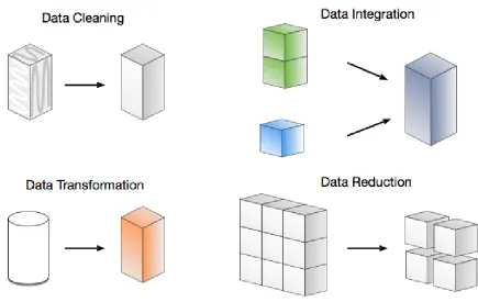
Figure 2.1: Data Preprocessing Categories
However, not all techniques may need to be used, depending on the data domain. Data
pre-processing can be grouped into four categories, as shown in Figure2.1: data cleaning, data transformation,data integration, anddata reduction.
Data Cleaning
Data cleaning focusses on handling missing, noisy, and inconsistent data. These characteristics
are typical of real-world datasets. Missing values can occur for several reasons. For instance,
an operator filling out a customer information form could skip some fields to make the process
quicker; some fields are simply not applicable to all customers; or an equipment malfunction
could lose a couple of records. Other malfunctioning equipment can record wrong values, or
an issue may happen during data transmission, including some outliers in the dataset.
Further-more, discrepancies in code or naming conventions can result in inconsistencies in the dataset.
Data cleaning techniques try to fill in missing values, smooth noisy data, identify and
re-move outliers, and resolve inconsistencies. Overall, machine learning algorithms can deal with
some level of “dirty” data, but the methods are not very robust, nor do they address all types of
issues. Some of the methods used to address each of these issues are described below.
1. Missing values: Not addressing this issue may lead to inaccurate models [13]. Various approaches can be used to handle missing values [14]. For example:
• Manually fill in missing values: this can be feasible if there are few missing values;
• Eliminate or ignore missing values[15]: this is straightforward to implement, but impractical unless most attributes of the entries are missing;
• Estimate missing values: a constant can be used, or the mean of all entries. An-other option is to use the expected value based on statistical methods [16] or An-other
prediction approaches.
2. Noise: this is a random error that modifies the original value. Noisy data can generate outliers as well. This issue has an impact on model accuracy and needs to be tackled [17].
In the case of noisy data, the following methods may be used:
• Inspection: a human operator can check the values after they are detected;
• Binning: sorting all the data values and splitting them into bins with the same number of entries. Next, the bins are smoothed using the bin values or the values
around them (e.g., using the mean);
• Clustering: clustering the data into normal and anomalous values and removing the anomalous ones;
• Regression: fitting the data with regression functions to smooth them.
2.1. Background 9
If there are known constraints, automated tools may find data that do not respect these
constraints.
Data Integration
Data integration is the process of merging data from multiple data sources. This process can
be tricky and must be performed carefully to avoid inconsistency and redundancy. The main
tasks of data integration are identifying and matching attributes, analyzing their correlation,
and detecting any conflict between the various data sources.
Data Transformation
Data transformation is the process of transforming or consolidating data into an appropriate
format for more efficient use. Data transformation techniques can be grouped into:
1. Aggregation: data aggregation can involve merging multiple attributes into a single at-tribute or combining two or more entries into a single entry. For example, individual
transactions can be aggregated to daily sales;
2. Normalization: Normalization means adjusting attribute values measured on different scales to a common scale. Normalization attempts to give equal weights to all attributes.
Some machine learning algorithms will not work properly without normalization.
Min-Max, expressed in Eq. (2.1), is a popular normalization method:
min−max= x−Xmin Xmax−Xmin
(2.1)
where x is the entry value, Xmin is the minimum value in the dataset, and Xmax is the
maximum value in the dataset;
Data Reduction
Data reduction includes various methods to obtain a reduced representation of the original
dataset while maintaining its properties and any existing intrinsic knowledge. Extracting the
same insights from the reduced dataset should also be possible. Usually, data reduction comes
with some degree of loss, and the trade-offmust be taken into consideration. The main
tech-niques used are:
1. Feature Selection: not all data features have the same importance, and feature selection techniques try to select the ones that best represent the data [18];
2. Instance Selection[19]: instead of selecting a subset of the features, instance selection tries to select a subset of instances to represent the full dataset;
3. Discretization[20]: this technique projects continuous attributes into a discrete domain, using non-overlapping ranges, for example.
2.1.2
Machine Learning
This section provides an overview of machine learning, focusing on the algorithms used in the
UCAP framework. Initially, a high-level overview of machine learning will be presented. Later
on, the concepts of theK-Meansand theGradient Boostingalgorithms are discussed. Overview
Machine learning is a part of artificial intelligence that explores algorithms that can receive
input data and use statistical analysis to predict an output value within acceptable accuracy.
Machine learning techniques usually share a similar process. It starts with a dataset, which
can be seen as a table where the rows represent observations and the columns are the values of
the observed attributes. The dataset is split into at least two subsets, the training dataset and
2.1. Background 11
process. Other dataset splitting schemes [21, 22] exist, but will not be discussed here because
they are out of the scope of this thesis.
In machine learning, the training process involves optimizing the parameters of a function,
called the loss or cost function. The function and the parameters vary depending on the
al-gorithm, but the goal is to minimize or maximize the loss function output when the model is
applied to the training dataset. Once the model is optimized, it is then evaluated using the test
dataset.
Machine learning algorithms are usually classified into three categories, according to the
learning process used: supervised learning, unsupervised learning, and reinforcement learning.
In supervised learning, the algorithm learns from a training set that contains the desired output values (labels) [23]. The objective is to build a model that can predict the correct output
for unseen data. This is analogous to the process in which a student learns from examples
provided by a teacher. The student must generalize the examples into rules or functions that
are applied when new examples arise.
Supervised learning is used primarily for two types of problems: classification problems and regression problems. In classification problems, the data have discrete labels. Each label
can be seen as a category or a class, and the goal is to build a model that can assign new data
entries to the most appropriate class. On the other hand, regression problems involve data
with continuous labels, rather than the discrete classes in classification problems. For example,
forecasting the energy consumption of a building is a regression problem.
In unsupervised learning [22], the training dataset does not contain any of the desired outputs. The algorithm’s objective is to find patterns in the data by itself. It tries to find some
intrinsic logic or rules that structure the training data. This is analogous to an individual who
tries to find similarities between objects or events to organize them into classes or categories
based on the individual’s perception rather than any pre-established categories. These types of
algorithms generate a better understanding of the data and provide insights into them. They
UCAP framework benefits from unsupervised learning.
Reinforcement learning is a type of learning in which the algorithm works as an agent that interacts with the environment, receiving feedback and adjusting its output accordingly.
It is used mainly in decision-making problems, where the decisions cause consequences. It is
analogous to learning by trial and error.
Next, two algorithms used in this work are detailed.
K-Means Algorithm
The K-means [24] is an unsupervised learning algorithm used to cluster unlabeled data. Its
goal is to assign the data intokclusters based on the available features.
The algorithm’s input is the data itself and the number of clustersk. The data samples ared -dimensional vectors (x1,x2, . . . ,xn) that will be assigned tok ≤ nclustersC1,C2, . . . ,Ck, with
nbeing the number of samples. The algorithm starts by choosingk centroids for the clusters (c1,c2, . . . ,ck), which are also d-dimensional vectors. The centroids could be, for example,
randomly selected data from the dataset. Then the algorithm iterates between the following
two steps:
1. Data samples are assigned to the cluster with the nearest centroid. Equation (2.2)
de-scribes this step. Thedist function computes the distance between two instances of the data, for example by using Euclidean distance.
Ci = {xj|dist(xj,cp)≥ dist(xj,ci),1≤ p≤k}. (2.2)
2. The centroids are updated by taking the average of all data samples assigned to each
cluster according to Eq. (2.3).
ci =
1
|Ci|
X
xj∈Ci
xj (2.3)
2.2. LiteratureReview 13
instance, when no data points change clusters or when some maximum number of iterations is
reached.
Gradient Boosting
Gradient boosting [25] is a boosting algorithm that uses gradient descent [26] to update its
predictors. Boosting is an ensemble approach in which the predictors are built sequentially.
The idea is that subsequent predictors learn from the mistakes of their predecessors. Ensemble
learning is a machine learning technique that uses multiple learners to solve a problem.
Gradient boosting algorithms use a loss function that varies according to the problem. For
instance, the mean squared error can be used as a loss function. Such algorithms also need
an ensemble of learners to make predictions, typically decision trees. Gradient boosting starts
with a single learner. Subsequent models predict the residual error of the previous models. The
prediction is given by the sum of all the models.
2.2
Literature Review
This section provides a literature review of research done on topics related to modelling user
behaviour based on location data.
The increasing amount of available location data has increased interest in building
predic-tion models around these data. One fundamental idea is that human mobility is predictable.
Songet al.[27] explored the limits of this predictability and found in their test population that 93% of human mobility was predictable. To reach this conclusion, they measured user entropy
from 45,000 mobile users.
Some studies have focussed on building models for next location prediction [3, 28, 29, 30,
31, 32].
the predicted category. They clustered users based on the frequency of visits using the K-Means
algorithm and built one prediction model per cluster. The category level captured the semantic
meaning of the user’s activities. After getting the predicted category from theHMM, they used a ranking scheme to predict the next-visited POI. They evaluated the impact of clustering on
the results and concluded that the clusters improved the results.
Noulaset al.[28] explored the problem of predicting the next-visited POI within 24 hours using check-in data. They proposed a set of features including user information, such as the
visits that a user has performed and visits performed by the user’s friends; global information
that aggregates data related to the POIs themselves, such as the distance between POIs and
existing transitions; and finally, they also used temporal features. These features were used to
evaluate a linear regression model and an M5 tree model with a dataset consisting of 35 million
check-ins from Foursquare. The M5 trees performed best in the evaluated metrics.
Preot¸iuc-Pietro and Cohn [29] studied the check-in patterns in LBSNs. Their features
con-sisted of the transitions that users make when they go from one POI to another. They clustered
the users based on their POI category transitions using theK−Meansalgorithm. They also built a model to predict the next POI category, inputting the same set of features to different Markov
models (MMs), and developed methods using the most frequent category over a period. Their results showed that higher-orderMMsdid not achieve improvement over lower-order models. However, they did not merge the clustering with the prediction.
Trasartiet al.[30] proposed a system, calledMyWay, to predict users’ exact future position based on mobility profiles, which are based on the users’ trajectories. These trajectories were
constructed using the users’ raw position. However, the raw position data do not need to be
shared to make the prediction, reducing privacy risks. Moreover, these authors also proposed a
collective strategy to consider more individuals’ data, but this would be applied only with data
shared by users. Besides, they proposed a hybrid approach that mixes both strategies. MyWay
was evaluated with a dataset gathered for insurance purposes and consisting of 9.8 million car
2.2. LiteratureReview 15
Nguyen et al.[31] applied a variety of machine learning methods to the next-visited POI problem, such as Markov models, Support Vector Machines (SVM), and decision trees. In their work, they built an Android app to collect GPS data from users. They collected each user’s
position every five minutes. According to their results, theSVMalgorithm performed best. Chen et al. [32] presented three approaches based on Markov models: a global model, based on all trajectories; a personal model based on a specific user; and a regional model in
which trajectories were clustered to build cluster models. Their data were collected from the
traffic system and represented cars passing specific locations. Their evaluation showed that
their approach outperforms two other methods,VMMandWhereNext.
In contrast with these studies [3, 28, 29, 30, 31, 32], the proposed research focusses on
users’ current activity preferences, not on future locations. Moreover, the UCAP framework
clusters users based on the places they have been and uses this information as a feature for
the prediction model, rather than building one individual prediction model per cluster. Other
studies have focussed either on LBSN data or other types of data, whereas this study proposes
a framework that works with both LBSN and GPS data and uses external context to improve
the prediction model.
Other studies have explored various ideas such as predicting where a user will be at a
specific time with datasets other than LBSN data [6, 33, 34].
Caoet al.[6] presented a framework to predict the probability of a user visiting a specific location at a given time. They first evaluate the possibility of a user visiting a location and then
checked whether the user would visit a specific location. They evaluated their approach using
data from three different LBSN datasets.
Liu et al.[33] proposed a method to predict where a user will go next at a specific time. Their method is based on recurrent neural networks, which usually uses a single transition
matrix. However, they used two matrices: a time-specific and distance-specific transition
ma-trices. They have evaluated their model with data from a LBSN dataset and also a dataset of
Lvet al.[34] presented two models: (1) a spatial-temporal model and (2) a next-visited POI prediction model based on Hidden Markov Models. Their dataset was periodically gathered
from LTE control-plan traffic generated by user equipment, such as mobile phones and other
electronic devices. They clustered nearby locations to reduce oscillation and identified the most
important POIs from users to use in their models. They grouped users into four previously
established clusters based on their daily patterns. Their models outperformed the baseline
methods in the evaluation.
Unlike [6, 33, 34], this study does not try to predict where the user is going at a specific
time and also considers data sources other than LBSNs. Furthermore, it is not restricted by
any sampling periodicity scenario. The UCAP framework can use data with either static or
variable sampling frequency. Also, the number of clusters is optimized when building a new
model, instead of using a previously established value. Moreover, other studies [6, 33, 34] do
not consider the external context, which may influence user behaviour.
Studies of building location recommender systems can be found in [35, 36, 37, 38]. Yao [35]
proposed a POI recommendation model based on Poisson factorization. The model first
pro-files the temporal popularity of the venues within one day and then matches the POI propro-files
with users’ preferences and routines. The users’ preferences and routines are gathered from a
LBSN dataset. The model can achieve improved evaluation over other factor-based models.
Yao et al. [36] used a tensor factorization check-in representation, with users, locations, and time slots as dimensions, to build a recommendation framework. They added social and
spatial regularization terms. The first of these was related to the users’ friends, whereas the
latter was related to the distance between the users’ check-ins. Yaoet al. evaluated their work using two datasets from two LBSNs and achieved better results than 12 other methods which
were used as the baseline.
He et al. [37] presented a model to handle location group recommendations. They took individual preferences into consideration and then used several factors to select recommended
Op-2.2. LiteratureReview 17
timality. They evaluated their idea using two datasets gathered from LBSNs, and their results
showed improvements over baseline models.
Capdevila et al. [38] presented a hybrid recommender system for geolocated data. They gathered data from Foursquare using a parallel version of the Quadtree algorithm, which was a
clever way to overcome the limitations of the API. They used a hybrid approach, with textual
sentiment analysis for the collaborative-filtering recommendation part and aggregated reviews
by users for the content-based recommendation part.
The UCAP framework could be extended to perform recommendations, but this was not
the main goal of this work, unlike the studies mentioned above [35, 36, 37, 38]. In addition,
these studies did not consider any context other than social relations, location, and time.
Lianet al.[39] presented a problem consisting of two tasks. First, they predicted whether users are willing to explore unvisited POIs. They evaluated a logistic regression and a
classi-fication and regression tree for this problem. Then, the result is used to choose the approach
taken to predict of the next-visited POI. If the users were willing to explore a POI they have
never visited, the researchers used a recommender system to find the best matches. If the user
was more likely to go to a POI where he/she had already been, a Markov Model and a temporal
regularity model were input into the Hidden Markov Model. Their system considered only
LBSN data, whereas the system proposed here is not restricted to such data.
Finally, Yang et al. [2] considered spatial and temporal dimensions for modelling user preferences (STAP). They built models for these dimensions separately and then merged them using a fusion framework. Furthermore, they used a tensor factorization model to exploit the
similarities among users. Their study was similar to this one, and their dataset and results
were used to evaluate the UCAP framework. In addition, UCAP considers not only spatial and
temporal information, but also the external context, such as temperature and wind conditions,
because it may affect user preferences. Moreover, their evaluation was performed based on
LBSNs datasets, whereas this study also considers datasets gathered without any user
mining, temporal, spatial, and spatial-temporal approaches.
2.3
Summary
This chapter provides an overview of the concepts related to various topics that assist in
un-derstanding the UCAP framework. More specifically, an introduction to data preprocessing
terminology has been presented. In addition, an introduction to machine learning and the
al-gorithms that are used in this research has been provided. Finally, current studies on various
topics related to modelling user behaviour based on location data were discussed and contrasted
to the methods used in the UCAP framework, which is the approach presented in this thesis.
Chapter 3
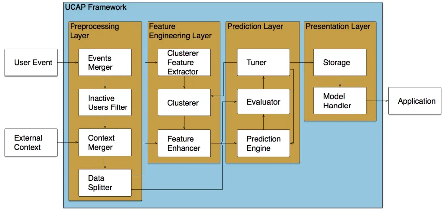
UCAP Framework
This chapter describes the proposed framework. The primary goal of the UCAP framework
is to build a model for predicting users’ current activity preferences based on their current
context. Figure 3.1 shows the data flow inside the UCAP framework.
The UCAP framework consists of four layers: thePreprocessing Layer, theFeature Engi-neering Layer, the Prediction Layer and the Presentation Layer. Feature engineering can be seen as part of the data preprocessing, but as UCAP adjusts the features along with the
predic-tion model, the feature engineering process is represented as a separate layer. The four layers
ensure better separation of responsibilities and help to decouple the functionalities from each
other.
The following sections explain each layer and its components and how each fits into the
framework.
3.1
Preprocessing Layer
The Preprocessing Layer is the framework’s input interface and the first step in training the prediction model. Two datasets serve as inputs to this layer: a User Event dataset and an
External Contextdataset.
Figure 3.1: Data flow of the UCAP Framework
• Unique user identifier (collected according to privacy policies)
• Location
• Timestamp
• Activity
The exact elements of the External contextdataset are not enforced by the UCAP frame-work as it cannot know a priori which and how many external contextual attributes will be used, but it should contain:
• Location
• Timestamp
• Context 1
• . . .
3.1. PreprocessingLayer 21
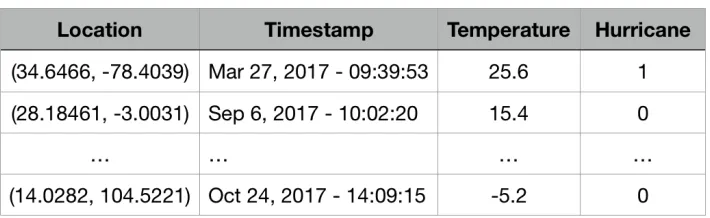
Figure 3.2: UCAP inputs example.
Figure 3.2 shows two example datasets: a User Event dataset and an External Context
dataset. TheExternal Contextdataset contains two contextual attributes: the temperature and whether a hurricane is present in an area or not, represented as 1 and 0, respectively.
The User Event dataset will most likely be gathered from online interaction with digital content, either as user input, such as the check-ins or without any user interaction, for example,
by a background process that stores the user location from time to time. The data gathered
with user interaction may contain duplicates, while the data gathered from background location
services may contain uncertainty, as it was shown in Fig. 1.1 and explained in Chapter 1. Both
scenarios are handled by thePreprocessing Layer.
Thecontextfrom anExternal Contextdataset may consist of numbers or labels. Each data type is processed differently by the Feature Engineering Layer. The Preprocessing Layer is concerned only with merging the context with the events according to the location and
times-tamp.
up of four components: theEvents Merger, theInactive Users Filter, theContext Merger, and theData Splitter. These components are detailed below.
3.1.1
Events Merger
The Events Merger component is a data aggregation component data allows that the UCAP framework to accept as aUser Eventdataset both LBSN check-in datasets and datasets gathered using background location services. This component is responsible for dealing with duplicates
generated by user input and multiple entries generated by GPS uncertainty.
Figure 3.3 (a) shows an example of aUser Eventdataset with both issues. The first two en-tries have the same user, location, timestamp, and activity. They represent duplicates generated
by user input. The last three entries have the same user, location, and timestamp, but different
activities. They depict entries generated by GPS uncertainty.
The Events Merger component merges all the events from a user with the same location and the same timestamp into a single event by changing its data representation. First, this
component takes the set of all activities performed by a user in a specific location and at a
specific timestamp. There are no duplicates in a set, which solves the user input duplication
problem.
Next, the Events Merger component changes the activity data representation. The User Eventdataset uses labels to represent activities performed by a user at a specific location and timestamp, such as the example given in Fig. 3.3 (a). Multiple entries may exist in the dataset
due to GPS uncertainty. Probabilities are a good representation of uncertainty, and theEvents Mergercomponent uses them to represent multiple activities performed by the same user with the same location and timestamp. All the activities performed in an event have the same
prob-ability, and their sum is one. Fig. 3.3 (b) depicts the output of this component, given Fig. 3.3
(a) as input. This new data representation solves the issue generated by GPS uncertainty.
Finally, a new issue arises with this representation. An event may become irrelevant if
3.1. PreprocessingLayer 23
activities than a particular thresholdn, the component uses a unique activityκto represent all the activities. Only this activity is performed in this case. The thresholdnis a parameter of the
Events Mergercomponent. Fig. 3.3 (c) gives the output of this component, given Fig. 3.3 (a) as input andn=2 as the threshold.
3.1.2
Inactive Users Filter
In this study, users were considered to have two kinds of status: active and inactive. Active
and inactive users were differentiated based on the frequency of each user’s events during a
period. Inactive users provide no value from the application perspective and affect negatively
the dataset as “dirty” data.
The UCAP framework is flexible regarding this frequency because the definition of an
active user may vary depending on the business domain. For example, an application that
shows the daily news can expect to be used daily by active users, but a sports results application
could define a user as active who used it once a week.
TheInactive Users Filter is a component that performs data cleaning by removing events related to inactive users from the User Event dataset. First, the time during which events happen is split into time intervals of the same duration, building a setT ={t0,t1, . . . ,tl}, where
the duration can be one day or one month, for example. Next, given E, the set containing all events; U, the set of all users; and Eu,t, the set of events that a useru ∈ U performed during
the time windowt ∈ T, the set of active usersU0 can be built according to Eq. (3.1). A user is considered to be active if the user generatesmor more events per defined time window. For example, to apply the equation to the news application example, the time window would be set
to one day, andm=1. TheInactive Users Filter will remove any event from a user who is not inU0.
3.1. PreprocessingLayer 25
Figure 3.4: Example of: (a) External Context dataset; (b) Context Merger being performed
3.1.3
Context Merger
The UCAP framework assumes that users’ activity preferences are not only related to
spatial-temporal attributes, but also to the external context. For example, severe weather conditions
may make outdoor activities challenging to perform. Moreover, special occasions such as the
Olympic Games influence the human behaviour in the place they occur and therefore should
be taken into account. For example, Fig. 3.4 (a) depicts an External Context dataset with information related to weather.
TheContext Mergercomponent integrates theExternal Contextdataset with theUser Event
dataset, which has already been preprocessed. It performs a data integration process, merging
them into a unique dataset. For instance, Fig. 3.4 (b) shows this component merging theUser Eventdataset from Fig. 3.3 (c) with theExternal Contextdepicted by Fig. 3.4 (a).
3.1.4
Data Splitter
validation dataset is used to evaluate this model and help select its parameters.
The Data Splitter orders the data chronologically to represent the most current user be-haviour and then uses the first q% as training dataset and the last (100− q)% as validation dataset, with 0≤ q≤100. The split is done this way because the prediction model will be used along with data that are more recent than the training dataset. Hence, this scenario is replicated
with the validation dataset.
3.2
Feature Engineering Layer
The results of prediction techniques are often improved by using newly generated features
based on existing ones. TheFeature Engineering Layer transforms the dataset received from thePreprocessing Layerby encoding it properly and merging it with newly generated features. It has two outputs:
• the training dataset with the new set of features themselves; and
• the data transformers that generated these features, i.e., the operations used to generate
the features. Other layers may apply these data transformers in other datasets.
The Feature Engineering Layeris composed of three components: the Clusterer Feature Extractor, theClusterer, and theFeature Enhancer. These components are described below.
3.2.1
Clusterer Feature Extractor
The first feature that the UCAP framework generates is related to the cluster to which each
user belongs. The clustering process is described in the next subsection. However, the critical
point, for now, is the fact that the clustering is based on the weighted frequency of activities
3.2. FeatureEngineeringLayer 27
being used by the clustering algorithm. TheClusterer Feature Extractoris the component that performs this task.
TheClusterer Feature Extractor faces two challenges. The first challenge is not knowing how many events a useruperformed. Counting may result in, for example, 5 events from user
u1and 5,000 from useru2. Because this unknown gap between results can influence the model
training, the numbers will be scaled to a known interval. The second challenge involves the
uncertainty of how often a user performs an activity. For instance, let activity a1 be “having
lunch”, and activity a2 be “going to school”. Almost every user would perform a1, whereas
only a fraction of users would performa2. Hence,a1 is not a useful feature for distinguishing
users, whereasa2could distinguish “students” from “non-students”.
To deal with the gap discrepancy between the total number of events and the fact that some
activities may be better metrics than others for distinguishing users, the UCAP uses a weighting
scheme. This weighting scheme is inspired by a widely used technique in information retrieval
and text mining,TF-IDF (Term Frequency-Inverse Document Frequency) [40]. In text classi-fication, documents have different lengths, and each text is written both with common words,
such as “the”, “and”, “or”, and words that are specific to a topic, for example, “algorithm”,
which would be related to “computer science”. This idea was adapted as follows: each useru
was considered as a document, and each activityaas a word. An event performed by a user at a specific timestampeu,tcontains a set of activities,Eurepresenting the set of events generated
by useruwith cardinality|Eu|. Equation (3.2) defines thet f function, which can be described
as the ratio of the number of times that user u performed an activitya over all the activities
u has performed. This equation deals with the first challenge described above. The second challenge is addressed by the functionid f(a), shown as Eq. (3.3). In this equation,U is the set of all users, andAu is the set of activities performed by useru. Thet f-id f function, shown in
Eq. (3.4), combines the two previous equations. This equation is used to build the dataset used
t f(a,u)= |{eu,t ∈Eu |a∈eu,t}|
|Eu|
(3.2)
id f(a)=log |U|
|{u∈U |a∈Au}|
(3.3)
t f-id f(a,u)=t f(a,u)×id f(a) (3.4) Suppose that user u1 from the example performed activity a1 twice and a2 three times,
whereas user u2 performed activity a2 in all 5,000 events. In this case, the t f function is
calculated as t f(a1,u1) = 52, t f(a2,u1) = 53, t f(a1,u2) = 0, and t f(a2,u2) = 1. Next, theid f
function is computed asid f(a1) = log21 = 0.301 andid f(a2) = log 1 = 0. Finally, thet f-id f
function results are t f-id f(a1,u1) = 0.0602 and t f-id f(a1,u2) = 0. Notice that id f(a2) = 0
means that this activity is not useful to differentiate users.
3.2.2
Clusterer
In addition to the issues regarding the number of events that a user may have performed, there
is the fact that these events may be sparse in time and also may present a data scarcity problem
because the number of activities performed per user is usually only a fraction of all the possible
activities [41]. Time is a fundamental feature of the UCAP framework, and there can be many
gaps in users’ daily routines in the datasets. To fill these gaps, users with similar preferences are
considered to have a similar routine. By clustering these users, their events can be considered
under a single entity, the “group of users”, rather than as individuals. For example, “parents”,
“university students”, and “hikers” could each cluster several individuals. Another advantage
of this approach is that new users can fit into a cluster after a few events and use a model that
is already built and trained.
3.2. FeatureEngineeringLayer 29
perform the existing activities weighted by theClusterer Feature Extractorcomponent. Users in the same cluster are supposed to exhibit similar behaviour regarding activities, and for this
reason, the cluster itself is a feature used by thePrediction Layer. This component builds and outputs a set of tuples with the users and the cluster to which each belongs.
3.2.3
Feature Enhancer
This component receives as input the data from both theClustererand thePreprocessing Layer. The data may contain features that are not encoded appropriately.
The data provided by the Clusterer are composed of tuples with a unique user identifier and an integer representing the cluster to which this user belongs. The user identifier is used to
merge these data into the feature set, but it is not a feature by itself. The number that identifies
the cluster is a feature to be included in the feature set.
Each cluster represents an entirely independent category of users. This kind of feature is
called a categorical feature. If an integer is used to represent each cluster, thePrediction Engine
can assume, for example, that cluster 1 and 2 are more similar than clusters 1 and 5. Moreover,
it assumes some ordering between clusters, which is not true. The approach taken is to create
one feature per cluster. This way, if there arekclusters, they will be represented bykfeatures. This representation is called1-of-Kscheme [42], and it is used to encodekmutually exclusive states, the clusters in this case. For example, if there are three clusters and a user belongs to
cluster 3, this user’s cluster is represented by (0,0,1).
The context from the External Context dataset may consist of numeric values or labels. Numerical values do not need any modifications. Labels are categorical features and use the
1-of-K representation. The Feature Enhancer does not care about what each context is but simply adjusts the data representation if needed.
Spatial features such as latitude and longitude are numeric values and do not need any
adjustment. These features represent the location where an event occurs and are fundamental
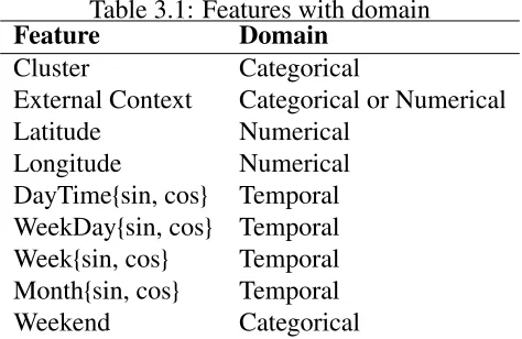
Table 3.1: Features with domain
Feature Domain
Cluster Categorical
External Context Categorical or Numerical
Latitude Numerical
Longitude Numerical
DayTime{sin, cos} Temporal WeekDay{sin, cos} Temporal Week{sin, cos} Temporal Month{sin, cos} Temporal
Weekend Categorical
Temporal features, based on the events’ timestamps, receive a different treatment. Several
features are generated based on them. The periodic temporal features are projected onto a unit
circle, using their sine and cosine as their representation, to maintain their properties. This
transformation is done using Eq. (3.5). In this equation, t represents the original temporal feature, andωtis its frequency.
ˆ
t=nsin 2πtωt,cos 2πtωt
o
(3.5)
This approach helps deal with frequency boundaries. For example, a day has 1,440
min-utes. By using Eq. (3.5), the distance between minute 1,439 and minute 0 is the same as the
difference between minute 0 and minute 1. If the original featuretwere used, there would be a considerable gap between these numbers.
Besides the periodic temporal features, there is a categorical feature indicating whether the
timestamp is on a weekday or a weekend. The set of features is summarized in Table 3.1.
3.3
Prediction Layer
The Prediction Layer deals with training a prediction model, evaluating it, and running the validation process to tune its parameters. This layer has two types of inputs: data and data
3.3. PredictionLayer 31
ThePrediction Layerreceives the feature set generated by theFeature Engineering Layer
(based on the training dataset) and the validation dataset from the Data Splitter component. The validation dataset is encoded using the data transformers received from theFeature Engi-neering Layer. These data transformers are the same as those used on the training dataset.
This layer is composed of three components: thePrediction Engine, theEvaluator, and the
Tuner. These components are described in the following subsections.
3.3.1
Prediction Engine
The Prediction Engine trains a model to predict which activities users will most likely per-form based on their current context. Its output is the trained prediction model. It receives the
feature dataset built by the Feature Enhancer component and uses it along with the activity probabilities computed by theEvents Mergercomponent.
This trained model outputs predicted activity probabilities ˆabased on the objective function shown in Eq. (3.6), wherelis the loss function,ais the ground truth, i.e., the probability vector computed by the Events Merger, and Ω is the regularization function, which represents the complexity of the model. The indexnis the size of the training dataset. The functionL is to be minimized.
L(model)=
n
X
i=1
l(ai,aˆi)+ Ω(model) (3.6)
3.3.2
Evaluator
The trained model must be evaluated to tune the training parameters. TheEvaluatoruses the data transformation processes generated by theFeature Engineering Layer, the model trained by thePrediction Engine, and the validation dataset received from theData Splitterto evaluate the model. Various evaluation metrics are computed in the experiments for study purposes, but
is computed as the ratio of correct predictions to the total number of predictions made.
3.3.3
Tuner
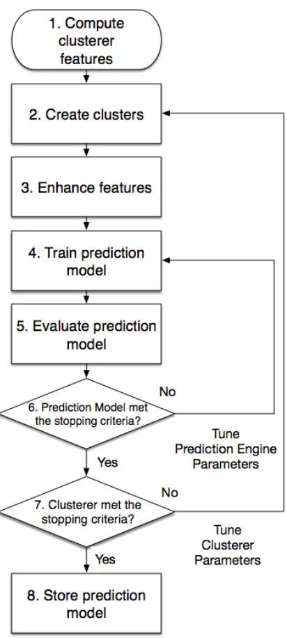
TheTunercoordinates the prediction model paramater tuning process. This process, depicted in Fig. 3.5, involves components from both theFeature Engineering Layerand thePrediction Layer.
The UCAP framework takes into consideration that clustering techniques may have
param-eters that can be tuned. This ends up including both theClusterercomponent and theFeature Enhancerin the tuning process. This process starts when theClusterer Feature Extractorsends the clusterer features (step 1). Next, clusters are created by theClusterer(step 2). The features are then encoded by theFeature Enhancer (step 3). The enhanced features are sent from the
Feature Engineering Layer to the Prediction Layer and used in the training process by the
Prediction Engine(step 4). The model is evaluated by theEvaluatorusing the validation data (step 5). The Tunercomponent keeps track of the evaluation results. If the stopping criteria were not met, it sends new parameters either to theClusterer(step 6) or thePrediction Engine
(step 7). A stopping criterion can be, for example, the number of iterations or the convergence
of a function whose input is the evaluation results. When the process is done, theTunersends the trained model to be stored (step 8). This process is also listed as pseudo-code in Algorithm
1. Notice that this component is generic and does not specify the tuning algorithm to be used,
which is specific to the implementation.
3.4
Presentation Layer
The Presentation Layer stores the trained model and all the data transformation processes needed by the prediction model; it can also run the prediction model on new data. This layer is
3.4. PresentationLayer 33
Algorithm 1:Simplified Tuning Process
input :trainData,validData
output:Clusterer Feature Extractor Data Transform
output:Trained Clusterer
output:Prediction Feature Extractor Data Transform
output:Trained Prediction Model
output:Training Results
1 o←Tuner();
2 clFE←ClusterFeatureExtractor(trainData); 3 clData←clFE.getData();
4 whileo.clusterStoppingCriteria()is falsedo
5 cl←Cluster(o.clParams(),clData);
6 PredFE←PredictionFeatureExtractor(trainData,clData,cl); 7 predData←PredFE.getData();
8 whileo.predStoppingCriteria()is falsedo
9 pred←PredictionEngine(o.predParams(),predData);
10 eval←Evaluator(validData,clFE,cl,PredFE,pred);
11 o.EvalResults(eval);
12 end
13 end
14 o.storeModel(clFE,cl,PredFE,pred)
3.4.1
Storage
TheStoragecomponent receives and stores the results, data transformations, and trained mod-els generated by the Feature Engineering Layerand the Prediction Layer. The data transfor-mations and the trained models will later be used by the application to provide predictions.
TheStoragecomponent must be implemented in such a way that when a data transforma-tion or a trained model is requested, only the most recent version is retrieved.
3.4.2
Model Handler
3.5. Summary 35
3.5
Summary
Case Studies
This chapter presents the UCAP implementation and the experiments used to evaluate UCAP.
It starts with a description of the experimental environment and implementation details. Next,
the five datasets used in all the experiments are presented, analyzed, and discussed. Then this
chapter presents three experiments that evaluate the UCAP framework. Each experiment has
its objectives detailed, as well as the metrics being used. Moreover, this chapter provides a
discussion of the experimental results. This chapter is organized into two sections. The first
will present the implementation and the experiments, and the second will present a discussion
of the experimental results.
4.1
Implementation and Experiments
The UCAP framework was implemented using Python. The experiments were run on a server
with 24 Intel Xeon CPUs at 2.60 GHz and 96 Gb RAM.
This section describes the shared components; experiment-specific component
implemen-tations are described in the subsection on that experiment.
4.1. Implementation andExperiments 37
Table 4.1: XGBoost Parameters
Parameter Value
Minimum Child Weight 50
ETA 0.1
Colsample by Tree 0.9
Maximum Depth 6
Subsample 0.9
Lambda 1.0
Booster gbtree
Objective binary:logitraw
Gamma 0
Clusterer
The Clusterer component uses theK-Means implementation from Scikit-learn [43] with Eu-clidean distance. TheK-Meansalgorithm was used due to its simplicity and effectiveness.
Other distances could have been used, but studies have shown that for high-dimensional
data spaces, results are similar [44]. Different clustering techniques were initially considered,
but preliminary tests showed that their performance was similar.
Prediction Engine
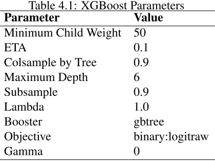
A gradient-boosting technique called eXtreme Gradient Boosting (XGBoost) [45] was used
as the prediction engine. To the best of the author’s knowledge, this is the first time that this
algorithm has been used in this problem domain.
Overall, tree-based methods are highly accurate and easy to use and to interpret. In
partic-ular, XGBoost was involved in 17 out of 29 challenge-winning solutions at Kaggle1 in 2015
[45]. This algorithm was used to minimize the objective function given in Eq. (3.6). Table 4.1
shows the parameters used by the XGBoost model.
The XGBoost algorithm does not output the required predicted activity probabilities, but
rather scores. These scores are related to how likely each activity is to be performed by the
they are input to the softmax function[42] usingσas described by Eq. (4.1). In this equation,
ais an activity, Athe set of all existing activities, andza is the score of activitya. The softmax
result for each entry in the dataset is the output of the prediction model. ThePrediction Engine
output is the output of Eq. (4.1).
σ(za)=
eza
P
a0∈Aeza0
(4.1)
Tuner
A grid-search approach was implemented as theTunercomponent, and it helped choosing the number of clusters for theK-Meansalgorithm.
4.1.1
Data Analysis
The experiments used five datasets, which are described in Table 4.2. TheLDN Smalldataset, theMTLdataset, and theLDN Largedataset were provided by a multi-media company special-ized in weather-related content and technology. All the data contained anonymspecial-ized
pseudo-identifiers and were collected in accordance with privacy policies. No personally identifiable
information about users was used. TheNYCand theTKY datasets were gathered as described in [2].
TheExternal Contextdataset consisted of temperature, wind speed, and weather condition, such as “Thunderstorm”, “Clear”, or “Snow Showers”. For London, ON, these data were
extracted from the Canadian Historical Climate Data2. For New York and Tokyo, these data
were obtained through the Weather Undergroung API3.
Figures 4.1, 4.2 and 4.3 were plotted to depict the datasets more clearly. Figure 4.1 shows
the probability distribution of the number of events per user in the datasets. The shape of the
curves is very similar for all datasets, where most users have very few events. A successful
4.1. Implementation andExperiments 39
Table 4.2: Datasets Description
Dataset LDN Small LDN Large MTL NYC TKY
Location London, ON London, ON Montreal New York Tokyo
Canada Canada
Data Source GPS GPS GPS LBSN LBSN
Start Date March 19th June 12th March 19th April 12th April 12th
2017 2017 2017 2012 2012
End Date May 2nd October 19th May 2nd February 16th February 16th
2017 2017 2017 2013 2013
Number of 2,481,358 76,098,559 11,782,099 227,428 573,703
Events
Unique 40,781 129,609 196,100 824 1,939
Users
Unique 77 84 72 251 251
Activities
approach to any problem that uses location data needs to handle this scenario. Figure 4.2
displays the number of events as a time series. Highlighting the different timeframes between
the datasets is good, whereas theNYCandTKY datasets covered about ten months of data, the other two contained only about two months of data and may seem smoother, although they are
not. Finally, Fig. 4.3 gives the plot of the number of activities per event. Each event is related
to a unique user in a specific timestamp. The difference between the LBSN dataset, which
presents a single activity per event for all the events, and the GPS datasets are noticeable.
4.1.2
Experiment 1: Impact of the UCAP Components
The objective of this experiment was to evaluate the impact of the main components used by
the UCAP framework. The evaluation process used five variations of the framework: UCAP
without the Events Merger, UCAP without the Inactive Users Filter, UCAP without Exter-nal Context, UCAP without the Clusterer, and finally UCAP with all its components. Each variation of the framework used in this experiment was trained independently.
The set-up used the LDN Small dataset. The value used for the parameter m from the
4.1. Implementation andExperiments 41
4.1. Implementation andExperiments 43
Table 4.3: Experiment 1 Results
Model Accuracy RMSE MAE
No Inactive Users filter 0.95 0.09 0.087
No Events Merger 0.89 0.17 0.032
No External Context 0.96 0.08 0.0083
No Clusterer 0.91 0.09 0.0082
UCAP 0.97 0.08 0.0079
meant that any user who performed five or more events was considered active.
The data were ordered chronologically, the first 80% of the data were used as the training
dataset, and the last 20% were used as the test dataset. TheData Splitterseparates the training dataset into a training dataset and a validation dataset during the training process. The test
dataset is used only for the evaluation.
To compare the performance of the models, the following metrics were used: (a)Accuracy, used by theEvaluator component; (b) the Root Mean Square Error (RMSE), according to Eq. (4.2); and (c) the Mean Absolute Error (MAE), according to Eq. (4.3).
ForAccuracy, the higher the number, the better, and 1 is the highest score. ForRMSE(Eq. (4.2)), the lower the score, the better, and 0 is the best possible value. In this equation,Ais the dataset with all the ground truths, and ˆAis the dataset with the predictions,a ∈ A, ˆa ∈ Aˆ, and
n = |A| = |Aˆ|. TheMAE(Eq. (4.3)) follows the same logic asRMSE: the lower the score, the better. Both equations used the same parameters.
RMS E(A,Aˆ)=
v t 1 n n−1 X
i=0
(ai−aˆi)2 (4.2)
MAE(A,Aˆ)= 1
n
n−1 X
i=0
abs(ai−aˆi) (4.3)
Figure 4.4 shows the results of this experiment, which are summarized in Table 4.3.
The UCAP framework with all the components and features presented a better performance
Figure 4.4: UCAP variations prediction results
improvement inAccuracy. Other components also provided relatively smaller improvements to the result, which gives evidence of their importance to the proposed approach.
4.1.3
Experiment 2: Comparison with a Di
ff
erent Approach
The objective of this experiment was to compare the proposed framework with a current
tech-nique that models the same problem to evaluate its effectiveness. Two datasets from [2] were
used, which were theLBSNdatasets described in Table 4.2. The UCAP framework was com-pared with their model, calledSTAP, by replicating their experimental set.
The value used for the parameter m from the Inactive Users Filter was 3, and the time window was one week, meaning that users were considered active if they generated at least
three events per week. The parameters used in the XGBoost model were the same as those in
Experiment 1, as shown in Table 4.1.
train-4.1. Implementation andExperiments 45
Figure 4.5: UCAP andSTAPcomparison Table 4.4: Experiment 2 Results
Model NYC TKY
STAP[2] 0.52 0.54
UCAP 0.59 0.60
ing dataset, the ninth month was used as the validation dataset, and the tenth month was used
as the test dataset. The test dataset is used only for the evaluation.
To compare the performance of the models, theAccuracymeasure was used. Table 4.4 and Fig.4.5 summarize the results of this experiment. The framework proposed here outperformed
the STAP model by 13.5% on accuracy on the NYC dataset and 11.1% on the TKY, or 12.3%
better by averaging these two values.
4.1.4
Experiment 3: Comparison between Di
ff
erent Datasets
The objective of this experiment was to compare the performance of the proposed framework
when applied to different datasets. This experiment used all five datasets described in Table 4.2.
It is good to highlight theLDN Largedataset, which could be consideredBig Dataconcerning its volume because the number of entries is large enough that the dataset does not fit entirely
in memory [46]. To address the size issue, Dask [47] was used in thePreprocessing Layer. For the datasets used in the previous experiments (LDN Small, NYC, andTKY), the entire set-up was kept the same. For the other two datasets, the MTL dataset and the LDN Large