Copyright2000 by the Genetics Society of America
Inference of Population Structure Using Multilocus Genotype Data
Jonathan K. Pritchard, Matthew Stephens and Peter Donnelly
Department of Statistics, University of Oxford, Oxford OX1 3TG, United Kingdom
Manuscript received September 23, 1999 Accepted for publication February 18, 2000
ABSTRACT
We describe a model-based clustering method for using multilocus genotype data to infer population structure and assign individuals to populations. We assume a model in which there are K populations (where K may be unknown), each of which is characterized by a set of allele frequencies at each locus. Individuals in the sample are assigned (probabilistically) to populations, or jointly to two or more popula-tions if their genotypes indicate that they are admixed. Our model does not assume a particular mutation process, and it can be applied to most of the commonly used genetic markers, provided that they are not closely linked. Applications of our method include demonstrating the presence of population structure, assigning individuals to populations, studying hybrid zones, and identifying migrants and admixed individu-als. We show that the method can produce highly accurate assignments using modest numbers of loci—e.g., seven microsatellite loci in an example using genotype data from an endangered bird species. The software used for this article is available from http://www.stats.ox.ac.uk/ⵑpritch/home.html.
I
N applications of population genetics, it is often use- populations based on these subjective criteria represents a natural assignment in genetic terms, and it would be ful to classify individuals in a sample intopopula-tions. In one scenario, the investigator begins with a useful to be able to confirm that subjective classifications are consistent with genetic information and hence ap-sample of individuals and wants to say something about
the properties of populations. For example, in studies propriate for studying the questions of interest. Further, there are situations where one is interested in “cryptic” of human evolution, the population is often considered
to be the unit of interest, and a great deal of work has population structure—i.e., population structure that is difficult to detect using visible characters, but may be focused on learning about the evolutionary
relation-ships of modern populations (e.g.,Cavalliet al. 1994). significant in genetic terms. For example, when associa-tion mapping is used to find disease genes, the presence In a second scenario, the investigator begins with a set
of predefined populations and wishes to classify individ- of undetected population structure can lead to spurious associations and thus invalidate standard tests (Ewens uals of unknown origin. This type of problem arises
in many contexts (reviewed by Davieset al. 1999). A andSpielman1995). The problem of cryptic population structure also arises in the context of DNA fingerprint-standard approach involves sampling DNA from
mem-bers of a number of potential source populations and ing for forensics, where it is important to assess the degree of population structure to estimate the probabil-using these samples to estimate allele frequencies in
ity of false matches (BaldingandNichols1994, 1995; each population at a series of unlinked loci. Using the
Foremanet al. 1997;Roederet al. 1998). estimated allele frequencies, it is then possible to
com-Pritchard and Rosenberg (1999) considered how pute the likelihood that a given genotype originated in
genetic information might be used to detect the pres-each population. Individuals of unknown origin can be
ence of cryptic population structure in the association assigned to populations according to these likelihoods
mapping context. More generally, one would like to be Paetkauet al. 1995;Rannala andMountain 1997).
able to identify the actual subpopulations and assign In both situations described above, a crucial first step
individuals (probabilistically) to these populations. In is to define a set of populations. The definition of
popu-this article we use a Bayesian clustering approach to lations is typically subjective, based, for example, on
tackle this problem. We assume a model in which there linguistic, cultural, or physical characters, as well as the
are K populations (where K may be unknown), each of geographic location of sampled individuals. This
subjec-which is characterized by a set of allele frequencies at tive approach is usually a sensible way of incorporating
each locus. Our method attempts to assign individuals diverse types of information. However, it may be difficult
to populations on the basis of their genotypes, while to know whether a given assignment of individuals to
simultaneously estimating population allele frequen-cies. The method can be applied to various types of markers [e.g., microsatellites, restriction fragment Corresponding author: Jonathan Pritchard, Department of Statistics,
length polymorphisms (RFLPs), or single nucleotide
University of Oxford, 1 S. Parks Rd., Oxford OX1 3TG, United
King-dom. E-mail: [email protected] polymorphisms (SNPs)], but it assumes that the marker
loci are unlinked and at linkage equilibrium with one observations from each cluster are random draws from some parametric model. Inference for the pa-another within populations. It also assumes
Hardy-Wein-berg equilibrium within populations. (We discuss these rameters corresponding to each cluster is then done jointly with inference for the cluster membership of assumptions further in background on clustering
methodsand thediscussion.) each individual, using standard statistical methods
(for example, maximum-likelihood or Bayesian Our approach is reminiscent of that taken bySmouse
et al. (1990), who used the EM algorithm to learn about methods). the contribution of different breeding populations to a
Distance-based methods are usually easy to apply and sample of salmon collected in the open ocean. It is also
are often visually appealing. In the genetics literature, it closely related to the methods ofForemanet al. (1997)
has been common to adapt distance-based phylogenetic and Roeder et al. (1998), who were concerned with
algorithms, such as neighbor-joining, to clustering estimating the degree of cryptic population structure
multilocus genotype data (e.g., Bowcock et al. 1994). to assess the probability of obtaining a false match at
However, these methods suffer from many disadvan-DNA fingerprint loci. Consequently they focused on
tages: the clusters identified may be heavily dependent estimating the amount of genetic differentiation among
on both the distance measure and graphical representa-the unobserved populations. In contrast, our primary
tion chosen; it is difficult to assess how confident we interest lies in the assignment of individuals to
popula-should be that the clusters obtained in this way are tions. Our approach also differs in that it allows for the
meaningful; and it is difficult to incorporate additional presence of admixed individuals in the sample, whose
information such as the geographic sampling locations genetic makeup is drawn from more than one of the K
of individuals. Distance-based methods are thus more populations.
suited to exploratory data analysis than to fine statistical In the next section we provide a brief description
inference, and we have chosen to take a model-based of clustering methods in general and describe some
approach here. advantages of the model-based approach we take. The
The first challenge when applying model-based meth-details of the models and algorithms used are given in
ods is to specify a suitable model for observations from models and methods.We illustrate our method with
each cluster. To make our discussion more concrete we several examples in applications to data: both on
introduce very briefly some of our model and notation simulated data and on sets of genotype data from an
here; a fuller treatment is given later. Assume that each endangered bird species and from humans.
incorpo-cluster (population) is modeled by a characteristic set rating population information describes how our
of allele frequencies. Let X denote the genotypes of the method can be extended to incorporate geographic
sampled individuals, Z denote the (unknown) popula-information into the inference process. This may be
tions of origin of the individuals, and P denote the useful for testing whether particular individuals are
mi-(unknown) allele frequencies in all populations. (Note grants or to assist in classifying individuals of unknown
that X, Z, and P actually represent multidimensional origin (as inRannalaandMountain1997, for
exam-vectors.) Our main modeling assumptions are Hardy-ple). Background on the computational methods used
Weinberg equilibrium within populations and complete in this article is provided in theappendix.
linkage equilibrium between loci within populations. Under these assumptions each allele at each locus in each genotype is an independent draw from the appro-BACKGROUND ON CLUSTERING METHODS
priate frequency distribution, and this completely speci-Consider a situation where we have genetic data from
fies the probability distribution Pr(X|Z, P) (given later a sample of individuals, each of whom is assumed to
in Equation 2). Loosely speaking, the idea here is that have originated from a single unknown population (no
the model accounts for the presence of Hardy-Weinberg admixture). Suppose we wish to cluster together
individ-or linkage disequilibrium by introducing population uals who are genetically similar, identify distinct clusters,
structure and attempts to find population groupings and perhaps see how these clusters relate to
geographi-that (as far as possible) are not in disequilibrium. While cal or phenotypic data on the individuals. There are
inference may depend heavily on these modeling as-broadly two types of clustering methods we might use:
sumptions, we feel that it is easier to assess the validity of explicit modeling assumptions than to compare the 1. Distance-based methods. These proceed by calculating
relative merits of more abstract quantities such as dis-a pdis-airwise distdis-ance mdis-atrix, whose entries give the
tance measures and graphical representations. In situa-distance (suitably defined) between every pair of
in-tions where these assumpin-tions are deemed unreason-dividuals. This matrix may then be represented using
able then alternative models should be built. some convenient graphical representation (such as a
Having specified our model, we must decide how to tree or a multidimensional scaling plot) and clusters
perform inference for the quantities of interest (Z and may be identified by eye.
by specifying models (priors) Pr(Z) and Pr(P), for both Assume that before observing the genotypes we have Z and P. The Bayesian approach provides a coherent no information about the population of origin of each framework for incorporating the inherent uncertainty individual and that the probability that individual i origi-of parameter estimates into the inference procedure nated in population k is the same for all k,
and for evaluating the strength of evidence for the
in-Pr(z(i)⫽k)⫽ 1/K , (3)
ferred clustering. It also eases the incorporation of
vari-ous sorts of prior information that may be available, independently for all individuals. (In cases where some such as information about the geographic sampling lo- populations may be more heavily represented in the cation of individuals. sample than others, this assumption is inappropriate; it Having observed the genotypes, X, our knowledge would be straightforward to extend our model to deal about Z and P is then given by the posterior distribution with such situations.)
We follow the suggestion of Baldingand Nichols Pr(Z, P|X)⬀Pr(Z)Pr(P)Pr(X|Z, P). (1)
(1995) (see also Foreman et al. 1997 and Rannala While it is not usually possible to compute this distribu- and Mountain 1997) in using the Dirichlet distri-tion exactly, it is possible to obtain an approximate bution to model the allele frequencies at each locus sample (Z(1), P(1)), (Z(2), P(2)), . . . ,(Z(M), P(M)) from Pr(Z,
within each population. The Dirichlet distribution P|X) using Markov chain Monte Carlo (MCMC) meth- D(
1,2, . . . ,J) is a distribution on allele frequencies
ods described below (seeGilks et al. 1996b, for more p⫽(p
1, p2, . . . , pJ) with the property that these
frequen-general background). Inference for Z and P may then cies sum to 1. We use this distribution to specify the be based on summary statistics obtained from this sam- probability of a particular set of allele frequencies p
kl·
ple (see Inference for Z, P, and Q below). A brief
introduc-for population k at locus l, tion to MCMC methods and Gibbs sampling may be
found in theappendix. pkl·ⵑD(1,2, . . . ,Jl), (4)
independently for each k,l. The expected frequency of MODELS AND METHODS allele j is proportional to j, and the variance of this frequency decreases as the sum of thejincreases. We
We now provide a more detailed description of our
take1⫽ 2⫽ · · ·⫽ Jl⫽1.0, which gives a uniform
modeling assumptions and the algorithms used to
per-distribution on the allele frequencies; alternatives are form inference, beginning with the simpler case where
discussed in thediscussion. each individual is assumed to have originated in a single
MCMC algorithm (without admixture):Equations 2, population (no admixture).
3, and 4 define the quantities Pr(X|Z, P), Pr(Z), and The model without admixture:Suppose we genotype
Pr(P), respectively. By setting ⫽(1,2)⫽(Z, P) and N diploid individuals at L loci. In the case without
admix-letting(Z, P)⫽ Pr(Z, P|X) we can use the approach ture, each individual is assumed to originate in one of
outlined in Algorithm A1 to construct a Markov chain K populations, each with its own characteristic set of
with stationary distribution Pr(Z, P|X) as follows: allele frequencies. Let the vector X denote the observed
Algorithm1: Starting with initial values Z(0)for Z (by genotypes, Z the (unknown) populations of origin of
drawing Z(0) at random using (3) for example), iterate the the individuals, and P the (unknown) allele frequencies
following steps for m⫽ 1, 2, . . . . in the populations. These vectors consist of the
follow-ing elements,
Step 1. Sample P(m)from Pr(P|X, Z(m⫺1)). (x(i,1)
l , x(i,2)l )⫽genotype of the ith individual at the l th locus, Step 2. Sample Z(m)from Pr(Z|X, P(m)).
where i⫽1, 2, . . . , N and l⫽1, 2, . . . , L;
z(i)⫽population from which individual i originated;
Informally, step 1 corresponds to estimating the allele pklj⫽frequency of allele j at locus l in population k,
frequencies for each population assuming that the pop-where k⫽1, 2, . . . , K and j⫽1, 2, . . . , Jl,
ulation of origin of each individual is known; step 2 where Jl is the number of distinct alleles observed at corresponds to estimating the population of origin of
locus l, and these alleles are labeled 1, 2, . . . , Jl. each individual, assuming that the population allele
fre-Given the population of origin of each individual, quencies are known. For sufficiently large m and c, (Z(m), the genotypes are assumed to be generated by drawing P(m)), (Z(m⫹c), P(m⫹c)), (Z(m⫹2c), P(m⫹2c)), . . . will be
approxi-alleles independently from the appropriate population mately independent random samples from Pr(Z, P|X).
frequency distributions, The distributions required to perform each step are
given in theappendix. Pr(x(i,a)
l ⫽ j|Z, P)⫽ pz(i)lj (2)
The model with admixture: We now expand our model to allow for admixed individuals by introducing independently for each x(i,a)
l . (Note that pz(i)ljis the
fre-a vector Q to denote the fre-admixture proportions for efre-ach quency of allele j at locus l in the population of origin
q(i)
k ⫽ proportion of individual i’s genome that tion of origin of each allele copy in each individual is
known; step 2 corresponds to estimating the population originated from population k.
of origin of each allele copy, assuming that the popula-It is also necessary to modify the vector Z to replace the
tion allele frequencies and the admixture proportions assumption that each individual i originated in some
are known. As before, for sufficiently large m and c, unknown population z(i)with the assumption that each
(Z(m), P(m), Q(m)), (Z(m⫹c), P(m⫹c), Q(m⫹c)), (Z(m⫹2c), P(m⫹2c),
observed allele copy x(i,a)
l originated in some unknown
Q(m⫹2c)), . . . will be approximately independent random population z(i,a)
l :
samples from Pr(Z, P, Q|X). The distributions required to perform each step are given in theappendix.
z(i,a)
l ⫽population of origin of allele copy x(i,a)l .
Inference: Inference for Z, P, and Q: We now discuss how We use the term “allele copy” to refer to an allele carried
the MCMC output can be used to perform inference on at a particular locus by a particular individual.
Z, P, and Q. For simplicity, we focus our attention on Q ; Our primary interest now lies in estimating Q. We inference for Z or P is similar.
proceed in a manner similar to the case without admix- Having obtained a sample Q(1), . . . , Q(M)(using suitably ture, beginning by specifying a probability model for large burn-in m and thinning interval c) from the poste-(X, Z, P, Q). Analogues of (2) and (3) are rior distribution of Q ⫽ (q
1, . . . , qN) given X using
the MCMC method, it is desirable to summarize the Pr(x(i,a)
l ⫽j|Z, P, Q)⫽ pz(i,a)
l lj (5)
information contained, perhaps by a point estimate of and Q. A seemingly obvious estimate is the posterior mean
Pr(z(i,a)
l ⫽k|P, Q)⫽q(i)k, (6)
E(qi|X)≈
1 M
兺
M
m⫽1
q(m)
i . (8)
with (4) being used to model P as before. To complete our model we need to specify a distribution for Q, which
However, the symmetry of our model implies that the in general will depend on the type and amount of
admix-posterior mean of qi is (1/K,1/K, . . . , 1/K) for all i,
ture we expect to see. Here we model the admixture
whatever the value of X. For example, suppose that there proportions q(i) ⫽ (q(i)
1, . . . , q(i)K) of individual i using
are just two populations and 10 individuals and that the the Dirichlet distribution
genotypes of these individuals contain strong informa-tion that the first 5 are in one populainforma-tion and the second q(i)ⵑD(␣,␣, . . . ,␣) (7)
5 are in the other population. Then either independently for each individual. For large values of
␣ (Ⰷ1), this models each individual as having allele q1. . . q5≈(1, 0) and q6. . . q10≈ (0, 1) (9) copies originating from all K populations in equal
pro-or portions. For very small values of␣(Ⰶ1), it models each
individual as originating mostly from a single popu- q1. . . q
5≈(0, 1) and q6. . . q10≈ (1, 0), (10) lation, with each population being equally likely. As
with these two “symmetric modes” being equally likely,
␣ → 0 this model becomes the same as our model
leading to the expectation of any given qi being (0.5,
without admixture (although the implementation of the
0.5). This is essentially a problem of nonidentifiability MCMC algorithm is somewhat different). We allow ␣
caused by the symmetry of the model [see Stephens to range from 0.0 to 10.0 and attempt to learn about␣
(2000b) for more discussion]. from the data (specifically we put a uniform prior on
In general, if there are K populations then there will
␣苸[0, 10] and use a Metropolis-Hastings update step
be K ! sets of symmetric modes. Typically, MCMC to integrate out our uncertainty in␣). This model may
schemes find it rather difficult to move between such be considered suitable for situations where little is
modes, and the algorithms we describe will usually ex-known about admixture; alternatives are discussed in
plore only one of the symmetric modes, even when run thediscussion.
for a very large number of iterations. Fortunately this MCMC algorithm (with admixture): The following
does not bother us greatly, since from the point of algorithm may be used to sample from Pr(Z, P, Q|X).
view of clustering all the symmetric modes are the same Algorithm2: Starting with initial values Z(0) for Z (by
drawing Z(0) at random using (3) for example), iterate the [compare the clusterings corresponding to (9) and following steps for m⫽1, 2, . . . . (10)]. If our sampler explores only one symmetric mode then the sample means (8) will be very poor estimates Step 1. Sample P(m), Q(m)from Pr(P, Q|X, Z(m⫺1)).
of the posterior means for the qi, but will be much better
Step 2. Sample Z(m)from Pr(Z|X, P(m), Q(m)).
estimates of the modes of the qi, which in this case turn
Step 3. Update␣using a Metropolis-Hastings step.
out to be a much better summary of the information in the data. Ironically then, the poor mixing of the Informally, step 1 corresponds to estimating the allele
MCMC sampler between the symmetric modes gives frequencies for each population and the admixture
value. Where the MCMC sampler succeeds in moving Simulated data:To test the performance of the clus-tering method in cases where the “answers” are known, between symmetric modes, or where it is desired to
combine results from samples obtained using different we simulated data from three population models, using standard coalescent techniques (Hudson1990). We as-starting points (which may involve combining results
corresponding to different modes), more sophisticated sumed that sampled individuals were genotyped at a series of unlinked microsatellite loci. Data were simu-methods [such as those described by Stephens
(2000b)] may be required. lated under the following models.
Inference for the number of populations: The problem of
Model 1: A single random-mating population of con-inferring the number of clusters, K, present in a data
stant size. set is notoriously difficult. In the Bayesian paradigm the
Model 2: Two random-mating populations of constant way to proceed is theoretically straightforward: place a
effective population size 2N. These were assumed to prior distribution on K and base inference for K on the
have split from a single ancestral population, also of posterior distribution
size 2N at a time N generations in the past, with no subsequent migration.
Pr(K|X)⬀Pr(X|K)Pr(K). (11)
Model 3: Admixture of populations. Two discrete popu-However, this posterior distribution can be peculiarly
lations of equal size, related as in model 2, were fused dependent on the modeling assumptions made, even
to produce a single random-mating population. Sam-where the posterior distributions of other quantities (Q,
ples were collected after two generations of random Z, and P, say) are relatively robust to these assumptions.
mating in the merged population. Thus, individuals Moreover, there are typically severe computational
chal-have i grandparents from population 1, and 4 ⫺ i lenges in estimating Pr(X|K). We therefore describe an
grandparents from population 2 with probability alternative approach, which is motivated by
approximat-(4
i)/16, where i苸{0, 4}. All loci were simulated
inde-ing (11) in an ad hoc and computationally convenient
pendently. way.
We present results from analyzing data sets simulated Arguments given in theappendix(Inference on K, the
under each model. Data set 1 was simulated under number of populations) suggest estimating Pr(X|K) using
model 1, with 5 microsatellite loci. Data sets 2A and 2B Pr(X|K)≈exp(⫺ˆ /2⫺ ˆ2/8), (12)
were simulated under model 2, with 5 and 15 microsatel-lite loci, respectively. Data set 3 was simulated under where
model 3, with 60 loci (preliminary analyses with fewer loci showed this to be a much harder problem than
ˆ ⫽ 1 M
兺
M
m⫽1
⫺2 log Pr(X|Z(m), P(m), Q(m)) (13)
models 1 and 2). Microsatellite mutation was modeled by a simple stepwise mutation process, with the mutation and
parameter 4Nset at 16.0 per locus (i.e., the expected variance in repeat scores within populations was 8.0).
ˆ2 ⫽ 1 M
兺
M
m⫽1
(⫺2 log Pr(X|Z(m), P(m), Q(m))⫺ ˆ )2.
We did not make use of the assumed mutation model in analyzing the simulated data.
(14)
Our analysis consists of two phases. First, we consider We use (12) to estimate Pr(X|K) for each K and substi- the issue of model choice—i.e., how many populations tute these estimates into (11) to approximate the poste- are most appropriate for interpreting the data. Then, rior distribution Pr(K|X). we examine the clustering of individuals for the inferred
In fact, the assumptions underlying (12) are dubious number of populations.
at best, and we do not claim (or believe) that our proce- Choice ofKfor simulated data:For each model, we dure provides a quantitatively accurate estimate of the ran a series of independent runs of the Gibbs sampler posterior distribution of K. We see it merely as an ad for each value of K (the number of populations) be-hoc guide to which models are most consistent with the tween 1 and 5. The results presented are based on runs data, with the main justification being that it seems of 106iterations or more, following a burn-in period of to give sensible answers in practice (see next section for at least 30,000 iterations. To choose the length of the examples). Notwithstanding this, for convenience we burn-in period, we printed out log(Pr(X|P(m), Q(m))), and continue to refer to “estimating” Pr(K|X) and Pr(X|K). several other summary statistics during the course of a series of trial runs, to estimate how long it took to reach (approximate) stationarity. To check for possible prob-APPLICATIONS TO DATA
lems with mixing, we compared the estimates of P(X|K) and other summary statistics obtained over several inde-We now illustrate the performance of our method on
both simulated data and real data (from an endangered pendent runs of the Gibbs sampler, starting from differ-ent initial points. In general, substantial differences be-bird species and from humans). The analyses make use
TABLE 1
Estimated posterior probabilities ofK, for simulated data sets 1, 2A, 2B, and 3 (denotedX1,X2A,X2B,
andX3, respectively)
K log P(K|X1) P(K|X2A) P(K|X2B) P(K|X3)
1 ⵑ1.0 ⵑ0.0 ⵑ0.0 ⵑ0.0
2 ⵑ0.0 0.21 0.999 ⵑ1.0
3 ⵑ0.0 0.58 0.0009 ⵑ0.0
4 ⵑ0.0 0.21 ⵑ0.0 ⵑ0.0
5 ⵑ0.0 ⵑ0.0 ⵑ0.0 ⵑ0.0
The numbers should be regarded as a rough guide to which models are consistent with the data, rather than accurate esti-mates of posterior probabilities.
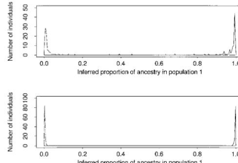
Figure1.—Summary of the clustering results for simulated data sets 2A and 2B, respectively. For each individual, we be longer to obtain more accurate estimates or that
computed the mean value of q(i)
1 (the proportion of ancestry independent runs are getting stuck in different modes in population 1), over a single run of the Gibbs sampler. The in the parameter space. (Here, we consider the K ! dashed line is a histogram of mean values of q(i)
1 for individuals from population 0; the solid line is for individuals from popula-modes that arise from the nonidentifiability of the K
tion 1. populations to be equivalent, since they arise from
per-muting the K population labels.)
We found that in most cases we obtained consistent
and Q estimating the number of grandparents from estimates of P(X|K) across independent runs. However,
each of the two original populations, for each individual. when analyzing data set 2A with K⫽3, the Gibbs sampler
Intuitively it seems that another plausible clustering found two different modes. This data set actually
con-would be with K ⫽ 5, individuals being assigned to tains two populations, and when K is set to 3, one of
clusters according to how many grandparents they have the populations expands to fill two of the three clusters.
from each population. In biological terms, the solution It is somewhat arbitrary which of the two populations
with K⫽ 2 is more natural and is indeed the inferred expands to fill the extra cluster: this leads to two modes
value of K for this data set using our ad hoc guide [the of slightly different heights. The Gibbs sampler did not
estimated value of Pr(X|K) was higher for K ⫽5 than manage to move between the two modes in any of our
for K ⫽ 3, 4, or 6, but much lower than for K ⫽ 2]. runs.
However, this raises an important point: the inferred In Table 1 we report estimates of the posterior
proba-value of K may not always have a clear biological inter-bilities of values of K, assuming a uniform prior on K
pretation (an issue that we return to in thediscussion). between 1 and 5, obtained as described in Inference for
Clustering of simulated data: Having considered the the number of populations. We repeat the warning given
problem of estimating the number of populations, we there that these numbers should be regarded as rough
now examine the performance of the clustering algo-guides to which models are consistent with the data,
rithm in assigning particular individuals to the appro-rather than accurate estimates of the posterior
probabil-priate populations. In the case where the populations ities. In the case where we found two modes (data set
are discrete, the clustering performs very well (Figure 2A, K⫽3), we present results based on the mode that
1), even with just 5 loci (data set 2A), and essentially gave the higher estimate of Pr(X|K).
perfectly with 15 loci (data set 2B). With all four simulated data sets we were able to
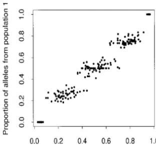
The case with admixture (Figure 2) appears to be correctly infer whether or not there was population
more difficult, even using many more loci. However, structure (K ⫽1 for data set 1 and K ⬎ 1 otherwise).
the clustering algorithm did manage to identify the In the case of data set 2A, which consisted of just 5
population structure appropriately and estimated the loci, there is not a clear estimate of K, as the posterior
ancestry of individuals with reasonable accuracy. Part probability is consistent with both the correct value, K⫽
of the reason that this problem is difficult is that it is 2, and also with K⫽3 or 4. However, when the number
hard to estimate the original allele frequencies (before of loci was increased to 15 (data set 2B), virtually all of
admixture) when almost all the individuals (7/8) are the posterior probability was on the correct number of
admixed. A more fundamental problem is that it is diffi-populations, K⫽2.
cult to get accurate estimates of q(i)for particular individ-Data set 3 was simulated under a more complicated
uals because (as can be seen from the y-axis of Figure model, where most individuals have mixed ancestry. In
2) for any given individual, the variance of how many this case, the population was formed by admixture of
Figure2.—Summary of the clustering results for simulated data set 3. Each point plots the estimated value of q(i)
1 (the proportion of ancestry in population 1) for a particular indi-vidual against the fraction of their alleles that were actually derived from population 1 (across the 60 loci genotyped). The five clusters (from left to right) are for individuals with 0, 1, . . . , 4 grandparents in population 1, respectively.
can be substantial (for intermediate q). This property means that even if the allele frequencies were known, it would still be necessary to use a considerable number
Figure3.—Neighbor-joining tree of individuals in the T. of loci to get accurate estimates of q for admixed individ- helleri data set. Each tip represents a single individual. C, M,
uals. N, and Y indicate the populations of origin (Chawia, Mbololo,
Ngangao, and Yale, respectively). Using the labels, it is possible Data from the Taita thrush: We now present results
to group the Chawia and Mbololo individuals into (somewhat) from applying our method to genotype data from an
distinct clusters, as marked. However, it would not be possible endangered bird species, the Taita thrush, Turdus helleri.
to identify these clusters if the population labels were not Individuals were sampled at four locations in southeast available. Individuals who appear to be misclassified are Kenya [Chawia (17 individuals), Ngangao (54), Mbololo marked *. One of these individuals [marked (*)] was also identified by our own algorithm as a possible migrant. The (80), and Yale (4)]. Each individual was genotyped at
tree was constructed using the program Neighbor included in seven microsatellite loci (Galbuseraet al. 2000).
Phylip (Felsenstein1993). The pairwise distance matrix was This data set is a useful test for our clustering method,
computed as follows (MountainandCavalli-Sforza1997). because the geographic samples are likely to represent For each pair of individuals, we added 1/L for each locus at distinct populations. These locations represent frag- which they had no alleles in common, 1/2L for each locus at which they had one allele in common (e.g., AA:AB or AB:AC), ments of indigenous cloud forest, separated from each
and 0 for each locus at which they had two alleles in common other by human settlements and cultivated areas. Yale,
(e.g., AA:AA or AB:AB), where L is the number of loci com-which is a very small fragment, is quite close to Ngangao.
pared. Extensive data on ringed and radio-tagged birds over a
3-year period indicate low migration rates (Galbusera
et al. 2000).
As discussed in background on clustering
meth-TABLE 2
ods, it is currently common to use distance-based
clus-tering methods to visualize genotype data of this kind. Summary statistics of variation within and between To permit a comparison between that type of approach geographic groups
and our own method, we begin by showing a
neighbor-Chawia Mbololo Ngangao Yale joining tree of the bird data (Figure 3). Inspection of
the tree reveals that the Chawia and Mbololo individuals
Chawia 5.1
represent (somewhat) distinct clusters. Several individu- Mbololo 7.1 5.6
als (marked by asterisks) appear to be classified with Ngangao 3.1 1.6 5.5
other groups. The four Yale individuals appear to fall Yale 1.9 2.3 0.1 6.0
within the Ngangao group [a view that is supported by
Diagonal, variance in repeat scores within groups; below summary statistics of divergence showing the Yale and diagonal, square of mean difference in repeat scores between Ngangao to be very closely related (Table 2)]. populations [(␦)2;GoldsteinandPollock1997, Equation
distance-based clustering methods. First, it would not be possible we obtained these results. Our clustering algorithm seems to have performed very well, with just a few indi-(in this case) to identify the appropriate clusters if the
labels were missing. Second, since the tree does not use viduals (labeled 1–4) falling somewhat outside the obvi-ous clusters. All of the points in the extreme corners a formal probability model, it is difficult to ask statistical
questions about features of the tree, for example: Are (some of which may be difficult to resolve on the pic-ture) are correctly assigned. The four Yale individuals the individuals marked with asterisks actually migrants,
or are they simply misclassified by chance? Is there evi- were assigned to the Ngangao cluster, consistent with the neighbor-joining tree and the (␦)2distances. We dence of population structure within the Ngangao group
(which appears from the tree to be quite diverse)? return to this data set inincorporating population informationto consider the question of whether the We now apply our clustering method to these data.
Choice of K, for Taita thrush data: To choose an individuals that seem not to cluster tightly with others sampled from the same location are the product of appropriate value of K for modeling the data, we ran a
series of independent runs of the Gibbs sampler at a migration.
Application to human data:The next data set, taken range of values of K. After running numerous
medium-length runs to investigate the behavior of the Gibbs fromJordeet al. (1995), includes data from 30 biallelic restriction site polymorphisms, genotyped in 72 Africans sampler (using the diagnostics described in Choice of K
for simulated data), we again chose to use a burn-in period (Sotho, Tsonga, Nguni, Biaka and Mbuti Pygmies, and San) and 90 Europeans (British and French).
of 30,000 iterations and to collect data for 106iterations.
We ran three to five independent simulations of this Application of our MCMC scheme with K ⫽ 2 indi-cates the presence of two very distinct clusters, corre-length for each K between 1 and 5 and found that the
independent runs produced highly consistent results. sponding to the Africans and Europeans in the sample (Figure 5). The model with K ⫽ 2 has vastly higher At K ⫽ 5, a run of 106 steps takes ⵑ70 min on our
desktop machine. posterior probability than the model with K⫽1.
Additional runs of the MCMC scheme with the mod-Using the approach described in Inference for the
num-ber of populations, we estimated Pr(X|K) for K ⫽ 1, els K ⫽ 3, 4, and 5 suggest that those models may be somewhat better than K⫽2. This may reflect the pres-2, . . . , 5 and corresponding values of Pr(K|X) for a
uniform prior on K ⫽ 1, 2, . . . , 5. (In fact, this data ence of population structure within the continental groupings, although in this case the additional popula-set contains a lot of information about K, so that
infer-ence is relatively robust to choice of prior on K, and tions do not form discrete clusters and so are difficult to interpret.
other priors, such as taking Pr(K) proportional to
Pois-son(1) for K⬎0, would give virtually indistinguishable Again it is interesting to contrast our clustering results with the neighbor-joining tree of these data (Figure 6). results.) From the estimates of Pr(K|X), shown in the
last column of Table 3, it is clear that the models with While our method finds it quite easy to separate the two continental groups into the correct clusters, it would K⫽1 or 2 are completely insufficient to model the data
and that the model with K ⫽ 3 is substantially better not be possible to use the neighbor-joining tree to detect distinct clusters if the labels were not present. The data than models with larger K. Given these results, we now
focus our subsequent analysis on the model with three set of Jorde also contains a set of individuals of Asian origin (which are more closely related to Europeans populations.
Clustering results for Taita thrush data: Figure 4 than are Africans). Neither the neighbor-joining method nor our method differentiates between the Eu-shows a plot of the clustering results for the individuals
in the sample, assuming that there are three populations ropeans and Asians with great accuracy using this data set.
(as inferred above). We did not use (and indeed, did not know) the sampling locations of individuals when
INCORPORATING POPULATION INFORMATION
TABLE 3 The results presented so far have focused on testing
Inferring the value ofK, the number of populations, how well our method works. We now turn our attention
for theT. helleridata to some further applications of this method.
Our clustering results (Figure 4) confirm that the K log P(X|K) P(K|X) three main geographic groupings in the thrush data set (Chawia, Mbololo, and Ngangao) represent three
1 ⫺3144 ⵑ0
genetically distinct populations. The geographic labels
2 ⫺2769 ⵑ0
3 ⫺2678 0.993 correspond very closely to the genetic clustering in all 4 ⫺2683 0.007 but a handful of cases (1–4 in Figure 4). Individual 2 5 ⫺2688 0.00005 is also identified as a possible outlier on the neighbor-joining tree (Figure 3). Given this, it is natural to ask The values in the last column assume a uniform prior for
de-Figure4.—Summary of the clustering results for the T. helleri data assuming three populations. Each point shows the mean estimated ancestry for an individual in the sample. For a given individual, the values of the three coefficients in the ancestry vector q(i) are given by the distances to each of the three sides of the equilateral triangle. After the clustering was performed, the points were la-beled according to sampling location. Numbers 1–4 are individuals who appear to be possible outliers (see text). For clarity, the four Yale indi-viduals (who fall into the Ngangao cluster) are not plotted. We were not told the sampling loca-tions of individuals until after we obtained these results.
scendants of recent immigrants) from other popula- whose genetic makeup suggests they were misclassified. Thus, while we speak of “immigrants” and “immigrant tions. For example, given the genetic data, how probable
is it that individual 1 is actually an immigrant from ancestry,” in some contexts these terms may relate to something other than changes in physical location. Chawia?
To answer this sort of question, we need to extend Provided that geographic labels usually correspond to population membership, using the geographic infor-our algorithm to incorporate the geographic labels. By
doing this, we break the symmetry of the labels, and we can ask specifically whether a particular individual is a migrant from Chawia (say). In essence our approach (described more formally in the next section) is to as-sume that each individual originated, with high proba-bility, in the geographical region in which it was sam-pled, but to allow some small probability that it is an immigrant (or has immigrant ancestry). Note that this model is also suitable for situations in which individuals are classified according to some characteristic other than sampling location (physical appearance, for exam-ple). “Immigrants” in this situation would be individuals
Figure5.—Summary of the clustering results for the data set of Africans and Europeans taken fromJordeet al. (1995).
For each individual, we computed the mean value of q(i) 1 (the
Figure6.—Neighbor-joining tree of individuals in the data proportion of ancestry in population 1), over a single run of
the Gibbs sampler. The dashed line is a histogram of mean set ofJordeet al. (1995). Each tip represents a single
individ-ual. A and E indicate that individuals were African or Euro-values of q(i)
1 for individuals of European origin; the solid line
mation will clearly improve our accuracy at assigning 2t
(K⫺1)RG T⫽0 2T
, (17)
individuals to clusters; it will also improve our estimates of P, thus also giving us greater precision in assignment
where t 苸 {0, . . . , G }. As before, q(i)
l ⱖ 0 for l 苸
of individuals who do not have geographic information.
{1, . . . , K }, andRq(i)
l ⫽1.
However, in practice we suggest that before making use
Again, we can sample from Pr(Q|X) using Algorithm of such information, users of our method should first
2. In this case, however, since there are a small number cluster the data without using the geographic labels, to
of possible values of q(i), we update q(i)by sampling di-check that the genetically defined clusters do in fact
rectly from the posterior probability of q(i)|X,P, rather agree with geographic labels. We return to this issue in
than conditional on Z. thediscussion.
Note that in this framework, it is easy to include indi-RannalaandMountain(1997) also considered the
viduals for whom there is no geographic information problem of detecting immigrants and individuals with
by using the same prior and update steps as before recent immigrant ancestors, taking a somewhat similar
(Equations 7 and A10). approach to that used here. However, rather than
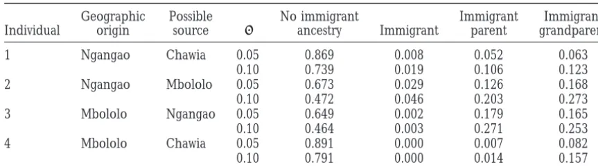
con-Testing for migrants in the Taita thrush data: To apply sidering all individuals simultaneously, as we do here,
our method, we must first specify a value for. In this they test each individual in the sample, one at a time,
case, based on mark-release-recapture data from these as a possible immigrant, assuming that all the other
populations (Galbuseraet al. 2000), migration seems individuals are not immigrants. This approach will have
relatively rare, and so is likely to be small. We per-reduced power to detect immigrants if the sample
con-formed analyses for ⫽0.05 and ⫽0.1; a summary tains several immigrants from one population to
an-of the results is shown in Table 4. Individuals 2 and 3 other. In contrast, our approach can cope well with this
have moderate posterior probabilities of having migrant kind of situation.
ancestry, but these probabilities are perhaps smaller Model with prior population information:To
incor-than might be expected from examining Figure 4. This porate geographic information, we use the following
is due to a combination of the low prior probability for model. Our primary goal is to identify individuals who
migration (from the mark-release-recapture data) and, are immigrants, or who have recent immigrant ancestry,
perhaps more importantly, the fact that there is a limited in the last G generations, say, where G⫽0 is the present
amount of information in seven loci, so that the uncer-generation. [In practice there will only be substantial
tainty associated with the position of the points marked power to detect immigration for small G; cf. Rannala
1, 2, 3, and 4 in Figure 4 may be quite large. A more andMountain(1997).]
definite conclusion could be obtained by typing more First, we code each of the geographic locations by a
loci. (unique) integer between 1 and K, where K would
usu-It is interesting to note that our conclusions here ally be set equal to the number of locations. Using this
differ from those obtained on this data set using the coding, let g(i)represent the geographic sampling
loca-package IMMANC (Rannala and Mountain 1997). tion of individual i. Now, let be the probability that
IMMANC indicates that three individuals (1, 2, and 3 an individual is an immigrant to population g(i)or has an
here) show significant evidence of immigrant ancestry immigrant ancestor in the last G generations. Otherwise,
at the 0.01 significance level (Galbuseraet al. 2000). with probability 1 ⫺ , the individual is considered to
However, IMMANC does not make a multiple compari-be purely from population g(i). While in principle one
sons correction; such a correction would bring those could place a prior on and learn about it from the
results into line with ours. data as part of the MCMC scheme, in our current
imple-We anticipate that our method might also be applied mentation the user must specify a fixed value for; we
in situations where there is little data to help make an give some guidelines in the next section.
informed choice of . In such situations we suggest Assuming that migration is rare, we can use the
ap-analyzing the data using several different values of, to proximation that each individual has at most one
immi-see whether the conclusions are robust to choice of. grant ancestor in the last G generations (where G is
The range of sensible values for will depend on the suitably small). Then, assuming a constant migration
context, but typically we suggest values in the range rate, the probability of an immigrant ancestor in
genera-0.001–0.1 might be appropriate. Sensitivity to choice of tion t (0 ⱕ t ⱕ G) is proportional to 2t, where t ⫽ 0
indicates that the amount of information in the data indicates that the individual migrated in the present
is insufficient to draw strong conclusions. generation. Thus, we set the prior on q(i)to be
q(i)g(i)⫽1, qk(i)⫽0 (k⬆g(i)) (15)
DISCUSSION with probability 1 ⫺ and
We have described a method for using multilocus q(i)g(i)⫽1⫺2⫺t, q(i)j ⫽2⫺t, q(i)k ⫽0 (k⬆g(i), j) (16)
TABLE 4
Testing whether particular individuals are immigrants or have recent immigrant ancestors
Geographic Possible No immigrant Immigrant Immigrant Individual origin source ancestry Immigrant parent grandparent
1 Ngangao Chawia 0.05 0.869 0.008 0.052 0.063
0.10 0.739 0.019 0.106 0.123
2 Ngangao Mbololo 0.05 0.673 0.029 0.126 0.168
0.10 0.472 0.046 0.203 0.273
3 Mbololo Ngangao 0.05 0.649 0.002 0.179 0.165
0.10 0.464 0.003 0.271 0.253
4 Mbololo Chawia 0.05 0.891 0.000 0.007 0.082
0.10 0.791 0.000 0.014 0.157
The individuals are labeled as shown in Figure 4. “No immigrant ancestry” gives the probability that the ancestry of each individual is exclusively in the geographic origin population; the following columns show the probabilities that each individual has the given amount of ancestry in the possible source population. The rows do not add to 1 because there are small probabilities associated with individuals having ancestry in the third population.
Our method also provides a novel approach to testing preclassified individuals are used to estimate allele fre-quencies (cf.Smouseet al. 1990).
for the presence of population structure (K⬎ 1).
Our examples demonstrate that the method can accu- Another type of application where the geographic information might be of value is in evolutionary studies rately cluster individuals into their appropriate
popula-tions, even using only a modest number of loci. In prac- of population relationships. Such analyses frequently make use of summary statistics based on population tice, the accuracy of the assignments depends on a
number of factors, including the number of individuals allele frequencies [e.g., FST and (␦)2]. In situations where the population allele frequencies might be af-(which affects the accuracy of the estimate for P), the
number of loci (which affects the accuracy of the esti- fected by recent immigration or where population classi-fications are unclear, such summary statistics could be mate for Q), the amount of admixture, and the extent
of allele-frequency differences among populations. calculated directly from the population allele frequen-cies P estimated by the Gibbs sampler.
We anticipate that our method will be useful for
iden-tifying populations and assigning individuals in situa- There are several ways in which the basic model that we have described here might be modified to produce tions where there is little information about population
structure. It should also be useful in problems where better performance in particular cases. For example, in models and methodsandapplications to data we cryptic population structure is a concern, as a way of
identifying subpopulations. Even in situations where assumed relatively noninformative priors for q. How-ever, in some situations, there might be quite a bit of there is nongenetic information that can be used to
define populations, it may be useful to use the approach information about likely values of q, and the estimation procedure could be improved by using that informa-developed here to ensure that populations defined on
an extrinsic basis reflect the underlying genetic struc- tion. For example, in estimating admixture proportions for African Americans, it would be possible to improve ture.
As described inincorporating population infor- the estimation procedure by making use of existing in-formation about the extent of European admixture mationwe have also developed a framework that makes
it possible to combine genetic information with prior (e.g., Parraet al. 1998).
A second way in which the basic model can be modi-information about the geographic sampling location of
individuals. Besides being used to detect migrants, this fied involves changing the way in which the allele fre-quencies P are estimated. Throughout this article, we could also be used in situations where there is strong
prior population information for some individuals, but have assumed that the allele frequencies in different populations are uncorrelated with one another. This is not for others. For example, in hybrid zones it may be
possible to identify some individuals who do not have a convenient approximation for populations that are not extremely closely related and, as we have seen, can mixed ancestry and then to estimate q for the rest (M.
Beaumont, D. Gotelli, E. M. Barett, A. C. Kitch- produce accurate clustering. However, loosely speaking, the model of uncorrelated allele frequencies says that ener, M. J. Daniels, J. K. PritchardandM. W.
Bru-ford, unpublished results). The advantage of using a we do not normally expect to see populations with very similar allele frequencies. This property has the result clustering approach in such cases is that it makes the
which we have implemented in our software package, enough to make the population act as a single unstruc-tured population.
is to permit allele frequencies to be correlated across
In summary, we find that the method described here populations (appendix,Model with correlated allele
frequen-can produce highly accurate clustering and sensible cies). In a series of additional simulations, we have found
choices of K, both for simulated data and for real data that this allows us to perform accurate assignments of
from humans and from the Taita thrush. In the latter individuals in very closely related populations, though
example, we find it particularly encouraging that using possibly at the cost of making us likely to overestimate K.
a relatively small number of loci (seven) we can detect Our basic model might also be modified to allow for
a very strong signal of population structure and assign linkage among marker loci. Normally, we would not
individuals appropriately. expect to see linkage disequilibrium within
subpopula-The algorithms described in this article have been tions, except between markers that are extremely close
implemented in a computer software package structure, together. This means that in situations where there is
which is available at http://www.stats.ox.ac.uk/ⵑpritch/ little admixture, our assumption of independence
home.html. among loci will be quite accurate. However, we might
expect to see strong correlations among linked loci We thank Peter Galbusera and Lynn Jorde for allowing us to use their data, Augie Kong for a helpful discussion, Daniel Falush for
when there is recent admixture. This occurs because
suggesting comparison with neighbor-joining trees, Steve Brooks and
an individual who is admixed will inherit large
chromo-Trevor Sweeting for helpful discussions on inferring K, and Eric
An-somal segments from one population or another. Thus,
derson for his extensive comments on an earlier version of the
manu-when the map order of marker loci is known, it should script. This work was supported by National Institutes of Health grant be possible to improve the accuracy of the estimation for GM19634 and by a Hitchings-Elion fellowship from Burroughs-Well-come Fund to J.K.P., by a grant from the University of Oxford and
such individuals by modeling the inheritance of these
a Wellcome Trust Fellowship (057416) to M.S., and by grants GR/
segments.
M14197 and 43/MMI09788, from the Engineering and Physical
Sci-In this article we have devoted considerable attention
ences Research Council and Biotechnology and Biological Sciences
to the problem of inferring K. This is an important Research Council, respectively, to P.D. The work was initiated while practical problem from the standpoint of model choice. the authors were resident at the Isaac Newton Institute for
Mathemati-cal Sciences, Cambridge, UK.
We need to have some way of deciding which clustering model is most appropriate for interpreting the data. However, we stress that care should be taken in the
interpretation of the inferred value of K. To begin with, LITERATURE CITED due to the very high dimensionality of the parameter
Balding, D. J.,andR. A. Nichols,1994 DNA profile match
proba-space, we found it difficult to obtain reliable estimates bility calculations: how to allow for population stratification, relat-of Pr(X | K) and have chosen to use a fairly ad hoc edness, database selection and single bands. Forensic Sci. Int.
64:125–140.
procedure that we have found gives sensible results in
Balding, D. J.,andR. A. Nichols,1995 A method for quantifying
practice. Second, it has been observed that in Bayesian differentiation between populations at multi-allelic loci and its model-based clustering, the posterior distribution of K implications for investigating identity and paternity. Genetica 96:
3–12.
tends to be quite dependent on the priors and modeling
Bowcock, A. M., A. Ruiz-Linares, J. Tomfohrde, E. Minch, J. Kidd
assumptions, even though estimates of the other param- et al., 1994 High resolution of human evolutionary trees with eters (e.g., P and Q here) may be reasonably robust polymorphic microsatellites. Nature 368: 455–457.
Cavalli-Sforza, L. L., P. MenozziandA. Piazza,1994 The History (see Richardson and Green 1997; Stephens 2000a,
and Geography of Human Genes. Princeton University Press,
for example). Princeton, NJ.
Chib, S.,1995 Marginal likelihood from the Gibbs output. J. Am.
There are also biological reasons to be careful
inter-Stat. Assoc. 90: 1313–1321.
preting K. The population model that we have adopted
Chib, S.,andE. Greenberg,1995 Understanding the
Metropolis-here is obviously an idealization. We anticipate that it Hastings algorithm. Am. Stat. 49: 327–335.
will be flexible enough to permit appropriate clustering Davies, N., F. X. VillablancaandG. K. Roderick,1999 Deter-mining the source of individuals: multilocus genotyping in
for a wide range of population structures. However, as
nonequilibrium population genetics. TREE 14: 17–21.
we pointed out in our discussion of data set 3 (Choice DiCiccio, T., R. Kass, A. RafteryandL. Wasserman,1997 Com-of K for simulated data), clusters may not necessarily corre- puting Bayes factors by posterior simulation and asymptotic
ap-proximations. J. Am. Stat. Assoc. 92: 903–915.
spond to “real” populations. As another example,
imag-Ewens, W. J.,andR. S. Spielman,1995 The
transmission/disequilib-ine a species that lives on a continuous plane, but has rium test: history, subdivision, and admixture. Am. J. Hum. Genet. low dispersal rates, so that allele frequencies vary contin- 57:455–464.
Felsenstein, J.,1993 PHYLIP (phylogeny inference package)
ver-uously across the plane. If we sample at K distinct
loca-sion 3.5c. Technical report, Department of Genetics, University
tions, we might infer the presence of K clusters, but the of Washington, Seattle.
inferred number K is not biologically interesting, as it Foreman, L., A. SmithandI. Evett,1997 Bayesian analysis of DNA profiling data in forensic identification applications. J. R. Stat.
was determined purely by the sampling scheme. All that
Soc. A 160: 429–469.
can usefully be said in such a situation is that the migra- Galbusera, P., L. Lens, E. Waiyaki, T. SchenckandE. Mattysen,
2000 Effective population size and gene flow in the globally,
critically endangered Taita thrush, Turdus helleri. Conserv. Genet. stationary distribution (). This is often surprisingly (in press).
straightforward using standard methods devised for this
Gilks, W. R., S. RichardsonandD. J. Spiegelhalter,1996a
Intro-ducing Markov chain Monte Carlo, pp. 1–19 in Markov Chain purpose, such as the Metropolis-Hastings algorithm
Monte Carlo in Practice, edited by W. R. Gilks, S. Richardson (e.g.,ChibandGreenberg1995) and Gibbs sampling
andD. J. Spiegelhalter.Chapman & Hall, London.
(e.g., Gilks et al. 1996a), which we describe in more
Gilks, W. R., S. RichardsonandD. J. Spiegelhalter (Editors),
1996b Markov Chain Monte Carlo in Practice. Chapman & Hall, detail below. Intuitively, if the Markov chain (0), (1),
London. (2), . . . has stationary distribution (), then (m) will
Goldstein, D. B.,andD. Pollock,1997 Launching microsatellites:
be approximately distributed as() provided m is
suf-a review of mutsuf-ation processes suf-and methods of phylogenetic
inference. J. Hered. 88: 335–342. ficiently large. This can be formalized and shown to be
Green, P. J.,1995 Reversible jump Markov chain Monte Carlo com- true provided the Markov chain satisfies certain techni-putation and Bayesian model determination. Biometrika 82: 711–
cal conditions (ergodicity) that hold for the Markov
732.
Hudson, R. R.,1990 Gene genealogies and the coalescent process, chains considered in this article. Furthermore, for
suffi-pp. 1–44 in Oxford Surveys in Evolutionary Biology, Vol. 7, edited ciently large c,(m),(m⫹c),(m⫹2c), . . . will be reasonably
by D. Futuymaand J. Antonovics. Oxford University Press,
independent samples from(). The value of m used
Oxford.
Jorde, L. B., M. J. Bamshad, W. S. Watkins, R. Zenger, A. E. Fraley is often referred to as the burn-in period of the chain; et al., 1995 Origins and affinities of modern humans: a compari- c is often referred to as the thinning interval.
son of mitochondrial and nuclear genetic data. Am. J. Hum.
In general it is very difficult to know how large m
Genet. 57: 523–538.
Mountain, J. L.,andL. L. Cavalli-Sforza,1997 Multilocus geno- and c should be. The values required to obtain reliable
types, a tree of individuals, and human evolutionary history. Am. results depend heavily on the amount of correlation
J. Hum. Genet. 61: 705–718.
between successive states of the Markov chain. If
succes-Paetkau, D., W. Calvert, I. StirlingandC. Strobeck,1995
Mi-crosatellite analysis of population structure in Canadian polar sive states are relatively uncorrelated (that is, if the chain
bears. Mol. Ecol. 4: 347–354. moves quickly between reasonably different values of
Parra, E. J., A. Marcini, J. Akey, J. Martinson, M. A. Batzeret al.,
), then the chain is said to mix well, and relatively small
1998 Estimating African American admixture proportions by
use of population-specific alleles. Am. J. Hum. Genet. 63: 1839– values of m and c will suffice. Conversely, if the chain
1851.
mixes badly (sometimes known as being sticky, as the
Pritchard, J. K.,andN. A. Rosenberg,1999 Use of unlinked
ge-chain will tend to get stuck moving among very similar
netic markers to detect population stratification in association
studies. Am. J. Hum. Genet. 65: 220–228. values of), then very large values of m and c will be
Raftery, A. E.,1996 Hypothesis testing and model selection, pp.
required, possibly rendering the method impracticable.
163–188 in Markov Chain Monte Carlo in Practice, edited byW. R.
One strategy for investigating whether m and c are
suffi-Gilks, S. Richardson andD. J. Spiegelhalter.Chapman &
Hall, London. ciently large, and the strategy we adopt here, is to
simu-Rannala, B.,andJ. L. Mountain,1997 Detecting immigration by
late several realizations of the Markov chain, each
start-using multilocus genotypes. Proc. Natl. Acad. Sci. USA 94: 9197–
ing from a different value of (0). If m and c are
9201.
Richardson, S., andP. J. Green, 1997 On Bayesian analysis of sufficiently large, then the results obtained should be mixtures with an unknown number of components. J. R. Stat.
independent of(0)and should therefore be similar for
Soc. Ser. B 59: 731–792.
the different runs. Substantial differences among the
Roeder, K., M. Escobar, J. B. KadaneandI. Balazs,1998
Measur-ing heterogeneity in forensic databases usMeasur-ing hierarchical Bayes results obtained for the different runs indicate that m
models. Biometrika 85: 269–287.
and c are too small. It is then necessary either to increase
Smouse, P. E., R. S. WaplesandJ. A. Tworek, 1990 A genetic
m and c or (if this makes the method computationally
mixture analysis for use with incomplete source population-data.
Can. J. Fish. Aquat. Sci. 47: 620–634. infeasible) to construct a Markov chain with better
mix-Spiegelhalter, D. J., N. G. BestandB. P. Carlin,1999 Bayesian
ing properties. In the examples presented in this article
deviance, the effective number of parameters, and the
compari-son of arbitrarily complex models. Available from http:// we have chosen c⫽ 1.
www.mrc-bsu.cam.ac.uk/publications/preslid.shtml. Gibbs sampling is a method of constructing a Markov
Stephens, M.,2000a Bayesian analysis of mixtures with an unknown
chain with stationary distribution (), which has
number of components—an alternative to reversible jump
meth-ods. Ann. Stat. (in press). proved particularly useful for clustering problems.
Sup-Stephens, M.,2000b Dealing with label-switching in mixture mod- pose that may be partitioned into ⫽(
1, . . . ,r),
els. J. R. Stat. Soc. Ser. B (in press).
and that although it is not possible to simulate from
Communicating editor:M. K. Uyenoyama () directly, it is possible to simulate a random value
of i directly from the full conditional distribution
(i |1,2, . . . ,i⫺1,i⫹1, . . . ,r) for i⫽ 1, 2, . . . ,
APPENDIX r. Then the following algorithm may be used to simulate
a Markov chain with stationary distribution(): MCMC methods and Gibbs sampling:
Algorithm A1: Starting with initial values (0) ⫽ MCMC methods are extremely useful for obtaining ((0)
1 , . . . , (0)r ), iterate the following steps for m ⫽ 1,
(approximate) samples from a probability distribution, 2, . . . .
(), say, which cannot be simulated from directly [in
Step 1. Sample(m)
1 from(1|2(m⫺1),(m⫺1)3 , . . . ,(m⫺1)r ).
our case ⫽(Z, P, Q) and()⫽Pr(Z, P, Q|X)]. The
idea is to construct a Markov chain(0),(1),(2), . . . with Step 2. Sample(m)