ABSTRACT
WU, XING. Scalable Communication Tracing for Performance Analysis of Parallel Applications. (Under the direction of Frank Mueller.)
Performance analysis and prediction for parallel applications is important for the design and development of scientific applications, and for the construction and procurement of high-performance computing (HPC) systems. As one of the most important approaches, application tracing is widely used for this purpose for being able to provide the computation and commu-nication details of an application. Recent progress in commucommu-nication tracing has tremendously improved the scalability of tracing tools and reduced the size of the trace file, and thereby opened up novel opportunities for trace-based performance analysis for parallel applications.
This work focuses on domain-specific trace compression methodology and puts forth fun-damentally new approaches to improve the communication tracing techniques. Facilitated by the advances in this area, novel algorithms are further designed to address the hard problem of performance analysis, prediction, and benchmarking at scale. Specifically, this work makes the following contributions:
1. This work contributes ScalaExtrap, a fundamentally novel performance modeling scheme and tool. With ScalaExtrap, we synthetically generate the application trace for large numbers of MPI tasks by extrapolating from a set of smaller traces. We devise an innova-tive approach for topology extrapolation of SPMD (Single Program Multiple Data) codes with stencil or mesh communication. The extrapolated trace can subsequently be used for trace-based simulation, visualization, and detection of communication inefficiencies and scalability limitations at scale.
2. This work contributes novel methods to automatically generate highly portable and cus-tomizable communication benchmarks from HPC applications. We utilize ScalaTrace to collect selected aspects of the run-time behavior of HPC applications. We then generate portable and easy-to-read benchmarks with identical run-time behavior from the collected traces with C and the rich-featuredcoNCePTuaLnetwork benchmarking language. Be-cause our approach supports code obfuscation, it is particularly valuable for proprietary, export-controlled, or classified applications.
trace compression for applications with iteration-specific program behavior and diverging parallel control flow. A fully distributed replay tool for probabilistic traces is also de-veloped for the reproduction of the computation performance of the original application. The respective design has been implemented in ScalaTrace 2, the next generation of the ScalaTrace tracing infrastructure.
c
Copyright 2013 by Xing Wu
Scalable Communication Tracing for Performance Analysis of Parallel Applications
by Xing Wu
A dissertation submitted to the Graduate Faculty of North Carolina State University
in partial fulfillment of the requirements for the Degree of
Doctor of Philosophy
Computer Science
Raleigh, North Carolina
2013
APPROVED BY:
Xiaosong Ma Yan Solihin
Xiaohui Helen Gu Scott Pakin
Frank Mueller
DEDICATION
BIOGRAPHY
ACKNOWLEDGEMENTS
All of a sudden, when I finally had the opportunity to write down my acknowledgement for this dissertation, I came to realize that it is almost the end of my Ph.D journey. In retrospect, the memories of so many first times are still fresh: the first time fighting a twelve-hour jet lag in an operating systems class that I could not really understand, the first time sitting in Room 3266 struggling to comprehend a complication called ScalaTrace, the first time receiving a rejection for an ambitious paper submission, the first time standing behind a podium giving a conference presentation, the first time working in a national lab at an once secret location, the first time passing a job interview and getting a position in a dream company ... . Throughout the journey, there were disappointment, depression, frustration, and suffering, but there were also excitement, cheerfulness, brilliance, and most importantly, achievements, which are never possible without the encouragement, guidance, and support from the people to whom I shall show my gratitude.
Firstly, I would like to thank my family. I thank my parents for supporting their only child to pursue a graduate degree in a country that is thousands of miles away. I thank my wonderful wife, Yi, for enduring the loneliness of being geographically apart for ten years, and for all the unselfish sacrifice thereafter. Their constant understanding and tremendous support encouraged me to move on.
Secondly, I would like to thank my advisor Dr. Frank Mueller, for his patience and encour-agement to a beginner in the first few years, and for his professional guidance and invaluable advice throughout my studies. His wisdom, expertise, and insightful thoughts motivated me and inspired my research. I would also thank Dr. Xiaosong Ma, Dr. Xiaohui Gu, Dr. Yan Solihin, and Dr. Scott Pakin for serving on my advisory committee and giving me invaluable suggestions on my dissertation. Particularly, I would like to give special thanks to Dr. Scott Pakin for being my mentor during my internship at Los Alamos National Laboratory and being my collaborator of one of my papers. Since we worked together, he has given me substantial help on my research.
TABLE OF CONTENTS
List of Tables . . . vii
List of Figures . . . .viii
Chapter 1 Introduction . . . 1
1.1 Background . . . 1
1.1.1 The Recent History of Supercomputers . . . 1
1.1.2 Application Trace for Performance Analysis and Prediction . . . 2
1.1.3 ScalaTrace . . . 3
1.2 Hypothesis . . . 4
1.3 Contributions . . . 4
1.3.1 Contributions . . . 4
1.3.2 Assumptions and Scope . . . 6
1.4 Organization . . . 6
Chapter 2 An Overview of ScalaTrace . . . 8
2.1 Intra-node and Inter-node Compression . . . 8
2.2 ScalaTrace Encoding Schemes . . . 9
2.3 Preserving Time in Communication Traces . . . 10
2.4 ScalaReplay . . . 11
Chapter 3 ScalaExtrap: Trace Extrapolation for SPMD Programs . . . 12
3.1 Introduction . . . 12
3.2 Communication Extrapolation . . . 14
3.2.1 Topology Identification . . . 15
3.2.2 Matching MPI Events for Extrapolation . . . 17
3.2.3 Extrapolation of MPI Events . . . 20
3.2.4 Lossy Extrapolation . . . 23
3.2.5 Extrapolation of Timing Information . . . 25
3.3 Experimental Framework . . . 26
3.4 Experimental Results . . . 27
3.4.1 Correctness of Communication Trace Extrapolation . . . 28
3.4.2 Accuracy of Extrapolated Timings: Timed Replay . . . 30
3.4.3 Lossy Extrapolation . . . 35
3.5 Application of the Extrapolated Trace . . . 36
3.5.1 Extrapolated Trace for Code Generation . . . 37
3.5.2 Extrapolated Trace for Performance Experiments . . . 37
3.6 Related Work . . . 39
Chapter 4 Automatic Generation of Parallel Benchmarks from Applications . 44
4.1 Introduction . . . 44
4.2 Related Work . . . 47
4.3 coNCePTuaL . . . 49
4.4 Benchmark Generation . . . 50
4.4.1 Overview . . . 50
4.4.2 Engineering Details . . . 52
4.4.3 Combining Per-Node Collectives . . . 53
4.4.4 Eliminating Nondeterminism . . . 55
4.4.5 The Generation of Scalable Benchmarks . . . 59
4.4.6 Sources of Performance Inaccuracy . . . 61
4.5 Evaluation . . . 61
4.5.1 Experimental Framework . . . 61
4.5.2 Communication Correctness . . . 62
4.5.3 Accuracy of Generated Timings . . . 63
4.5.4 Correctness and Timing Accuracy of Generated Scalable Benchmarks . . 63
4.5.5 Applications of the Benchmark Generator . . . 66
4.6 Summary . . . 72
Chapter 5 ScalaTrace 2 . . . 74
5.1 Introduction . . . 74
5.2 Communication Trace Compression and Replay . . . 76
5.2.1 Elastic Data Element Representation . . . 76
5.2.2 Compressing Partially Matching Loops . . . 77
5.2.3 Approximate Stack Signature Matching . . . 81
5.2.4 Loop Agnostic Inter-node Compression . . . 83
5.2.5 Customizable Instrumentation . . . 85
5.2.6 Replaying Non-deterministic Trace . . . 86
5.3 Evaluation . . . 88
5.3.1 Trace File Size . . . 89
5.3.2 Probabilistic Replay Time Accuracy . . . 92
5.4 Related Work . . . 94
5.5 Summary . . . 96
Chapter 6 Future Work . . . 97
6.1 Customizable Instrumentation . . . 97
6.2 A Versatile Tracing Framework with Tunable Precision . . . 98
6.3 Scalable Numerical Data Analysis Techniques . . . 99
Chapter 7 Conclusion . . . .100
LIST OF TABLES
LIST OF FIGURES
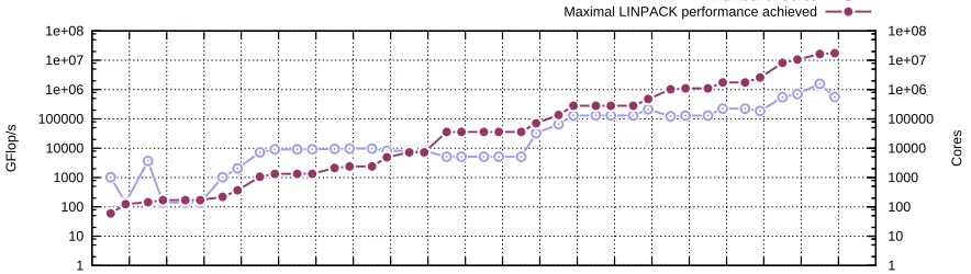
Figure 1.1 Performance Development of Supercomputers Since June 1993 . . . 2
Figure 2.1 Sample Stencil Code for RSD and PRSD Generation . . . 9
Figure 2.2 Ranklist Representation for Communication Group . . . 10
Figure 3.1 Topology Detection . . . 16
Figure 3.2 Boundary Size Calculation . . . 16
Figure 3.3 Inter-node Compression and the Positions of Communication Groups . . . 18
Figure 3.4 Generic Representation of Communication Endpoints . . . 21
Figure 3.5 Set of Equations for Communication Endpoint Extrapolation . . . 21
Figure 3.6 Distribution of Communication Groups of a 2D Stencil Code . . . 22
Figure 3.7 A Simple Trace Snippet and the Generated Finite-state Machine . . . 24
Figure 3.8 CG Communication Topology . . . 27
Figure 3.9 Correctness of Trace Extrapolation and Replay . . . 28
Figure 3.10 Replay Time Accuracy for Strong Scaling Benchmarks . . . 31
Figure 3.11 Replay Time Accuracy for Weak Scaling Benchmarks . . . 34
Figure 3.12 Timing Accuracy of Lossy Extrapolation of Weak Scaling MG . . . 36
Figure 3.13 Timing Accuracy for the Extrapolated Benchmarks . . . 38
Figure 3.14 The Impact of Computational Speedup on the Overall Performance . . . . 39
Figure 4.1 Benchmark Generation System . . . 45
Figure 4.2 Pseudo MPI Code for 1D Torus Communication . . . 49
Figure 4.3 coNCePTuaL Code for the Pseudo MPI Code in Figure 4.2 . . . 50
Figure 4.4 Combining Collectives Across Separate Source-code Statements . . . 53
Figure 4.5 Operation of Algorithm 2 . . . 56
Figure 4.6 Potential Deadlock . . . 57
Figure 4.7 Communication Pattern of a 2D Stencil Code . . . 60
Figure 4.8 Time Accuracy for Generated Benchmarks . . . 64
Figure 4.9 Timing Accuracy of the ScalablecoNCePTuaLBenchmarks . . . 65
Figure 4.10 Communication Performance of BT . . . 67
Figure 4.11 Impact of Communication Performance on BT . . . 68
Figure 4.12 CompletecoNCePTuaLCode for NPB FT (Class C) of 256 MPI Tasks 69 Figure 4.13 Performance of All-to-all Implementations for FT . . . 70
Figure 4.14 Cross-platform Prediction . . . 72
Figure 5.1 Loop with Iteration-specific Behavior . . . 78
Figure 5.2 Loop with Trailing Iterations . . . 80
Figure 5.3 The Simplified NPB BT Code . . . 83
Figure 5.4 Code Needs Loop Agnostic Inter-node Compression . . . 84
Figure 5.5 Final Trace of the Code in Figure 5.4 . . . 85
Figure 5.6 Trace Needs Multiple Context Pointers for Replay . . . 87
Chapter 1
Introduction
1.1
Background
1.1.1 The Recent History of Supercomputers
Processor counts and Flops (FLoating-point Operations Per Second) in modern supercomputers are rising exponentially. Back in June 1993, when the first Top500 list [1] was announced, the CM-5/1024, the world’s fastest supercomputer from Los Alamos National Laboratory at the time had only 1,024 cores and a maximal LINPACK [21] performance (Rmax) of 59.7 GFlops.
Four years later, in June 1997, the world’s first teraflop supercomputer, ASCI Red from Sandia National Laboratories with 7,264 cores and anRmax of 1,068 GFlops, became the number one
system in the world. In June 2008, the Roadrunner system at Los Alamos National Labora-tory with 122,400 cores and anRmax of 1,026.00 TFlops brought the global high performance
computing community into the era of petascale for the first time. As of the publication of the latest Top500 list (November 2012), all of the top 20 systems have achieved petaflop/s perfor-mance. Titan, the Cray XK7 supercomputer at the Oak Ridge National Laboratory capable of performing more than 17 quadrillion calculations per second (PFlops), currently occupies the first place in the list. It (together with the June 2012 champion, Sequoia BlueGene/Q with 1,572,864 cores and anRmax of 16.3 PFlops at the Lawrence Livermore National Laboratory)
1 10 100 1000 10000 100000 1e+06 1e+07 1e+08
1993 1994 1995 1996 1997 1998 1999 2000 2001 2002 2003 2004 2005 2006 2007 2008 2009 2010 2011 2012 2013 2014 1 10 100 1000 10000 100000 1e+06 1e+07 1e+08
GFlop/s Cores
Number of Cores Maximal LINPACK performance achieved
Figure 1.1: Performance Development of Supercomputers Since June 1993
1.1.2 Application Trace for Performance Analysis and Prediction
Performance analysis and prediction for scientific applications is important for assessing po-tential application performance and HPC systems procurement. However, as supercomputers progress in scale and capability toward exascale levels, characterization of communication be-havior and its impact on the overall application performance is becoming increasingly difficult due to the application size and system complexity.
Performance modeling is an important approach to predict application behavior. Generally, this approach takes a number of machine and application parameters as input. It utilizes a set of formulae to assess the performance of an application when it is executed on a partic-ular architecture and at a certain scale. Nonetheless, measuring the system and application performance parameters is non-trivial given the complexity of supercomputers and large-scale scientific applications. In addition, this approach provides only the predicted overall statistics for an application. Without detailed application runtime information, neither more sophisti-cated static analysis nor post-mortem performance debugging is possible.
Profiling is another widely used method for performance analysis and debugging of scientific codes that utilize MPI-style message passing [34]. Through binary instrumentation or utilizing the MPI profiling layer, profiling tools, such as mpiP [75], are able to gather runtime information such as the execution times of the functions and the message volume exchanged in the network. Nevertheless, as a light-weighted approach, profiling provides only the aggregated statistics of an application. Without the structural and temporal ordering of events and the information about each communication event and each computation region, in-depth and fine-grained performance analysis can hardly be done.
wrap-per functions for the actual MPI functions. By intercepting MPI calls at the profiling interface, the MPI profiling system can record useful information including the parameters passed to a subroutine, timestamps, the duration of a subroutine, any statistics from hardware performance counters, etc. Since event logs are stored in a trace file in the order that the corresponding MPI calls were issued, the application trace is often able to preserve the temporal and causal ordering of events. With complete information about the runtime behavior of an application, tracing can be used to pinpoint the root cause of the performance problems. However, while a number of tracing tools for communication exist, their storage requirements do not scale well. A full-blown communication trace with per-event timestamps not only requires a high-bandwidth parallelized I/O backbone to collect the trace. It also mandates a parallelized approach to ana-lyze or visualize such traces. Hence, even with the complete information about an application, performance analysis and debugging is still non-trivial for large-scale applications.
1.1.3 ScalaTrace
This work focuses on novel performance analysis techniques that are built upon ScalaTrace. ScalaTrace is a lossless yet scalable communication tracing library [56, 64]. More specifically, ScalaTrace records the communication events in a fully lossless manner with their causal or-dering preserved, while it preserves the execution times of communication and computational stages with a histogram-based lossy approach to capture the original performance characteris-tics [64]. It utilizes the MPI profiling layer to intercept MPI communication calls and record parameter values and durations of computational regions. A unique feature that distinguishes ScalaTrace from previous approaches is its capability of performing structure-preserving com-pression. At runtime, ScalaTrace performs an on-the-fly intra-node loop compression on each node to obtain a scalable trace size with respect to the repeating workload caused by timestep simulation in parallel scientific applications. At application termination, ScalaTrace performs an inter-node compression along a radix tree to further merge the per-node traces to a single one. By exploiting the similarities between per-node traces caused by the SPMD nature of the scientific applications, inter-node compression allows the trace size to be scalable with respect to the total number of MPI tasks.
1.2
Hypothesis
With supercomputer’s computation power doubled each year and the system size continuously increasing, the HPC community will embrace the era of exascale in the near future. With such massive-scale systems, development, debugging, and performance analysis of parallel applica-tions are becoming increasingly difficult due to the lack of methods and tools that are efficient at scale. We attempt to address this limitation in this dissertation. Hence, the hypothesis of this dissertation is:
By exploiting the repetitive nature of time step simulation and the HPC-prevalent SPMD programming style, it becomes feasible to preserve the communication and runtime behavior of parallel applications in a lossless or near lossless fashion, while still ensuring scalability of tracing capabilities. Such scalable tracing methodology has the potential to enable innovative performance analysis and benchmarking techniques that are otherwise impractical with the past approaches.
1.3
Contributions
1.3.1 Contributions
This work puts forth fundamentally new approaches to improve communication tracing tech-niques. We focus on domain-specific trace compression schemes for parallel applications that utilize the Message Passing Interface. Facilitated by advances in this area, novel techniques and algorithms were designed to address the hard problems of performance analysis, prediction, and benchmarking at scale. Specifically, this work makes the following contributions:
1. Scalability is one of the main challenges of scientific applications in HPC. Estimating the impact of scaling on communication efficiency is non-trivial due to execution time varia-tions and exposure to hardware and software artifacts. This work contributes ScalaExtrap, a fundamentally novel modeling scheme and tool. We synthetically generate the appli-cation trace for large numbers of nodes by extrapolation from a set of smaller traces. We devise an innovative approach for topology extrapolation of SPMD codes with sten-cil or mesh communication. The extrapolated trace can subsequently be (a) replayed to assess communication requirements before porting an application, (b) transformed to auto-generate communication benchmarks for various target platforms, and (c) analyzed to detect communication inefficiencies and scalability limitations.
rapidly-evolving scientific codes particularly when subjected to multi-scale science mod-eling or when utilizing domain-specific libraries. To address these problems, this work contributes novel methods to automatically generate highly portable and customizable communication benchmarks from HPC applications. We utilize ScalaTrace to collect selected aspects of the run-time behavior of HPC applications while abstracting away the details of computation. We subsequently generate portable and easy-to-read bench-marks with identical run-time behavior from the collected traces with coNCePTuaL. coNCePTuaLis a domain-specific language that enables the expression of sophisticated communication patterns using a rich and easily understandable grammar yet compiles to ordinary C+MPI. Such automated benchmark generation is particularly valuable for pro-prietary, export-controlled, or classified application codes: when supplied to a third party, our auto-generated benchmarks ensure performance fidelity without the risks associated with releasing the original code.
3. While a number of communication tracing tools exist, they either produce trace files with non-scalable sizes, or only gather aggregated runtime statistics without preserving the program structure and temporal event ordering. ScalaTrace introduces effective commu-nication trace representation and compression techniques that enable scalable application tracing. This work contributes ScalaTrace 2, the next generation ScalaTrace that deliv-ers even higher trace compression capability. In this work, a spectrum of compression techniques, including elastic data element representation, approximate loop matching, loop agnostic inter-node compression, and so on, are designed to improve the trace com-pression for applications with iteration-specific program behavior and diverging parallel control flow. A fully distributed replay tool for probabilistic traces is also developed for the reproduction of the computation performance of the original application. With ScalaTrace 2, we significantly improve on today’s the state-of-the-art compression capa-bilities.
Experiments were performed to evaluate the proposed approaches for trace-based perfor-mance analysis. Results demonstrate that 1) the extrapolated trace is able to predict the performance characteristics of an application at scale, 2) the generated benchmarks can ac-curately preserve the runtime behavior of the original applications for performance analysis, and 3) ScalaTrace 2 achieves key improvements on trace compression for applications with in-consistent time step behavior and diverging task level behavior compared to its predecessor, ScalaTrace 1.
the algorithms and techniques proposed in this work are without precedence.
1.3.2 Assumptions and Scope
The methodologies and techniques proposed in this work target parallel applications utiliz-ing the Message Passutiliz-ing Interface (MPI), the de facto standard for scientific computing. The principles of compression are applicable to other domains as well, e.g., memory trace compres-sion [50, 49, 13], but this work focuses on MPI communication traces. Particularly, the work presented in Chapter 3 targets SPMD codes with regular stencil or mesh style communication patterns. It assumes that the nodes are numbered in a row-major fashion. It makes the as-sumption that an application’s communication pattern is linearly related to its communication topology. Being a trace-based approach requiring no binary instrumentation or source code analysis, this work also assumes that the communication patterns and computational times evolve continuously with the scale of the execution in a predictable manner. Should any of these assumptions do not hold for a particular code, the ScalaExtrap approach will fail. For example, without the knowledge of a given node assignment scheme, identifying the communica-tion pattern from the communicacommunica-tion graph provided by a trace file is equivalent to solving the graph isomorphism problem, which is known to be NP hard [87]. Also, if the variation trend of the execution time of a certain computational stage follows a discontinuous function, our curve fitting approach will be insufficient to capture the discontinuity. The benchmark generation tool presented in Chapter 4 is generally applicable to any MPI applications that can be traced with ScalaTrace. It generates concise and easily understandable codes for applications demonstrat-ing regular event patterns that can be exploited by ScalaTrace for trace compression. Similarly, ScalaTrace 2 (Chapter 5) is also applicable to all MPI programs in general. Nonetheless, by incorporating a set of novel compression algorithms, ScalaTrace 2 is particularly suitable for applications demonstrating inconsistent loop behavior and irregular SPMD behavior. Similar to the last generation ScalaTrace (see Chapter 2), ScalaTrace 2 also uses a hybrid approach where communication event tracing can be configured to be fully lossless, but the delta times of communication and computational stages are recorded in a lossy manner using histograms.
1.4
Organization
Chapter 2
An Overview of ScalaTrace
This chapter provides a brief overview of ScalaTrace. We introduce the internal compression mechanisms and the unique features of ScalaTrace that serve as the basis for the work presented in Chapter 3 and Chapter 4. Some of these algorithms and encoding schemes are also adopted in the ScalaTrace 2 work presented in Chapter 5.
2.1
Intra-node and Inter-node Compression
ScalaTrace is an MPI communication tracing framework for parallel applications. It utilizes the MPI profiling layer (PMPI) to intercept MPI calls. It collects lossless communication traces where program structure, event ordering, and temporal information of the original applications are preserved. By utilizing a set of domain-specific compression techniques, ScalaTrace is able to generate space-efficient traces for SPMD codes regardless of the number of time steps and the task count during execution.
During application execution, ScalaTrace performs on-the-fly intra-node compression to capture the loop structure and represent MPI events in a compressed manner. Upon application completion, local traces are combined into a single global trace where matching events and loop structures are merged across node. Specifically, ScalaTrace utilizes Extended Regular Section Descriptors (RSDs) to record the parameters and information of a single MPI event nested in a loop. Power-RSDs (PRSDs) are utilized to recursively specify RSDs nested in multiple loops. For example, for the 4-point stencil code shown in Figure 2.1,
RSD1: {<rank>, MPI_Irecv, (NORTH, WEST, EAST, SOUTH)}
and
RSD2: {<rank>, MPI_Isend, (NORTH, WEST, EAST, SOUTH)}
PRSD1: {<rank>, 1000, (RSD1, RSD2, MPI_Waitall)}
denotes the outer loop with 1000 iterations. In the loop’s body, RSD1, RSD2, and a succeeding MPI Waitall are called sequentially. During inter-node compression, matching events are com-pressed by forming aranklist , i.e., a set of task IDs, to describe the participants of the events. For example, the aforementioned task-level RSDs and PRSD become
RSD1: {<ranklist = 0,1,...,n>, MPI_Irecv, (NORTH, WEST, EAST, SOUTH)}
RSD2: {<ranklist = 0,1,...,n>, MPI_Isend, (NORTH, WEST, EAST, SOUTH)}
PRSD1: {<ranklist = 0,1,...,n>, 1000, (RSD1, RSD2, MPI_Waitall)}
neighbors[] = {NORTH, WEST, EAST, SOUTH}; for(i=0; i<1000; i++) {
for(j=0; j<4; j++) {
MPI_Irecv(neighbors[j]); MPI_Isend(neighbors[j]); }
MPI_Waitall(); }
Figure 2.1: Sample Stencil Code for RSD and PRSD Generation
2.2
ScalaTrace Encoding Schemes
The key approaches to achieve scalable inter-node compression are the location-independent encoding and communication group encoding schemes detailed in the following.
• Communication group encoding: Similarity in communication patterns is recognized to succinctly denote sets/groups of nodes with common behavior. In a topological space, a communication group refers to a subset of nodes that have identical communication patterns. With this encoding scheme, a communication group is represented as a ranklist. Using the EBNF meta-syntax, a ranklist is represented as
< dimension start rank iteration length stride {iteration length stride}>,
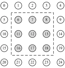
where dimension is the dimension of the group, start rank is the rank of the starting node, and theiteration length stridepair is the iteration and stride of the corresponding dimension. As an example, consider the row-major grid topology in Figure 2.2. The shaded nodes form a communication group. This group is represented as ranklist
<2 6 3 5 3 1>,
where the tuple indicates that this communication group is a 2-dimensional area starting at node 6 with 3 iterations of stride 5 in the y-dimension and 3 iterations of stride 1 in the x-dimension, respectively. Since this encoding scheme takes node placement into account, it naturally reflects the spatial characteristics of a communication group.
Figure 2.2: Ranklist Representation for Communication Group
2.3
Preserving Time in Communication Traces
pro-cesses, “delta” times representing the computation between communication events are recorded and compressed. For the purpose of scalability, delta times of a single MPI function call across multiple loop iterations and across MPI tasks are not recorded one by one. Instead, histograms with a fixed number of bins for delta times are dynamically constructed to provide a statistical view. Delta times are distinguished by not only the call context of recorded events, but also by their path sequence, which addresses significant variation of delta times caused by path differences, e.g., within entry/exit paths of a loop.
2.4
ScalaReplay
Chapter 3
ScalaExtrap: Trace Extrapolation
for SPMD Programs
3.1
Introduction
Scalability is one of the main challenges for scientific applications in HPC. A host of automatic tools have been developed by both academia and industry to assist in communication gathering and analysis for MPI-style message passing [34]. Most of these tools either obtain lossless trace information at the price of poor scalability [52] or preserve only aggregated statistical trace information to limit the size of trace files as in mpiP [75]. Recent work on communication tracing and time recording made a breakthrough in this realm. ScalaTrace introduced an effective communication trace representation and compression algorithm [56]. It managed to preserve the structure and temporal ordering of events, yet maintains traces in a space-efficient representation. However, ScalaTrace needs to be linked to the original application and executed on a high-performance computing cluster of agiven number of compute nodesto obtain a trace. Due to the often long application execution times and limited availability of cluster resources for large numbers of nodes, obtaining the trace information of a large-scale parallel application remains costly.
scale without necessitating time-consuming execution. Specifically, we extrapolate two aspects of the application behavior, namely (1) the communication trace events with parameters and (2) the timing information resembling computation. The extrapolation of the communication trace is based on the observation that, in many regular SPMD stencil and mesh codes, com-munication parameters and comcom-munication groups are related to the sizes and dimensions of the communication topology. Thus, extrapolation of communication traces becomes feasible with the detection of communication topologies and the analysis of communication parameters to infer evolving patterns. The extrapolation of timing information involves a process of ana-lytical modeling. In order to mitigate timing fluctuations under scaling, we employ statistical methods.
Our extrapolation methodology is applicable for both strong and weak scaling applications. Weak scaling is typically defined as scaling the problem size and the number of processors at the same rate such that the problem size per processor is fixed. This should imply that the communication patterns generally evolve in a similar manner for both strong and weak scaling. Thus, we hypothesize that the same extrapolation algorithms for patterns and communication end points should apply to both. For communication parameters, such as message sizes and computation times different trends can be observed. But we hypothesize that extrapolation based on curve fitting is still applicable. In this work, we verify these hypotheses by evaluating our extrapolation algorithm with both strong and weak scaling applications.
Our extrapolation approach follows a trace analysis methodology independent of the tracing infrastructure and works for any of the existing trace formats. Nonetheless, the approach is significantly facilitated by ScalaTrace’s compression scheme that preserves application struc-ture with inherent compression that closely resembles the loop strucstruc-ture of an application. In contrast, extrapolation with other trace formats, such as OTF [40], would be far more tedious and time/space consuming as structure is neither established across nodes nor retained after binary-level compression.
extrapo-lation of timing information resembles the running time of the original parallel application. Compared to the running time of the original application, the accuracy of replay times of the corresponding extrapolated trace is, in the majority of cases, higher than 90%, sometimes as high as 98%. Given the difficulty of extrapolating application execution time with only the time information obtained from several small executions, our approach achieves unprecedented accuracy that is sufficient for modeling, procurement and analysis tasks.
Overall, this work explores the potential to extrapolate communication behavior of par-allel applications. Several novel algorithms for communication topology detection and com-munication trace extrapolation are introduced. Experimental results demonstrate that rapid generation of an application’s trace information at arbitrary size is entirely possible, which is unprecedented. In contrast to tedious and application-centric model development, our ap-proach opens new opportunities for automatically deriving communication models, facilitating communication analysis and tuning at any scale. Our work further enables system simula-tion at extreme scale based on a single file, concise communicasimula-tion trace representasimula-tion. More specifically, HPC simulation tools (e.g., Dimemas or SST [44, 73, 65]), which currently cannot operate at petascale levels, could benefit by utilizing our extrapolated single-file traces that are just 10s of megabytes in size. Benchmark generation is important for cross-platform per-formance analysis due to its standard and portable source code and the platform-independent nature. Our work enables code generation at extreme scale by providing large traces that are otherwise unavailable. Furthermore, by contributing a set of detection techniques of communi-cation patterns, our work has the potential to enable the generation of flexible and stand-alone programs that can be executed with arbitrary numbers of nodes and any possible input.
3.2
Communication Extrapolation
This work focuses on the extrapolation of communication traces and execution times. The respective design is subsequently implemented in a novel tool, ScalaExtrap. The challenge of communication trace extrapolation is to determine how the communication parameters change with node and problem scaling. The main idea is to identify the relationship between commu-nication parameters and the characteristics of the commucommu-nication topology, i.e., typically the sizes of each dimension. As a simple example, in Figure 2.2, assumenode 0 communicates with node 4, i.e., a node at distance of 4. If we can identify that the topological communication space is a grid consisting of 25 nodes with 5 nodes per row, we know that node 0 actually communicates with the upper-right node. Therefore, when there are 1024 = 32×32 nodes, we can safely infer that node 0communicates withnode 31, which is still the upper-right node.
communication pattern from the communication graph provided by a trace file is equivalent to solving the graph isomorphism problem, which is known to be NP hard [87]. Therefore, instead of attempting to find a universal solution, we constrain our work to applications where
1. nodes execute the same program on different data, i.e., the application follow the SPMD paradigm;
2. nodes are numbered in a row-major fashion; and
3. communication is performed in stencil/mesh point-to-point manner or via collectives in-volving all MPI tasks.
In essence, our communication trace extrapolation algorithm first identifies the nodes at the “corner” of a topological space. It then calculates the sizes of each dimension of the topological space accordingly.
Upon acquiring the topology data, we can perform extrapolation. The extrapolation of a communication trace consists of two tasks. First, we need to match the records corresponding to the same MPI call in the source code across the traces of different node sizes. We will discuss the difficulties involved in this step and our solutions in the following sections. Second, for each MPI call in the source code, we need to determine which MPI processes execute this call and what are the values of the parameters when the application is running at the target scale. For the second task, we represent the ranklist and the communication parameters, e.g., the destination rank of MPI Send, as a function of the known topology data and their undetermined coefficients. In order to calculate these coefficients, we correlate multiple traces and construct a set of linear equations. Finally, we employ Gaussian Elimination to solve the set of equations. With the fixed coefficients, we can extrapolate the value of the desired communication parameter by simply substituting the topology data with their values at the desired problem size.
The second aspect of this work concerns the extrapolation of program execution time. In the input trace files, computation time and communication time between (and optionally dur-ing) MPI communication events are preserved statistically with histograms. When analyzing the corresponding delta time, scaling trends can be identified across different number of nodes. Therefore, statistical curve fitting methods are utilized to model an evolving trend and extrap-olate the execution time to a desired target size. In order to eliminate outliers, we further introduce several confidence coefficients to statistically determine the best extrapolated value under such constraints.
3.2.1 Topology Identification
topo-logical space, which we call critical nodes. We devised a three-step approach to identify the communication topology.
1. We create an adjacency list of communication endpoints for each node and group nodes according to their adjacency lists.
2. We identify critical nodes by analyzing the adjacency lists.
3. We calculate the sizes of each dimension (x, y, and z) of the communication topology.
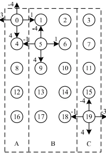
Figure 3.1: Topology Detection Figure 3.2: Boundary Size Calculation
First, our algorithm traverses the input trace to construct communication adjacency lists for each node. According to the relative positions (encodings) of all the communication endpoints of each node, nodes with same endpoint patterns are placed into the same group. Figure 3.1 illustrates an example of a 2D mesh topology. In this example, nodes on the boundaries communicate with nodes at the opposite side in a wrap-around manner while the internal nodes communicate with their immediate neighbors. Note that wrapping around in the vertical direction does not lead to different endpoint encoding. Therefore, the nodes are divided in to three groups (A, B, and C) with group sizes 5, 10, and 5, respectively.
i.e.,critical groups, are calculated as
critical group size= n
length of loop,
wherendenotes the number of nodes engaged in MPI communication. For example, in Figure 3.1, each row has the same group distribution (A B B C) and is thus identified as a single iteration of the loop structure. Since the length of such a loop iteration is 4, the size of the critical groups (group A and C) is 20/4 = 5. Having obtained the size of the critical groups, we then associate critical nodes with groups by matching sizes of critical groups.
Finally, we calculate the sizes of each dimension. Again exploiting the row-major constraint, in a d-dimensional topological space, the number of nodes at the d-th dimension is the total number of nodes. The number of nodes at thei-th (i < d)dimension, ni, is the inclusive range
of numbers of nodes betweennode 0(1stcritical node) and the 2i-thcritical node. Once we have
determined the number of nodes at each dimension, the boundary size of the i-th dimension,
si, is calculated as
si= ni ni−1
For example, in the 3D topology of Figure 3.2, the number of nodes in the 1st dimension,
n1=3, is the number of nodes between A and B inclusively, the number of nodes in the second
dimension, n2=12 , is the number of nodes between A and D, and the number of nodes in the
third dimensionn3 is the total number of nodes. Hence, we have
x=s1=n1/n0= 3 y=s2 =n2/n1 = 4 z=s3=n3/n2
3.2.2 Matching MPI Events for Extrapolation
The extrapolation of a trace is performed one-by-one for each recorded MPI event of the trace. An MPI event is emitted per execution of an MPI function in the source code by the actual values of the input parameters. Therefore, the extrapolation of an MPI event is actually the process of inferring the execution of an MPI function at the target scale from its executions at smaller scales, which are represented as RSDs in the input traces. (In addition, due to the SPMD nature of parallel applications, the extrapolation also involves the prediction of the participants of an MPI event, i.e., the callers of an MPI function in the source code, which will be discussed in Section 3.2.3.) Therefore, being able to match the RSDs corresponding to calls to the same MPI function originating from source code across traces of different node sizes is the prerequisite of extrapolation.
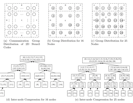
(a) Communication Group Distribution of 2D Stencil Codes
(b) Group Distribution for 16 Nodes
(c) Group Distribution for 25 Nodes
(d) Inter-node Compression for 16 nodes (e) Inter-node Compression for 25 nodes
Figure 3.3: Inter-node Compression and the Positions of Communication Groups
the 25-node trace (in the root node of Figure 3.3(e)) . This illustrates how the order of different communication groups are determined along with the radix tree style inter-node reduction (cf. Figures 3.3(d)+(e)). Clearly, extrapolating by relating RSDs of different communication groups is meaningless.
Algorithm 1 Aligning the Communication Groups Precondition: Tin: input trace
Postcondition: Tout: output trace in which branches (RSD subsequences for communication
groups) are ordered by rank
1: procedure reorder trace(Tin) 2: for iter← Tin.head,Tin.tail do
3: if iter is a merging RSD nodethen
4: merging node ← iter
5: find branching node: merging node’s matching branching RSD node
6: reorder(merging node,branching node) ⊲ reorder the branches between
merging nodeand branching node by rank
7: end if
8: end for
9: end procedure
10: procedure reorder(merging node,branching node)
11: for each branch betweenmerging nodeand branching node do
12: traversebranch in depth-first order
13: if m: a merging RSD node is found in branchthen
14: find b: m’s matching branching RSD node
15: reorder(m,b) ⊲recursively reorder the branches
16: end if
17: end for
18: sort the branches betweenmerging node and branching node by rank
19: reorder the branches
20: end procedure
always organized in ascending order of the rank for the leading nodes of groups. With such an algorithm, we are able to align the communication groups in traces of different node sizes. The extrapolation is subsequently becomes possible.
3.2.3 Extrapolation of MPI Events
The extrapolation of an MPI event consists of the extrapolation of both communication groups and communication parameters to indicate who communicates and how they communicate. The extrapolation algorithm is based on the observation that, in regular SPMD stencil/mesh codes, strong scaling (increasing the number of nodes under a constant input size) linearly increases/decreases the value of communication parameters and the topological sizes. Given several data points, a fitting curve can be constructed to extrapolate the growth rate of the communication parameters and the topology information (the sizes of each dimension) of the communication groups.
Specifically, in an n-dimensional Cartesian space, the coordinates of node X and Y are (X1, X2, ..., Xn) and (Y1, Y2, ..., Yn), where Xi and Yi ∈[0, Si−1] andSi is the size of the i-th
dimension of the topological space (1≤i≤n). Assuming the locations of nodeX andY differ only in thei-thdimension, the distance betweenX andY in the i-thdimension isdi =Xi−Yi.
With the assumption of linear correlation between topology size and communication parameters,
di=Xi−Yi =ai×Si+bi, whereai andbi are two constants. Furthermore, with the row-major
node placement assumption, the rank of an arbitrary node A(A1, A2, ..., An) is
RankA=
n X
i=1 Ai
i−1 Y
j=1 Sj.
Therefore, di′, the rank distance betweenX andY, is
di′ = (Xi−Yi)× i−1 Y
j=1
Sj = (ai×Si+bi)× i−1 Y
j=1 Sj
their rank distances in each dimension,
d′ =d0′+d1′+...+dn′
=
n X
i=1
(Ni−Mi) i−1 Y
j=1 Sj =
n X
i=1
(ai×Si+bi) i−1 Y
j=1 Sj
=an n Y
j=1 Sj +
n−1 X
i=1
(ai+bi+1) i Y
j=1
Sj+b1= n X i=0 ci i Y j=1 Sj,
wherecn=an,c0 =b1, and ci=ai+bi+1(1≤i≤n−1).
In order to extrapolate the rank of a communication endpoint (src/dest), which is defined by the rank distance between nodes, we need to identify how the topology information is related to the communication parameter. We construct a set of linear equations to solveci (1≤i≤n-1). In
general, for an n-dimensional topology,n+ 1 input traces are needed to solven+ 1 coefficients. We employ Gaussian Elimination to solve the equations. Once the values of ci(1≤i≤n−1)
are determined, a fitting curve for the given parameter is established. In order to extrapolate the same parameter for a larger execution, we utilize the known coefficients and specify the topology information at the target task size. The desired value is then calculated accordingly.
As an example, in a 2D space, the bottom-right node in Figure 3.4 communicates with its EASTneighbor in a wrap-around manner. In order to extrapolate the rank of the communica-tion endpoint, three input traces with dimensions 4×4, 5×5, and 6×6 are used to construct the set of linear equations shown in Figure 3.5, andc2 = 1,c1 =−1, andc0 = 1 are obtained as
the values of the coefficients. To extrapolate a 10×10 mesh, we re-construct the equation with coefficients and topology information assigned. Subsequently, the target valueV is calculated asV =c2×10×10 +c1×10 +c0= 91.
Figure 3.4: Generic Representation of Communication Endpoints
c2×4×4 +c1×4 +c0 = 13 c2×5×5 +c1×5 +c0 = 21 c2×6×6 +c1×6 +c0 = 31
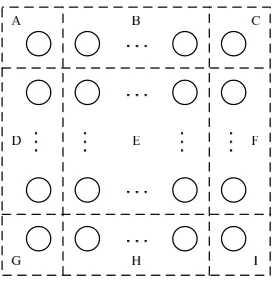
Besides the communication parameters, communication groups are also extrapolated. The topological space of an application can be partitioned into several communication groups ac-cording to the communication endpoint pattern of each node. Under strong scaling, partitions tend to retain their position within the topological space but change their sizes for each dimen-sion accordingly. For example, Figure 3.6 shows the distribution of 9 communication groups of a 2D stencil code. Despite the changing problem size, groups A,C,G, andI always represent corner nodes, groups B, D, F, and H are always the boundaries, and group E contains the remaining (interior) nodes.
Figure 3.6: Distribution of Communication Groups of a 2D Stencil Code
This opens up the opportunity to extrapolate communication groups of the same application at arbitrary size. In order to extrapolate, we represent communication groups as ranklists, which effectively specifies the starting node and the dimension sizes of a group. Since the dimension sizes are defined by the distances between nodes (vertices), we again utilize a set of linear equations to establish the relation between the topology information of communication groups and the task sizes. Extrapolation is performed for thestart rank,iteration length, andstride fields of the ranklist. The output ranklist reflects the communication group at the target size. For example, for the topology shown in Figure 3.6, when the total number of nodes is 16, the ranklist of groupE, as defined in Section 2.2, is <2 5 2 4 2 1>, i.e., a 2D space starting from node 5 with x- and y-dimensions of size 2. Similarly, the ranklists of group E at sizes 25 and 36 are <2 6 3 5 3 1>and <2 7 4 6 4 1>, respectively. We can thus construct the set of linear equations for each field in the ranklist to derive a generic representation of the ranklist as:
Subsequently, assuming that we want to extrapolate for size 10× 10, let x be 10, which yields the output ranklist<2 11 8 10 8 1> that precisely matches the ranklist representation of communication groupE at this problem size.
By combining the extrapolation of both communication groups and communication pa-rameters, we are capable of extrapolating the communication trace for a given application at arbitrary topological sizes.
3.2.4 Lossy Extrapolation
As was discussed in Section 3.2.2, aligning the matching RSDs across traces of different node sizes is critical for extrapolation. Despite being recognized as one of the existing tracing li-braries that provides the best compression, there still exist some applications that ScalaTrace cannot obtain constant-size compression for. In fact, for applications that exhibit new commu-nication patterns only at or beyond a certain node size, lossless yet constant-size compression is hardly possible. To extrapolate traces of such applications, we designed a lossy but still pro-gram structure-preserving approach. We attempt to capture and extrapolate the dominating communication pattern by optionally dropping events at three different levels: (1) within an MPI process, (2) among MPI processes of an execution, and (3) across traces of different node sizes.
The intra-node level event filtering is performed against the per-node queue of MPI events. We observe that a number of application traces contain a subsequence of events that embody the dominating communication pattern and comprise a large portion of the trace by repeating multiple times. Based on this observation, a user-provided trace snippet is utilized as the reference to drop events. Typically, such a trace snippet is a sequence of RSDs consisting of tens of MPI events, with the event type (Send, Recv, etc.) and the values of the key parameters of each event. Based on the trace snippet, we automatically generate a Finite-State Machine (FSM) to process the input stream of MPI events. At the beginning, the FSM is initialized to the START state. If the input event is a collective, the FSM directly enters the ACCEPT state. This indicates that all collectives are directly accepted while the FSM is not in the middle of accepting a sequence. If the input is neither a collective nor the first event to be accepted, the FSM enters the ERROR state and the input event is dropped. Once the FSM leaves the START state, it only accepts the next event expected in a sequence. If an unexpected event arrives, the FSM enters the ERROR state and all the pending events are dropped, including the current input if it is not a collective. Finally, if the FSM arrives at the ACCEPT state, the pending events are accepted. These events will not be affected by future ERROR states. Figure 3.7 shows a simple trace snippet and the FSM generated.
inter-<MPI_Irecv, (LEFT)> <MPI_Isend, (RIGHT)> <MPI_Wait>
<MPI_Wait>
(a) Trace Snippet (b) Generated Finite-state Machine
Figure 3.7: A Simple Trace Snippet and the Generated Finite-state Machine
node compression and when aligning the traces of different node sizes for extrapolation. We designed a Longest Common Subsequence (LCS) based approach for the event filtering at these two levels. The LCS problem is to find the longest subsequence that is common to two input sequences, where a subsequence need not be consecutive in either of the original sequences. If a trace is considered as a sequence of MPI events, the LCS of two traces reflects the MPI events that nodes participate in for both traces. We adapted a well-known dynamic programming based LCS algorithm for trace comparison [9]. In a ScalaTrace trace, the loop structure is preserved and explicitly indicated. As a building block, loop structures should be evaluated in their entirety with the number of MPI events in the loop representing the weight. Therefore, we first enhanced the LCS algorithm to take into account the weight when evaluating how the length of the LCS will be affected by retaining or removing a loop structure. Second, since loops are often nested in the source code and in the trace, we further modified the LCS algorithm so that it can execute in two modes in a recursive manner. In the first pass, this algorithm only calculates the LCS but does not modify the trace. This is required because modifying the inner loop may affect the evaluation of the outer loop. Once the LCS is determined, this algorithm is applied again in the second mode such that any uncommon events are removed.
3.2.5 Extrapolation of Timing Information
Besides the communication traces, we also extrapolate the timing information of the application. ScalaTrace preserves the “delta” time for each communication event and for the computation between two communication events. For a single MPI function call across multiple loop itera-tions, i.e., for a RSD, the delta times are recorded in multi-bin histograms. These histograms contain the overall average, minimum, and maximum delta time, the distribution of the delta execution times represented as histogram bins, and the average, minimum, and maximum delta time for each histogram bin. To extrapolate timing information, we utilize curve fitting to capture the variations in trends of the delta times with respect to the number of nodes, i.e.,
t= f(n), where tis the delta execution time and n is the total number of nodes. Hence, the target delta time te is calculated as te = f(ne), where ne is the total number of nodes at a
given problem size. While we can extrapolate only the aggregated average delta time per RSD, to restrain the statistics of delta time, extrapolation is performed for each field of a histogram. Currently, we implemented four statistical models based on curve fitting for each extrapolation. We use a deviation-based metric to determine the best of these models to fit to a given curve.
1. Constant: This method captures constant time, i.e.,t=f(n) =c. Before calculating the constant time, the input time to with the largest absolute value of deviation is excluded
from the input times to mitigate the influence of outliers (which can be caused by either unstable system state or an empty bin). Subsequently, the average value of the remaining input times reflects the constant timec, and d1 =std. dev./average is used to evaluate
this fitting curve among the remaining values.
2. Linear: This method captures linearly increasing/decreasing trends, i.e.,t=f(n) =an+
b. We use the least-squares method to fit the curve. In order to avoid mis-classifications, such as a constant time relationship as a linear relationship with a near-zero slope, we define a threshold slope smin = 0.2 such that ∀a < smin, t = f(n) = b. For curve
evaluation, d2 = √
residual/average is used, where average refers to the average value of the estimated running times.
3. Inverse Proportional: This method captures inverse-proportional trends, i.e., t=f(n) =
k/n. We observe this trend in the NAS Parallel Benchmark IS, where MPI Alltoallv dynamically rebalances the per-node workloads even though the collective workload over all nodes is constant. Lettibe the input times,ni be the corresponding number of nodes,
and ki = ti×ni. We extrapolate the constant k as the average value of ki. Again, we
exclude the outlier ko, which has the largest absolute value within the deviation. To
evaluate this fitting curve, we calculate the standard deviation of ki and then divide by
4. Inverse Proportional + Constant: This method captures the execution time consisting of an inverse proportional phase and a constant phase, i.e., t=f(n) = k/n+c. Instead of directly extrapolatingt, we utilize the least-squares method to extrapolatet′=tn=cn+k
and use d4 = √
residual/average for the curve evaluation. With an extrapolated c and
k,tis subsequently calculated as t=t′/n=k/n+c.
Having obtained the deviations for each curve-fitting process, we compare the values to determine the curve that best fits. For a closer approximation, we define a threshold value
dt = 0.05, such that if and only if dmin +dt < di holds for all di other than dmin will the
corresponding candidate curve be selected as the fitting curve. Otherwise, the extrapolation for the current field is postponed until we have processed all the fields in the same histogram. Since every field in the histogram should have the same variation trend, we finalize the pending extrapolation according to the decisions of the remaining fields.
3.3
Experimental Framework
Our extrapolation methodology for communication traces was implemented as the ScalaExtrap tool that generates a synthetic trace for a freely selected number of nodes. The extrapolation is based on traces obtained from application instrumentation with ScalaTrace on a cluster. For both base traces generation and results verification, we use a subset of JUGENE, an IBM Blue Gene/P with 73,728 compute nodes and 294,912 cores, 2 GB memory per node, and the 3D torus and global tree interconnection networks.
The extrapolation process is run on a single workstation and requires only several seconds, irrespective of the target number of nodes for extrapolation. This low overhead is due to the linear time complexity of our algorithm with respect to the total number of MPI function calls in an application. Results from extrapolation are subsequently compared to traces and runtimes of an application at the same scale, where runtimes for extrapolated traces are obtained via ScalaReplay (see Section 2.4).
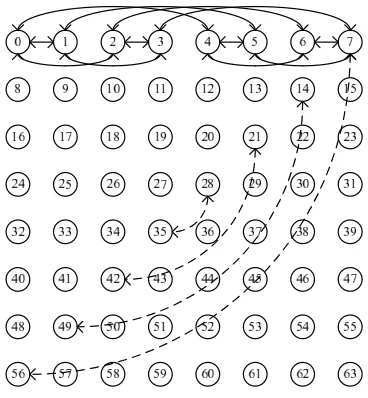
communicates with the nodes in the same row with a power-of-two distance and with the node diagonally symmetric to itself, as indicated in Figure 3.8. We support such more complicated patterns by allowing programmers to provide plugin functions for compression and extrapola-tion on a per-parameter basis. The communicaextrapola-tion trace extrapolaextrapola-tion for CG is facilitated by specifying the communication pattern (i.e., the communication end point described by a func-tion) as a plugin. With this plugin, the extrapolation of timing information does not require any extra information.
Figure 3.8: CG Communication Topology
We report the experimental results for both strong scaling and weak scaling. For the strong scaling experiments, we mostly used class D and E input sizes for the NPB codes. For the weak scaling experiments, we enhanced the input generator to provide weak scaling inputs for selected NPB codes.
3.4
Experimental Results
of nodes.
3.4.1 Correctness of Communication Trace Extrapolation
We first evaluated our communication trace extrapolation algorithm with microbenchmarks and the NPB BT, EP, FT, CG, LU, and IS codes. We assessed the ability to retain communi-cation semantics across the extrapolation process for these benchmarks at the target scale. The microbenchmarks perform regular stencil-style/torus-style communication in topological spaces from 1D to 3D. The NPB programs exercise both collective and point-to-point communication patterns. We verified the extrapolation results in multiple ways.
1. The extrapolated trace fileTe0 was compared with the trace file obtained from an actual
execution at the same scaleTtarget on a per-event basis (Exp1 in Figure 3.9).
2. The extrapolated trace Te0 was replayed such that aggregate statistical metrics about
communication events could be compared to those of a corresponding original application run at the same problem size and node size (Exp2 in Figure 3.9).
3. After extrapolation, traces Te1, Te2, ..., Tei were collected in a sequence of replays to
obtain a fixed point in the trace representation (Exp3 in Figure 3.9).
Figure 3.9: Correctness of Trace Extrapolation and Replay
nodes. However, it diverges slightly from an inverse-proportional approximation for extrapo-lating the message volume due to integer division (discarding the remainder) inherent to the source code. This inaccuracy is later amplified in the extrapolation process and results in mes-sage volumes that are about 13% smaller than the actual ones at a given scaling factor in the worst case. As imprecisions remain localized to certain point-to-point messages, this effect is shown to be contained in that resulting timings are deemed accurate within the considered tolerance range for extrapolation experiments (see timing results below). Such imprecisions have no side-effect on semantic correctness (causal order) of trace events whatsoever. Overall, the results of static trace analysis show that our synthetically generated extrapolation trace is equivalent to the trace obtained from actual execution of the same application at the same scaling level.
Second, we replayed the extrapolated trace Te0 to assess if the MPI communication events
are fully captured (see Exp2 in Figure 3.9). For this experiment, ScalaReplay is linked with mpiP [75], which yields frequency information of each MPI call distinguished by call site (us-ing dynamic stackwalks). Dur(us-ing replay, all MPI function calls recorded in the synthetically generated extrapolation trace were executed with the same number of nodes and their orig-inal payload size. For comparison, we instrumented the origorig-inal application with mpiP and executed it at extrapolated sizes (problem and node sizes). We compared the Aggregate Sent Message Sizereported by mpiP between the original application and the replayed extrapolated trace. Results show that the total send volumes of these experiments are identical, except for MPI Isend in BT as discussed above. We also compared the total number of MPI calls recorded in the mpiP output files. The results allowed us to verify that the number of communication events in the actual and extrapolated traces match, i.e., the correctness of communication trace extrapolation is preserved.
Third, we evaluated the correctness of ScalaReplay by replaying the generated trace file in sequence until a fixed point is reached (see Exp3 in Figure 3.9). The fixed point approach is a well established mathematical proof method that establishes conversion, in this case of the trace data. In this experiment, instead of instrumenting ScalaReplay with mpiP, we interposed MPI calls through ScalaTrace again. As ScalaReplay issues MPI function calls, ScalaTrace captures these communication events and generates a trace file for it, just as would be done for any other ordinary MPI application. We start by replaying the extrapolated trace file Te0 and
obtain a new trace Te1. This trace differs from Te0 in that call sites of the original program
have been replaced by call sites from ScalaReplay. This affects not only stackwalk signatures but also the structure of trace files due to the recursive approach of replaying trace files in place over their internal (PRSD) structure without decompressing it. We then replay trace Te1 to
obtain another trace Te2 and so on for Tei. We then compare pairs of trace filesTei, Tei+1. If
pairs of trace files, baring syntactical differences, are semantically equivalent to each other. In other words, ScalaReplay neither adds nor drops any communication events during replay, i.e., by obtaining a fixed point it was shown that all MPI communication calls are preserved during replay.
3.4.2 Accuracy of Extrapolated Timings: Timed Replay
We further analyzed the timing information of the extrapolated traces. We report the accuracy of the extrapolated timings for both strong scaling and weak scaling.
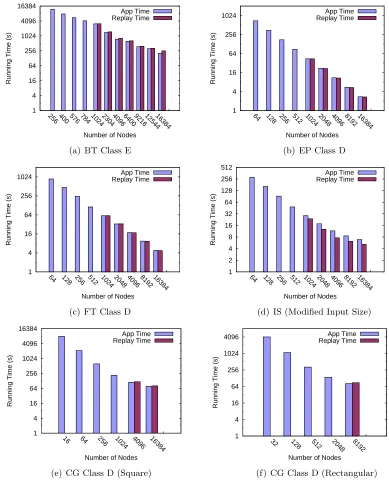
Strong Scaling: For this set experiments, we used the NPB BT, EP, FT, CG, and IS codes with a total number of nodes of up to 16,384. For CG, EP, and FT, we used class D input sizes. For BT, class E was used so that a sufficient workload is guaranteed at 16,384 nodes. For IS, we modified the input size to adapt it for 16,384 nodes (the original NPB3.3-MPI provides only class D problem size and supports a maximum of 1024 nodes). These problem sizes and node sizes were decided based on the memory constraints (for some benchmarks, memory constraints compel us to generate the base traces already at large scales, which in turn leaves fewer target sizes for evaluation) and the availability of computational resources to assess the effects and limitations of our timing extrapolation approach.
In this set of experiments, we first generated 4 trace files for each benchmark as the ex-trapolation basis. From these base traces, an extrapolated trace was constructed next using ScalaExtrap, including extrapolated delta time histograms. We then assess the timing accuracy by replaying the extrapolated traces. During replay, ScalaReplay parses the timing histograms of the computation periods in the trace files. It simulates computation by sleeping to delay the next communication event by the proper amount of time. In this context, the effect of load imbalance is preserved by ScalaTrace. The timing histogram records not only minimum, maximum, average and standard deviation values, but also the frequency for each timing bin, and these statistics are also extrapolated by ScalaExtrap. During replay, the sleeping time is generated according to these statistics and the unbalanced timing behavior is thus reproduced. Communication is simply replayed with the same extrapolated end points and payload sizes but a random message payload. We do not impose any delays on communication as published results indicate better accuracy with just delays for computation only [56], which we also con-firmed. In this experiment, ScalaReplay is linked to neither ScalaTrace nor mpiP to avoid additional overhead caused by the instrumentation layer of these tools. Hence, the output of ScalaReplay in this experiment is the total time to replay a trace. For each extrapolated trace, we run the corresponding application at the same problem size and record its overall execution time for comparison.
1 4 16 64 256 1024 4096 16384
256 400 576 784 102423044096640092161254416384
Running Time (s)
Number of Nodes App Time Replay Time
(a) BT Class E
1 4 16 64 256 1024
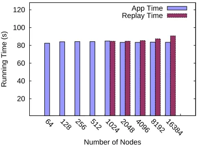
64 128 256 512 1024 2048 4096 8192 16384
Running Time (s)
Number of Nodes App Time Replay Time
(b) EP Class D
1 4 16 64 256 1024
64 128 256 512 1024 2048 4096 8192 16384
Running Time (s)
Number of Nodes App Time Replay Time
(c) FT Class D
1 2 4 8 16 32 64 128 256 512
64 128 256 512 1024 2048 4096 8192 16384
Running Time (s)
Number of Nodes App Time Replay Time
(d) IS (Modified Input Size)
1 4 16 64 256 1024 4096 16384
16 64 256 1024 4096 16384
Running Time (s)
Number of Nodes App Time Replay Time
(e) CG Class D (Square)
1 4 16 64 256 1024 4096
32 128 512 2048 8192
Running Time (s)
Number of Nodes App Time Replay Time
(f) CG Class D (Rectangular)
Figure 3.10: Replay Time Accuracy for Strong Scaling Benchmarks
higher than 98%, where accuracy is defined as
Accuracy = (1−|Replay T ime − App T ime|
App T ime )×100%.
For BT, we observed slightly lower accuracy when the total number of nodes approaches 16,384. At such sizes the computational workload becomes so small that the influence of non-deterministic factors, such as system overheads or performance fluctuation of MPI collectives caused by different process arrival patterns [27], become dominant. Compared to the other benchmarks, IS shows a constantly lower accuracy (66%-83%). Two reasons may explain this phenomenon: (a) Although IS dynamically rebalances the workload across all nodes, the exe-cution time of the application’s sorting algorithm on each process still takes a different amount of time. Hence, collective MPI calls take unpredictable time to synchronize as the arrival times of processes at collectives varies significantly due to load imbalance. Since the degree of im-balance is determined by randomly determined delta times from histograms, it is difficult to predict/extrapolate this behavior. (b) Source code analysis shows that the most computation-ally intensive code section in IS consists of two phases, namely (i) an inverse-proportional phase (runtime is inverse-proportional to the number of nodes), and (ii) a relatively short constant phase (runtime does not change significantly with node sizes). When the node size is small, the inverse-proportional phase almost solely determines the computation time. As a result, our algorithm fails to uncover a small constant factor that contributes to timing for larger node sizes. ScalaExtrap instead treats it as a pure inverse-proportional timing trend. Without the short constant factor in the timing curve, the extrapolated runtime drops slightly faster than the real runtime leading to a constantly shorter replay time. However, since we are able to cap-ture the dominating inverse-proportional timing trend, we still obtained an acceptable timing prediction accuracy.
In large, minor inaccuracies during replay stem from imprecise curve fitting for the ex-trapolation of computation times. For the simulation of communication duration, ScalaReplay depends only on the communication parameters such as end points and payload sizes, which are shown to be correctly extrapolated in Section 3.4.1. Overall, the extrapolated timing infor-mation precisely reflects the runtime of the original application at the target problem size and node size.
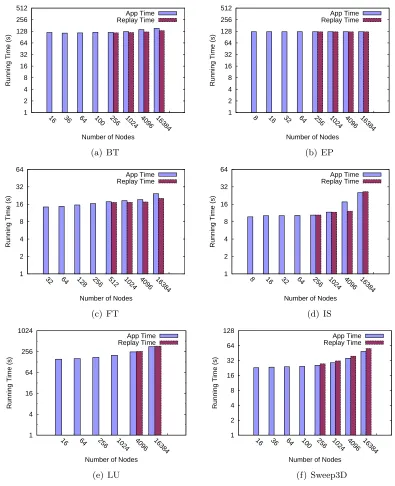
ex-trapolation algorithms still apply to weak scaling codes. For the other two factors, compared to strong scaling codes, weak scaling codes may exhibit different runtime behavior. For example, due to a constant computational workload per node, the computation times often (but not always) follow a constant trend for weak scaling. In terms of the message sizes, the overall message volume exchanged among all the participating nodes—typically with MPI Alltoall or MPI Alltoallv—often increases linearly (or remain constant) under weak scaling when varying the total number of processes. Nonetheless, the curve fitting approach is still applicable, though different/additional curve fitting algorithms may have to be supplied in practice.
We verified our extrapolation approach with weak scaling codes. We conducted these ex-periments with the NPB BT, EP, FT, IS and LU codes, and the Sweep3D neutron-transport kernel [79]. (For other NPB codes, such as CG, weak scaling inputs could be easily be con-structed.) Unlike Sweep3D, the NPB codes are originally designed as strong scaling benchmarks. Hence, we manually changed the input to provide weak scaling workloads.
In the first experiment, we verified the correctness of the generated traces with respect to the extrapolated communication topologies and the values of the communication parameters. We applied similar tests, i.e., static trace comparison and mpiP results comparison, for the synthetically generated traces under weak scaling. The results show that the extrapolated traces are able to correctly preserve the communication semantics, and hence demonstrate the applicability of our topology extrapolation algorithm for applications under weak scaling.