Abstract
TAN, PHAIK-HOON. Statistical Analysis of Long-Range Dependent Processes via a
Stochastic Intensity Approach, with Applications in Networking. (Under the direction of James R. Wilson.)
The objective of this research is to develop a flexible stochastic intensity-function
model for traffic arrivals arising in an Ethernet local area network. To test some
well-known Bellcore datasets for long-range dependence or nonstationarity, a battery of
statistical tests was applied—including a new extension of the classical Priestley-Rao test for
nonstationarity; and the results of this analysis revealed pronounced nonstationarity in all
of the Bellcore datasets. To model such teletraffic arrival processes accurately, a stochastic
intensity function was formulated as a nonlinear extension of the Cox regression model
that incorporates a general time trend together with cyclic effects and packet-size effects.
The proposed intensity-function model has an exponential-polynomial-trigonometric form
that includes a covariate representing the latest packet size. Maximum likelihood estimates
of the unknown continuous parameters of the stochastic intensity function are obtained
numerically, and the degrees of the polynomial time and packet-size components are
determined by a likelihood ratio test. Although this approach yielded excellent fits to
the Bellcore datasets, it also yielded the surprising conclusion that packet size has a
negligible effect on the packet arrival rate. A follow-up analysis of the packet-size process
confirmed this conclusion and shed additional light on the packet-generation mechanism in
Ethernet local area networks. This research also includes the development of procedures
for simulating traffic processes having a stochastic intensity function of the proposed form.
An extensive Monte Carlo performance evaluation demonstrates the effectiveness of the
Biography
Phaik-Hoon Tan was born on January 6, 1959 in Alor Star, Malaysia. She graduated with a Bachelor of Engineering in Chemical Engineering from the University of Malaya,
Kuala Lumpur, Malaysia in June 1982. Upon graduation, she worked for the Ministry of Labour, Singapore for a year before returning to Malaysia to join the Malaysian Civil Service
under the National Productivity Center (NPC), later renamed the National Productivity Corporation. In 1989, she was awarded a British Council scholarship for a graduate program
in University of Wales, Cardiff, United Kingdom and graduated with a Master of Science in
Systems Engineering in 1991. Upon her return to Malaysia, she served in the Productivity Research division until 1995 when she was awarded a Federal scholarship to pursue her
Acknowledgments
I thank Prof. James R. Wilson, Chair of my advisory committee, for the knowledge that I have gained from him over the past few years. Also, I thank him for the confidence that
he had instilled in me. I also thank him for the time and effort he put forth for me in the development of this research. I also thank Prof. Arne A. Nilsson for generously extending his
research assistants to help me learn up the area of networking all throughout my research. To Prof. Thom J. Hodgson and Prof. Henry L. Nuttle, I thank them for their serving as
members of my advisory committee as well as for their suggestions. I am greatly indebted
to Dr. Halim Damerdji for his insightful points of view. Although he has not been around to see to the completion of my dissertation, his initial efforts to push me along and his
encouragement has helped me achieve my goals.
This dissertation would not have been without the support of my husband Khai Nam, who
has always been appreciative of my goals and dreams. In particular, I would like to thank him for his sacrifice and dedication in enabling me to get my Ph.D. degree. To my mom
who has been a great source of help during this time, I extend my warmest hugs and love. Lastly, I wish to dedicate this research to both my children, Adeline and Catherine, and
Table of Contents
List of Tables vii
List of Figures ix
1 Introduction 1
1.1 Preliminaries . . . 1
1.2 Problem Formulation . . . 3
1.3 Objectives of the Research . . . 5
1.4 Organization of the Dissertation . . . 6
2 A Brief Overview of Computer Networks 7 2.1 Preliminaries . . . 7
2.2 The Advent of Computer Networks: LANs and WANs . . . 8
2.3 Ethernet . . . 10
2.3.1 The Origin of Ethernet . . . 10
2.3.2 Ethernet Features . . . 10
2.4 ATM . . . 11
2.5 ISDN and Broadband ISDN . . . 12
2.6 Protocols . . . 13
2.6.1 OSI Reference Model . . . 13
2.6.2 Application Protocols . . . 15
2.6.3 Transmission Control Protocol (TCP/IP) . . . 16
3 Traffic Models and Statistical Analysis of Traffic Data : A Literature Review 17 3.1 Preliminaries . . . 17
3.1.1 Self-Similarity . . . 17
3.1.2 Long-Range Dependence (LRD) and Slowly Decaying Variance . . . 18
3.1.3 Heavy-Tailed Distributions . . . 20
3.2 Early Traffic Models . . . 20
3.3 Recent Developments in Traffic Measurements . . . 22
3.4 Self-Similar Traffic Models . . . 24
3.4.1 Fractional Brownian Motion and Fractional Gaussian Noise . . . 26
3.4.2 Autoregressive Traffic Models . . . 27
3.4.2.1 Fractional ARIMA . . . 27
3.4.2.2 Discrete Autoregressive Processes . . . 28
3.4.2.3 TES Models . . . 29
3.5 Simulation of Self-Similar Processes . . . 31
3.6 Statistical Inference for Long-Range Dependent Processes . . . 33
3.7 Statistical Tests for LRD . . . 35
3.7.1 Variance-Time Analysis . . . 36
3.7.2 R/S Analysis . . . 37
3.7.3 Periodogram-Based Analysis . . . 37
3.8 Actual Packet Level Statistics . . . 38
3.9 Summary . . . 39
4 Testing for Nonstationarity 42 4.1 Nonstationarity of Traffic . . . 42
4.2 Description of Teletraffic Datasets Tested . . . 43
4.3 Preliminary Visual Evidence . . . 43
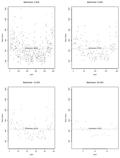
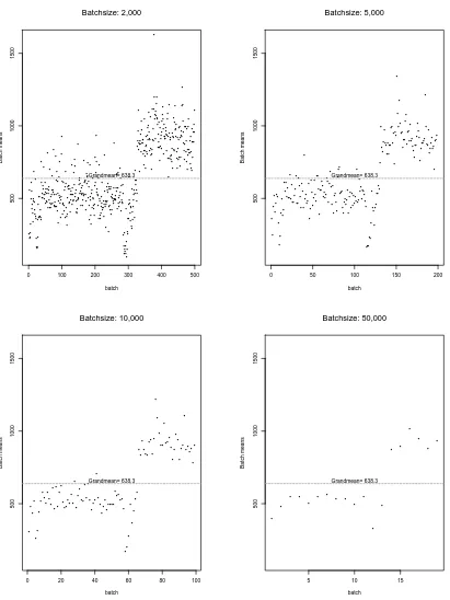
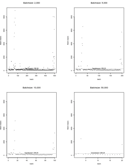
4.3.1 Batch-Means Analysis . . . 44
4.3.2 The von Neumann Test . . . 57
4.3.3 The Dickey-Fuller Test for Nonstationarity . . . 58
4.4 Tests for Covariance Stationarity . . . 59
4.4.1 Postsample Prediction Test for Covariance Stationarity . . . 61
4.4.2 CUSUM Test for Covariance Stationarity . . . 62
4.4.3 Modified Scaled Range Test for Covariance Stationarity . . . 64
4.5 An Extension of the Stationarity Test of Priestley and Rao . . . 66
4.5.1 Basis of the Extended Test . . . 67
4.5.2 Extended Priestley-Rao Test Procedure . . . 70
4.5.3 Results of the Extended Priestley-Rao’s Test . . . 72
4.6 Summary . . . 72
5 A Stochastic Intensity Approach to Modeling Traffic 74 5.1 Point Process Theory . . . 74
5.1.1 Traffic Modeling Using Point Process Theory . . . 76
5.2 Model Formulation . . . 78
5.3 Basic Nomenclature . . . 78
5.4 Parameter Estimation Based on Maximum Likelihood . . . 79
5.4.1 Methods for Estimating Model Parameters . . . 80
5.4.2 Computing Initial Estimates for Trigonometric Parameters . . . 81
5.4.3 Computing Initial Values for Polynomial Coefficients of Time and Packet Size . . . 83
5.5 Computing Final Parameter Estimates . . . 87
5.6 Summary . . . 88
6 Applications to Modeling and Simulation of Teletraffic 90 6.1 An Application to Networking . . . 90
6.2 Presentation of Results . . . 97
6.3 Autoregressive Models of Packet-Size Processes . . . 104
6.3.1 Tests for Stationarity of Packet-Size Processes . . . 104
6.3.3 Estimation of Autoregressive Models for Packet-Size Processes . . . 112
6.4 Summary . . . 112
7 Simulation of Teletraffic Traces 114 7.1 The Simulation Program . . . 114
7.2 Experimental Runs . . . 115
7.3 Performance Evaluation of the Estimation Procedure . . . 116
7.4 Summary . . . 119
8 Conclusions and Further Research 129 8.1 Conclusions . . . 129
8.2 Recommendations for Future Work . . . 130
References 132 Appendices 142 Appendix A. Listing of S-plus programs . . . 142
Appendix B. Listing of S-plus program for Postsample Prediction Test . . . 145
List of Tables
2.1 Layers of the OSI Architecture . . . 14
3.1 Ethernet Traffic Measurements on NCSU Dataset A . . . 39
4.1 Qualitative Description of Files Comprising Dataset B Ethernet Traffic Measurements . . . 44
4.2 Estimated Lag-1 Autocorrelation ˆρ1(`) for Batch Means with Various Batch Sizes . . . 45
4.3 Estimated Autocovariance at Lag Zero, ˆγ(0), for Three Different Sections of the Time Series . . . 50
4.4 Batch Sizes at Which H0 is Rejected (β = 0.10) Applying von Neumann’s Test to the Bellcore Dataset pAug.TL (z0.9 = 1.282) . . . 57
4.5 Dickey-Fuller Tests Applied to Bellcore Datasets for n= 25 . . . 59
4.6 Postsample Prediction Test (4.16) for Bellcore Datasets Based on α= 0.10 . 63 4.7 Modified Scaled Range Test Statistics for Bellcore Datasets . . . 64
4.8 Two-Way Analysis of Variance Spectral Estimates . . . 70
4.9 Analysis of Variance Table for the Bellcore Datasets . . . 73
6.1 Periodogram Analysis of Dataset B Ethernet Traffic Measurements . . . 92
6.2 Parameter Estimates for Dataset B Ethernet Traffic Measurements . . . 98
6.3 Dickey-Fuller Test Applied to Packet Size of Bellcore Datasets . . . 104
6.4 Extended Priestley-Rao Test for Nonstationarity of the Packet-Size Process in the Bellcore Datasets . . . 110
6.5 Autocorrelation at Lag-1 for Dataset B Ethernet Traffic Measurements . . . 111
6.6 Parameters of Fitted AR Process for Dataset B Ethernet Traffic Measurements113 7.1 Parameters for Simulation of Measurements . . . 117
7.2 Estimated Parameters for the Simulated Measurements for 1 replication . . 118
List of Figures
2.1 The Layers of the OSI Reference Model . . . 15
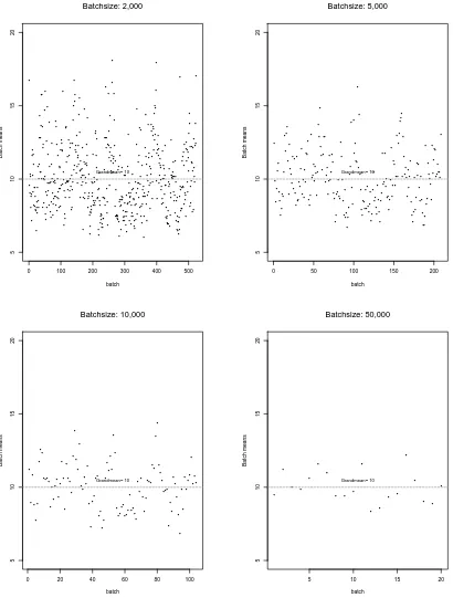
3.1 Variance-Time Plot, R/S Diagram, and Periodogram Plot for DATA1-0814 41 4.1 Plots of Batch Means vs. Batch Sizes for Dataset pAug.TL . . . 46
4.2 Plots of Batch Means vs. Batch Sizes for Dataset pOct.TL . . . 47
4.3 Plots of Batch Means vs. Batch Sizes for Dataset OctExt.TL . . . 48
4.4 Plots of Batch Means vs. Batch Sizes for Dataset OctExt4.TL . . . 49
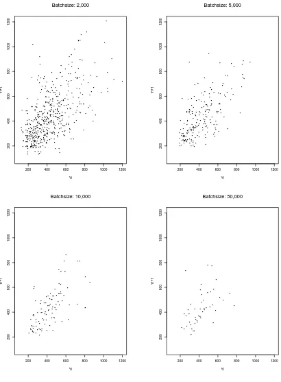
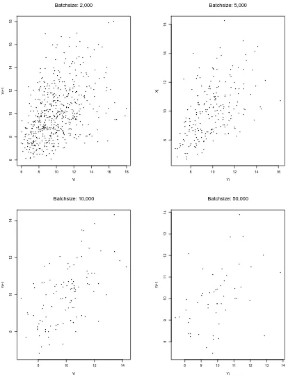
4.5 Scatterplots of Y2j(`) vs. Y2j−1(`) for Various Batch Sizes ` in Dataset pAug.TL . . . 51
4.6 Plots of Batch Means vs. Batch Sizes for Simulated FGN Data withH = 0.90 52 4.7 Scatterplots of Y2j(`) vs. Y2j−1(`) for Various Batch Sizes ` in Simulated FGN Data with H= 0.90 . . . 53
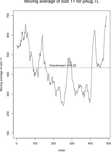
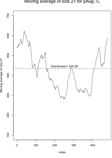
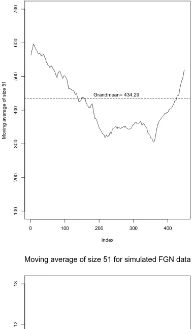
4.8 Moving Average for Bellcore Data and Simulated FGN Data . . . 54
4.9 Moving Average for Bellcore Data and Simulated FGN Data . . . 55
4.10 Moving Average for Bellcore Data and Simulated FGN Data . . . 56
4.11 Recursive Variance Plots of ˆµ2,t vs.tas in (4.9) for the Bellcore Datasets . 60 4.12 CUSUM Plots for the Bellcore Datasets . . . 65
5.1 A Realization of a Point Process and Its Associated Counting Function . . 77
6.1 Histogram Plots for Various Bellcore Datasets . . . 91
6.2 Plot of Estimated Spectrum for Dataset pAug.TL . . . 93
6.3 Plot of Estimated Spectrum for Dataset pOct.TL . . . 94
6.4 Plot of Estimated Spectrum for Dataset OctExt.TL . . . 95
6.5 Plot of Estimated Spectrum for Dataset OctExt4.TL . . . 96
6.6 Plot of Cumulative Arrivals N(t) (Solid Line) versus Fitted Mean-Value Function ˜µ(t) (Dotted Line) for Dataset pAug.TL . . . 99
6.7 Plot of Cumulative Arrivals N(t) (Solid Line) versus Fitted Mean-Value Function ˜µ(t) (Dotted Line) for Dataset pOct.TL . . . 100
6.8 Plot of Cumulative Arrivals N(t) (Solid Line) versus Fitted Mean-Value Function ˜µ(t) (Dotted Line) for Dataset OctExt.TL . . . 101
6.12 Estimated Density Plot for Bellcore Dataset pOct.TL . . . 106
6.13 Estimated Density Plot for Bellcore Dataset OctExt.TL . . . 107
6.14 Estimated Density Plot for Bellcore Dataset OctExt4.TL . . . 108
7.1 90% Tolerance Intervals (Dashed Lines) for Mean-Value Functionµ(t) (Solid
Line), t∈[0,12), in Case 1 . . . 121
7.2 90% Tolerance Intervals (Dashed Lines) for Mean-Value Functionµ(t) (Solid
Line), t∈[0,12), in Case 2 . . . 122
7.3 90% Tolerance Intervals (Dashed Lines) for Mean-Value Functionµ(t) (Solid
Line), t∈[0,12), in Case 3 . . . 123
7.4 90% Tolerance Intervals (Dashed Lines) for Mean-Value Functionµ(t) (Solid
Line), t∈[0,12), in Case 4 . . . 124
7.5 90% Tolerance Intervals (Dashed Lines) for Mean-Value Functionµ(t) (Solid
Line), t∈[0,12), in Case 5 . . . 125
7.6 90% Tolerance Intervals (Dashed Lines) for Mean-Value Functionµ(t) (Solid
Line), t∈[0,12), in Case 6 . . . 126
7.7 90% Tolerance Intervals (Dashed Lines) for Mean-Value Functionµ(t) (Solid
Line), t∈[0,12), in Case 7 . . . 127
7.8 90% Tolerance Intervals (Dashed Lines) for Mean-Value Functionµ(t) (Solid
Chapter 1
Introduction
1.1
Preliminaries
The fundamental purpose of a communications system is the exchange of data between parties—for example, the exchange of voice signals between two telephone users. The
exchange of information between any two communicating pieces of equipment such as
computers, printers, telephones, televisions, and so on, for the purpose of cooperative action is generally referred to as telecommunications. Networking arose from the need to share
data in a timely fashion. For instance, the telephone network can be considered to be the world’s largest telecommunications network because it carries voice, video, facsimile,
and data. It currently supports not only wired telephones, but also fax machines, cellular phones, answering machines, and modems. The Internet is the other major networking
technology. It connects tens of millions of computers around the world, allowing them to
exchange messages and share resources. Internet users can exchange electronic mail, read and post to electronic bulletin boards, access files anywhere in the network, and make
information available to other users.
In this modern age, network systems are being designed to accommodate a heterogeneous
mix of traffic classes ranging from traditional telephone calls to video to data-handling
services. When a piece of information is transmitted over a network, it is divided into packets or cells. Queues may build or partial information may be lost, thus impacting
the quality of the application. To quantify this degradation in quality, a multidimensional performance objective function called Quality of Service (QoS) is defined for each traffic
class (see Schwartz (1996), p. 3). This measure includes such parameters as delay (mean
time jitter (distortion or instability in a signal waveform over time) and throughput.
Both video and voice (audio), being real-time traffic, cannot incur too much jitter during
their journey from source to destination. That is why they require strict timing in their transmission. Furthermore, they also require connections to be set up to ensure cells arrive
in the proper sequence. Image traffic, on the other hand, might not require strict timing: a short delay of less than a second, say, would not be noticeable to the human eye. File
transfers do not normally require strict timing either. However, a sequence of images or a relatively long file transfer would require a connection to be set up.
Among the traffic sources, voice is assumed to be generated in an uninterrupted flow,
at a constant bit rate. It requires a guaranteed transmission capacity, with small average cell delay as well as small cell delay variation across the network. Some cells may be lost
during end-to-end transmission, with the probability of loss constrained to be below some specified small value. This is contrasted to data traffic, where it can be delivered in mostly
connectionless form, with the mean cell delay or a percentile of the cell delay specified. A very low data loss rate is required end-to-end.
To ensure the proper design and dimensioning of networks to meet specified QoS
objectives, it is imperative to accurately characterize the traffic so that the network is efficiently utilized. In the near future, it is envisaged that there will be a wide variety of
multimedia applications such as voice mail, video on demand, teleconferencing with voice interacting video and data, etc., each with its own traffic characteristics and QoS needs;
see, for example, Wirth (1997). To this end, the challenge is to develop traffic models
for designing and managing networks in the face of fast-moving technology and increased competition. As such, traffic modeling will continue to play a significant role in the design
and performance analysis of computer networks.
Traffic models are employed in two fundamental ways: either as part of an analytic
model incorporated into a queueing approach, or as part of an event-driven simulation. Before any such model can be used in performance evaluation, the input parameters have
to be derived. An understanding of the nature of the traffic and selection of appropriate
input parameters, typically estimated, are used to generate events or traces for simulation studies to evaluate and compare different network designs.
In recent years, there has been a tremendous amount of interest in network traffic models; and as a result, a flurry of research has been devoted to gaining insights into,
has generated results that are seemingly confusing or contradictory.
1.2
Problem Formulation
In telecommunications networks, traffic is the main driving force; and thus, traffic models
are of crucial importance for assessing the network’s performance, for example, in the design of buffers for capacity estimation and network control. Needless to say, poor predictions
may lead to inappropriate design and management decisions, which in addition to impacting
users in tangible adverse ways, can also bring a sense of disappointment and a perception that the new technology is being “oversold” to the public.
It is important to carefully characterize any traffic under study to ensure that the models used do lead to useful network performance results. Measurement-based traffic
characterization has come to acquire a great deal of importance in high-speed networks.
This is particularly so when dealing with relatively new sources such as video, imaging, and multimedia traffic. Traffic characterization is not only important when designing buffers for
multiplexers, for example, but also in studying admission, access, and network control. In all these areas and others related to network performance management, the main objective
is to ensure all traffic types receive the appropriate QoS. One can then use these models to study traffic control into, and across, the network.
According to Schwartz (1996), traffic control takes at least three forms. First, there
is admission control—a decision must be made whether a user, desirous of establishing a connection (call) over a network, can be accommodated. This is based on some estimate of
the characteristics of the traffic to be transmitted. The request is admitted by the admission control mechanism if the network has the available resources such that the QoS parameters
are satisfied; otherwise it is blocked, or the QoS is renegotiated. The admission controller is therefore responsible for the efficient allocation of network resources such as bandwidth,
buffers, etc., and for ensuring the integrity of an application. Second, once a request is
admitted, control must be maintained at the entrance (access) to the network to ensure that the traffic entering the network receives its negotiated QoS and does not adversely
affect other traffic. This is done by appropriately scheduling the traffic classes and elements within them, and by maintaining a so-called “policing” function to ensure each user abides
by the traffic estimate. The policing mechanism ensures that noncompliant requests are penalized; or at the very least, it ensures that they do not impact the performance guarantees
of other calls. Third, control must be maintained throughout the network and at the
congestion starts developing, to relieve it as quickly as possible. Network congestion control
mechanisms have been widely studied and used for years in networks. What challenges it
nowadays is the variety of traffic types (classes) to be accommodated (each to be provided with a potentially different QoS) and the very high transmission bandwidths (bit rates) of
these networks.
Traditional Markovian traffic models have played a significant role in the design and
engineering of networks. In particular, Poisson arrival and exponential holding time
statistics have served as earlier models in carrying out both the engineering and performance
evaluation of networks, because they are mathematically tractable. However, it has become
increasingly clear that these models are not adequate for carrying out the design and evaluation of modern networks. The integration of packetized voice, video and imaging, and
file transfer data traffic, each with its own multiobjective QoS, requires the development of improved traffic models, in order to carry out accurate design and performance evaluation.
From a statistical point of view, traditional Poisson traffic models have little in common with empirical data. Such models are often poor representations of real-life systems in
general. In most practical situations, the arrival processes to a queueing system are not
necessarily independent (in terms of interarrival times); correlations do, in fact, abound. Various studies have found that models that do not take autocorrelation into account can
predict overly optimistic performance measures of queue lengths and waiting times. As such, traditional mathematical modeling techniques based on the Markovian assumption
have met with little success in today’s networking environments.
All these considerations seem to have serious implications for the design, management and control of modern telecommunication systems. The challenge for today’s traffic engineer
is to gain an understanding of the likely characteristics of future B-ISDN (a definition is
given in §2.5) traffic. A better understanding of LAN traffic such as Ethernet traffic can
provide valuable insight into the time dynamics of realistic future B-ISDN and other network scenarios. It will help the development of better traffic models, which in turn will be used
as inputs to queueing systems in order to assess problems related to the economic design,
control, and performance of future networks.
In current research, the underlying assumption in existing traffic models is that of
self-similarity. In very simple terms, self-similarity means the object appears the same regardless of the time scale at which it is viewed. The equivalence of long-range dependence to
self-similarity is not obvious, as nonstationary processes can exhibit themselves in ways that look remarkably similar to long-range dependency. As such, we believe that one must
networks.
1.3
Objectives of the Research
Network traffic is composed of complex random processes, which may not conform to any
known Markovian model as commonly adopted in traditional modeling of such traffic. The need for more realistic models and methodologies for understanding network behavior has
played an even more essential role in facilitating future evolution into gigabit networks of
the future. In this research we establish the presence of nonstationarity in certain classes of teletraffic arrivals, and we have developed an approach to modeling and simulation of
these arrival processes that is based on a type of stochastic intensity function that can accommodate nonstationarity in the form of long-term time trends, cyclic effects, or
packet-size effects. It seems inevitable that simulation and empirical techniques to describe traffic
behavior will play a bigger role than traditional mathematical techniques have played in the past. As such, we developed methodologies for constructing and simulating a parametric
model that will capture important traffic characteristics of the Ethernet LAN network. It is shown that such a stochastic model is a more accurate representation of real traffic process.
The parametric model so developed is based on the Cox regression equation with an exponential rate function comprising of covariates of time, packet-size and periodic
components which capture the characteristics of the processes giving rise to LAN traffic.
Using an exponential rate function is a convenient means of ensuring that the instantaneous
arrival rate is always positive. Furthermore, this stochastic intensity approach is a
flexible and powerful way of modeling events that are evolving with time and exhibiting nonstationary behavior. From the estimated parameters obtained by maximum likelihood
estimation, we derive meaningful parameters to characterize such network traffic. Such a model is useful in understanding the mechanism which gives rise to traffic arrivals, and it
makes the analysis of traffic data much less ad hoc. Furthermore, it enables simulation
models to be built to mimic such traffic behavior in an effort to understand the physical mechanisms which underlie such arrival processes. In part, this information can help in
1.4
Organization of the Dissertation
The remainder of this dissertation is organized as follows. In Chapter 2, we present a brief
review of computer networks to establish a common ground for understanding the traffic process. It is intended to describe the complexities associated with modeling such traffic
processes. We surveyed the essential taxonomy of networking that is revelant to the research
in this dissertation. Chapter 3 contains an extensive literature review of current traffic modeling approaches for network traffic. This chapter also discusses the various methods
for simulating self-similar traffic traces. In this chapter, we also reviewed the statistical tests that are used to test for long-range dependence in network traffic. We applied these tests
to the Ethernet traffic collected at NC State University. Chapter 4 establishes the basis for use of the stochastic intensity approach due to nonstationarity in the traffic arrivals. We
deployed various statistical tests to support our claim for nonstationarity in the traffic.
In Chapter 5, we describe the proposed stochastic intensity approach for modeling
teletraffic arrivals. The results of applying this approach to some large Bellcore datasets
are discussed in Chapter 6. To evaluate the estimation procedures, we performed extensive simulation experiments with different scenarios chosen to represent traffic processes having
up to two cyclic components, a general time trend, or a packet-size effect; and the results of this performance evaluation are summarized in Chapter 7. Finally, in Chapter 8, we
summarize our research findings and mention open areas for continued research in this
Chapter 2
A Brief Overview of Computer Networks
This chapter provides an overview of some of the concepts and terminologies pertinent in
networking that are relevant for understanding the process of data transmission over an Ethernet network. See Stallings (1993, 1997) and Tannenbaum (1989) for examples and
further details.
2.1
Preliminaries
In its simplest form, data communications takes place between two devices that are directly
connected by some form of point-to-point transmission medium. Often, however, it is
impractical for two devices to have a direct point-to-point connection since, for example,
devices could be very far apart. Furthermore, it is desired to link to many devices, where each gets attached to a communications network. Traditionally, communications networks
have been classified into wide area networks (WANs) and local area networks (LANs). In recent years, a new type of network, referred to as metropolitan area network (MAN), has
been developed.
The various types of transmissions over networks fall into three categories, namely, data,
visual, and audio. Data is comprised of point-to-point/LAN/MAN bulk file transfer and
videotex (interactive access to a remote database by a person at a terminal, somewhat like an on-line Yellow Pages). Visual transmissions include areas like remote Computer-Aided
Design (CAD), video retrieval, facsimile, television or High Definition Television (HDTV), and video telephony/conferencing. In audio transmissions, telephony and hi-fi sound are
Datasets tend to exist as rather large files. However, networks cannot operate if
computers put large amounts of data on the cable at a single time. There are two reasons
why putting large chunks of data on the cable at one time slows down the network. Firstly, large amounts of data sent as one large unit ties up the network, making timely interaction
and communications impossible because one computer is flooding the network with data. The second reason networks reformat large chunks of data into smaller packets is to minimize
the effects of transmission errors. In such a case, only a small section of data is affected, so only a small amount of the data must be resent, making it relatively easy to recover from
the loss.
In order for many users simultaneously to transmit data quickly and easily across the network, the data must be broken into small, manageable chunks. These chunks are called
packets. Packets are the basic units of network communications. With data divided into packets, individual transmissions are speeded up so that every computer on the network will
have more opportunities to transmit and receive data. At the target (receiving) computer, the packets are collected and reassembled in the proper order to form the original dataset.
2.2
The Advent of Computer Networks: LANs and WANs
The computing environment is in a continuous state of change. More than five years ago, a 10 megabits per second (Mbps) LAN and a 1.5 Mbps WAN were both considered fast. Now
LANs, with the advent of Asynchronous Transfer Mode (ATM), are rapidly approaching rates of 1 gigabits per second (Gbps); and WANs are not far behind (Schwartz 1996, pp.
1–2).
Network architecture combines standards, topologies, and protocols to produce a
working network. In the mid-1970s, LANs were introduced to interconnect data processing
equipment—host computers, file servers, personal computers (PCs), workstations,
terminals, printers, plotters, etc.—in offices, R&D environments and within university
departments. The Ethernet was an early LAN technology, and it remains one of the most popular network architectures in use today.
The increasing availability of high-performance workstations with sustained I/O bus bandwidths of 100 Mbps or more, supercomputers, and parallel machines is a driving force
toward high speed LANs (so-called gigabit LANs) with at least 100 times more bandwidth
than today’s Ethernets. In computer networking, the termbandwidth refers to the measure
for example, has a high bandwidth, whereas a medium with limited capacity has a low
bandwidth. The success and large number of existing LANs (of the order of hundreds of
thousands) is a major cause for the current proliferation of MANs. These are systems capable of interconnecting different LANs within a limited geographic area of about 100 km
(e.g., university campus or a small community).
Owing to economical reasons and the increasing demand for MANs and gigabit LANs as
well as the technological progress in the area of transmission and switching, the current trend in telecommunication has been to move away from the existing service-specific networks
(i.e., separate networks for voice, data and video) toward a single, service-independent,
flexible and efficient network, the so-called Broadband Integrated Services Digital Network
(B-ISDN).
WANs (see Stallings 1997, p. 7) have been traditionally considered to be those that cover a large geographical area, requiring the crossing of public rights-of-way, and relying at least
in part on circuits provided by a common carrier. Typically, a WAN consists of a number of interconnected switching nodes. Traditionally, WANs have been implemented using one
of the following two technologies: circuit switching or packet switching. Nowadays, frame
relay and ATM networks have assumed major roles (see Stallings 1997, p. 9).
In a circuit-switched network (see Stallings 1993, pp. 39–40), a dedicated
communi-cations path is established between the two stations through the nodes of the network. That path is a connected sequence of physical links between nodes. On each link, a logical
channel is dedicated to the connection. Data generated by the source station are transmitted
along the dedicated path as rapidly as possible. At each node, incoming data are routed or switched to the appropriate outgoing channel without delay. The most common example
of circuit switching is the telephone network.
The packet-switching network (see Stallings 1993, pp. 40–45) does not need a dedicated
path through the network. Rather, data are sent out in packets. Each packet is passed through the network from node to node along some path leading from source to destination.
At each node, the entire packet is received, stored briefly, and then transmitted to the next
node.
Networks started out small, with perhaps ten computers connected together with a
printer. The technology limited the size of the network, including the number of computers connected as well as the physical distance that could be covered by the network. For
floor of a building, or within one small company. This type of network, within a limited area,
is known as LAN. Early LANs could not adequately support the network needs of a large
enterprise such as one with offices in various locations. As the advantages of networking became known and more applications were developed for the network environment, there
arose a need to expand networks. The number of users in a company network can now be in the thousands. Today, major enterprises store and share vast amounts of crucial data
in a network environment, which is why networks are so essential. Some of the benefits to networking include cost cutting through sharing data and peripherals, standardization of
applications, timely data acquisition, and more efficient communications and scheduling.
As the geographical scope of the network grows by connecting users in different cities or different states, the LAN grows into a metropolitan area network (MAN) and a wide
area network (WAN). LANs have become the building blocks of larger systems. A MAN shares the characteristics of LAN; the difference is that a MAN covers a larger geographical
area than a LAN, ranging from several blocks of buildings to entire cities and, generally, operates at higher data rates (Stallings 1993, p. 5).
2.3
Ethernet
2.3.1
The Origin of Ethernet
In the late 1960s, the University of Hawaii developed a WAN called ALOHA (Microsoft
1996, p. 256). The university, which has a large geographical area, wanted to connect computers throughout its campus. That early network was the foundation for today’s
Ethernet. In 1972, a cabling and signaling scheme was developed at the Xerox Palo Alto
Research Center (PARC), which introduced the first Ethernet product in 1975. The original version of Ethernet was designed as a 2.94-Mbps system to connect over 100 computers on
a 1-kilometer cable. Xerox Ethernet was so successful that Xerox, Intel Corporation, and Digital Equipment Corporation drew up a standard for a 10-Mbps Ethernet. Today it is
a specification describing a method for computers and data systems to connect and share
cabling.
2.3.2
Ethernet Features
As previously mentioned, network architecture combines standards, topologies, and
architecture. This baseband architecture uses a bus topology, usually transmits at 10
Mbps, and relies on Carrier Sense Multiple Access with Collision Detection (CSMA/CD)
to regulate traffic on the main cable segment. In computer networking, the two ways to allocate the capacity of transmission media are with baseband and broadband transmissions.
Baseband devotes the entire capacity of the medium to one communication channel. Broadband enables two or more communication channels to share the bandwidth of the
communication medium. Baseband is the most common mode of operation.
The Ethernet medium is passive, which means that it draws power from the computers
connected to it and thus will not fail unless the medium is physically cut or improperly
terminated. Among the features that make Ethernets so successful are (a) ease of network
configuration (stations can be moved—disconnected from one point and reconnected at
another—without the need to take down the whole network); (b) access by a single, passive
medium that is shared by all host stations; and (c) the absence of a central controller
allocating access to the channel. The two major disadvantages of Ethernets are (i) their
relatively low speed of 10 Mbps; and (ii) their limited range (their physical span is limited
to a few kilometers, i.e., to a small campus, a single building or just a single floor of a
building).
Ethernet breaks data down into frames using a format that is different from the packet
format used in other networks. A frame is a package of information transmitted as a single unit. An Ethernet frame can be between 64 and 1,518 bytes long, but the Ethernet frame
itself uses at least 18 bytes; therefore, the actual data to be transmitted in an Ethernet
frame can be between 46 and 1,500 bytes long.
2.4
ATM
Asynchronous transfer mode (ATM), sometimes referred to as cell relay, is an advanced implementation of packet switching that provides high-speed data transmission rates to send
fixed-size packets over broadband and baseband LANs or WANs (Schwartz 1996). ATM can accommodate the following types of traffic: voice (e.g, a telephone call); data (e.g.,
an e-mail message); fax; real-time video (e.g., teleconferencing); CD-quality audio (e.g., a radio broadcast); imaging (e.g., photoscanning); and multimegabit data transmission (e.g.,
a file download from a website).
The CCITT (this is an acronym for Comit´e Consultatif International de T´el´egraphique
Committee) defined ATM in 1988 as part of B-ISDN. Because of ATM’s power and
versatility, it will influence the future of network communications. In short, ATM is able to
support cell-based voice, data, video, and multi-media communication in a public network under B-ISDN. It is equally adaptable to both LAN and WAN environments, and it can
transmit data at very high speeds (155 Mbps to 622 Mbps or more). ATM is a broadband cell relay method that transmits data in 53-byte cells rather than in variable-length frames.
These cells consist of 48 bytes of application information with five additional bytes of ATM header data. For example, ATM would divide a 1000-byte packet into 21 data frames and
put each data frame into a cell. The result is a technology that transmits a consistent and
uniform packet.
Network equipment can switch, route, and move uniform-size frames much more quickly
than it can random-size frames. The consistent, standard-size cells use buffers efficiently and reduce the work required to process incoming data. Theoretically, ATM can offer
throughput rates of up to 1.2 gigabits per second. Currently, however, ATM measures its speed against fiber-optic speeds that can reach as high as 622 Mbps. Most commercial ATM
boards will transmit data at about 155 Mbps. As a reference point, a 622 Mbps ATM can
transmit the entire contents of the latest edition of the Encyclopedia Britannica, including
graphics, in less than one second (Microsoft 1996, p. 599). If the same transfer were tried
using a 2400 baud modem, the operation would take more than two days (Microsoft 1996, p. 599). ATM can be used in both LANs and WANs at approximately the same speed. ATM
is a relatively new technology that requires special hardware and exceptional bandwidth
to reach its potential. Current WAN technology does not have the bandwidth to support ATM in real time. Applications that support video or voice would overwhelm most current
network environments and frustrate users trying to use the network for routine business. Also, implementing and supporting ATM requires expertise not widely available yet. For
further details, refer to Handel et al. (1994).
2.5
ISDN and Broadband ISDN
Integrated Services Digital Network (ISDN) is intended to be a worldwide public
telecommunications networks that will evolve from existing telephone services (Schwartz 1996). The goal of ISDN is to replace all current telephone lines, which require
digital-to-analog conversions, with completely digital switching and transmission facilities capable of carrying data ranging from voice to computer transmissions, music, video, etc.
already in its second generation. The first generation, sometimes, referred to asnarrowband
ISDN, is based on the use of a 64-kilobyte per second (Kbps) channel as the basic unit
of switching. The second generation ISDN is referred to as broadband ISDN (B-ISDN).
The basic concept behind B-ISDN is that of supporting a wide range of audio, video, and
data services within the same network. To cover the widest range of applications possible, B-ISDN should support both switched and nonswitched connections and be able to provide
both circuit mode and packet mode services. Generally, it can support very high data rates (in the hundreds of Mbps). For further details, see Schwartz (1996).
2.6
Protocols
In order for computers to connect with one another and with peripheral devices to exchange
information with as little error as possible, they have to follow a set of rules or standards
called protocols (Stallings 1997). A protocol defines what is to be communicated, how it is communicated, and when it is communicated. Protocols exist within protocols as
well, all affecting different aspects of communication. Some protocols, such as the
RS-232 standard, affect hardware connections. Other standards govern data transmission,
including the parameters and handshaking signals such as XON/OFF used in asynchronous
(typically, modem) communications, as well as such data-coding methods as bit- and byte-oriented protocols. Still other protocols, such as the widely used XMODEM protocol,
govern file transfer; and others, such as CSMA/CD, define the methods by which messages are passed around the stations on a LAN. Protocols represent attempts to ease the complex
process of enabling computers of different makes and models to communicate. Additional examples of protocols include the Open Systems Interconnection (OSI) Reference model,
IBM’s Systems Network Architecture (SNA), and the Internet suite, including Transmission
Control Protocol/Internet Protocol (TCP/IP). See Handel et al. (1994) for details.
2.6.1
OSI Reference Model
This model is the best known and most widely used guide to describe networking
environments (Stallings 1997). The OSI model, first released in 1984 by the International Standards Organization (ISO), provides a useful structure for defining and describing the
various processes underlying open systems networking. It is the blueprint for vendors to follow when developing protocol implementations. Vendors design network products based
and software work together in a layered fashion to make communications possible. The OSI
model provides the framework for defining standards for linking heterogeneous computers.
It also helps with troubleshooting by providing a frame of reference that describes how components are supposed to function.
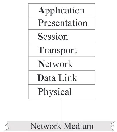
The OSI model, illustrated in Figure 2.1, is an architecture that divides network communication into seven layers, listed in the table below with a brief definition of the
functions that must be performed in a system for it to communicate. Each layer addresses a narrow portion of the communication process and covers different network activities,
equipment or protocols. For a detailed explanation of the functions of the various layers of
this model, refer to Tannenbaum (1989).
Table 2.1: Layers of the OSI Architecture
Layer Definition
1. Physical Layer Hardware Connections
2. Data Link Layer Coding, addressing, and transmitting information
3. Network layer Transport routes, message handling, and transfer
4. Transport layer Accurate delivery, service quality
5. Session layer Establishing, maintaining, and coordinating communication
6. Presentation layer Text formatting and display code
7. Application layer Program-to-program transfer of information
The packet creation process begins at the Application layer of the OSI model, where
the data is generated. Information to be sent across the network starts at the Application layer and goes through all seven layers (in the reverse order listed above). At each layer,
information relevant to that layer is added to the data. This information is for the
corresponding layer in the receiving machine. Information added to the Data Link Layer
in the sending computer, for instance, will be read by the Data Link layer in the receiving
computer.
The computer industry has designated several stacks as standard protocol models. The
most important ones include: the ISO/OSI protocol suite, the IBM Systems Network Architecture (SNA), Digital DECnet, Novell Netware, Apple AppleTalk, and the Internet
Figure 2.1: The Layers of the OSI Reference Model
2.6.2
Application Protocols
Application protocols work at the upper layer of the OSI model. They provide
application-to-application interaction and data exchange. More popular application protocols
in-clude: Advanced Program-to-Program Communication (APPC)—IBM’s peer-to-peer SNA
protocol; File Transfer Access and Management (FTAM)—an OSI file access protocol; X.400—a CCITT protocol for international e-mail transmissions; X.500—a CCITT protocol
for file and directory services across systems; Simple Mail Transfer Protocol (SMTP)—an
Internet protocol for transferring e-mail; File Transfer Protocol (FTP)—an Internet file transfer protocol; Simple Network Management Protocol (SNMP)— an Internet protocol for
monitoring networks and network components; TELNET—an Internet protocol for logging on to remote hosts and processing data locally; Microsoft Server Message Blocks (SMBs)
and client shells or redirectors; Novell Netware Core Protocol (NCP) and Novell client shells
or redirectors; AppleTalk and AppleShare—Apple’s networking protocol suite; AppleTalk Filing Protocol (AFP)—Apple’s protocol for remote file access; and Data Access Protocol
2.6.3
Transmission Control Protocol (TCP/IP)
The Internet Protocol (IP) is part of the TCP/IP protocol suite, and is the most
widely-used internetworking protocol. It is connectionless and was designed to handle the
interconnection of the vast number of WAN and LAN networks comprising the ARPANET. ARPANET is the creation of ARPA (now DARPA), the (Defense) Advanced Research
Projects Agency of the U.S. Department of Defense (Tannenbaum 1989, p. 35). Starting in the late 1960s, it began stimulating research on the subject of computer networks by
providing grants to computer science departments at many U.S. universities, as well as to
several corporations. Ultimately other networks, including BITNET, Usenet, UUCP, and NSFnet, were connected to ARPANET, which evolved into the Internet.
TCP/IP is an industry standard suite of protocols providing communications in a heterogeneous environment (Stallings 1997, pp. 520–525). In addition, TCP/IP provides a
routable, enterprise networking protocol and access to the Internet and its resources. Most Internet applications, such as World Wide Web and file transfer, use TCP. Because of its
popularity, TCP/IP has become the de facto standard for internetworking. Other protocols
written specifically for the TCP/IP suite include SMTP, FTP, and SNMP. TCP/IP has become the standard protocol used for interoperability among many different types of
computers. Historically, there were two primary disadvantages of TCP/IP: its size and speed. TCP/IP is a relatively large protocol stack which can cause problems in MS-DOS–
based clients. However, on graphical user interface (GUI)–based operating systems, such
as Windows NT or Windows 95, the size is not an issue and speed is about the same as Internetwork Packet Exchange (IPX). IPX is the NetWare protocol for packet forwarding
and routing. It is a relatively small and fast protocol on a LAN.
This chapter is a general overview of the various technologies involved in the traffic
process so as to provide some understanding of the complexity and diversity of computer networks. In view of the wide scope covered in this area, it has to be pointed out that our
research work will focus on packet transmissions pertaining to the LAN networks, and in
Chapter 3
Traffic Models and Statistical Analysis of Traffic
Data : A Literature Review
Sections 3.1–3.5 cover some basic definitions, and survey the current main traffic models found in the literature. The remaining part of this chapter reviews certain statistical tests
of the Hurst parameter (see§3.1.1 for the definition of the Hurst parameter) for long-range
dependent processes that have appeared in the literature. It will be seen that most of the
tests are based on the properties of LRD developed in §3.1.2. These tests were applied to
the Ethernet data from NC State University (called Dataset A); the results are discussed
in§3.8.
3.1
Preliminaries
In this section, the related concepts of self-similarity, long-range dependence, slowly
decaying variance, and the heavy-tailed property are considered. Our presentation is based
mostly on Cox (1984) and Beran (1992, 1994).
3.1.1
Self-Similarity
Self-similar processes and their corresponding increment processes were first introduced in statistics by Mandelbrot and co-workers (Mandelbrot and Van Ness 1968; Mandelbrot and
Wallis 1968a, 1969). For extensive surveys on self-similar processes, see Verwaat (1987) and
Let X ≡ {Xn : n ≥ 1} be a covariance stationary (sometimes called wide-sense
stationary (WSS)) stochastic process with mean µ = E[Xn], variance σ2=E[(Xn−µ)2],
and autocovariance function γq =E[(Xn−µ)(Xn+q−µ)], −∞< q <∞. The quantity γq
depends only on the lag q but not on the time n. Observe that σ2 = γ0. Denote rq the
process autocorrelation function at lag q, whererq≡γq/γ0. Here, Xn might represent the
number of packets, cells, or bytes that arrived during thenth time interval of sizeξ seconds.
Note thatXnis obtained by
Xn≡N(nξ)−N((n−1)ξ)
when it is constructed from the underlying counting process {N(t) : t ≥ 0}, where N(t)
records the number of arrivals by time t.
From the original process X defined above, one can define an aggregate WSS process
X(m) ≡ {Xk(m) : k ≥ 1}, obtained by averaging the Xn’s over adjacent, nonoverlapping
blocks of sizem, i.e.,
Xk(m)= 1
m(X(k−1)m+1+· · ·+Xkm).
The discrete-time process X = {Xn : n = 1,2, . . .} is said to be self-similar with
self-similarity parameterH if for any block sizem, the process{m1−HXk(m):k= 1,2, . . .}has
the same finite-dimensional distributions as X, i.e.,
{Xn:n= 1,2, . . .} d
={m1−HXk(m) :k= 1,2, . . .}. (3.1)
The processXissecond-order self-similar if for any block sizem, the process{m1−HX(m)
k :
k= 1,2, . . .}has the same covariance structure as X:
Var[m1−HXk(m)] = Var[Xn] = γ0
Corr[m1−HXk(m), m1−HXk(m+)q] = Corr[Xn, Xn+q] =rq, q= 1,2. . . .
)
(3.2)
In other words, the process {Xn} is exactly second-order self-similar if it satisfies (3.2) for
all aggregation levels m. It is said that {Xn} is asymptotically second-order self-similar if
(3.2) holds as m → ∞. An example of a self-similar process is fractional Gaussian noise
(FGN) with 1/2< H <1 (see§3.4.1).
3.1.2
Long-Range Dependence (LRD) and Slowly Decaying Variance
Let Var(Xk(m)) denote the variance of the above aggregated WSS process{Xk(m)}. Then
Var(Xk(m)) = σ
2 m +
2
m2
mX−1
q=1
Following the definition given in Cox (1984, pp. 57–58), we can distinguish two classes of
processes. The covariance stationary process {Xn : n ≥ 1} is said to have short-range
dependence (SRD) if
∞
X
q=−∞
|γq|<∞. (3.4)
In a process with SRD, note from (3.3) that for large m, Var(X(m)) is asymptotically of
the form v0/m, where v0 =P∞q=−∞γq is a finite process constant. The stationary process
{Xn :n≥1} is said to have LRD if
∞
X
q=−∞
|γq|=∞. (3.5)
A number of authors consider the following more restrictive definition for LRD. For
example, Beran (1992) defined a process {Xn :n≥1} to have LRD if its autocorrelation
function is of the form
rk∼k−(2−2H)L1(k) forklarge, (3.6)
where
0.5< H <1 (3.7)
and L1 is a slowly varying function at infinity, i.e.,
lim
t→∞L1(tx)/L1(t) = 1 for all x >0 (3.8)
(e.g., L1(t) equal to a constant, or L1(t) = logt). The symbol “∼” means asymptotic
equivalence.
Processes that have a steady-state distribution are often weakly dependent, in the
sense that observations that are far apart from each other in the sequence are almost
independent. Long-range dependent processes are thus considered as weakly dependent processes. However, the time-lag between two events must be very large for these events
to be almost statistically independent. This is in contrast to SRD processes, where the necessary time lag is relatively small.
The slowly decaying variance property can be mathematically expressed as
where a is a finite positive constant independent of m and β = 2−2H. For a process
with SRD, (3.9) holds withβ = 1 even though the self-similarity parameterH may not be
defined; and for a process with LRD, (3.6) implies that (3.9) holds with 0< β <1 so that
1/2< H <1. See Cox (1984) and Beran (1992, 1994) for details.
By slowing decaying variance, it is meant that the variance of the sample mean decreases
much more slowly than the reciprocal of the sample size. For short-range dependent
processes, the variance of a sample mean decreases as the reciprocal of the sample size,
and soβ = 1 in (3.9). On the other hand, a long-range dependent process is such that the
variance decreases more slowly than the reciprocal of the sample size. This property can be
detected by plotting Var(Xk(m)) againstm on a log-log plot, called variance-time plot (Fox
and Taqqu 1986). If this plot forms a straight line with a slope strictly between 0 and −1
over a wide range of m, then the process X is said to (or thought to) possess the slowly
decaying variance property.
3.1.3
Heavy-Tailed Distributions
While self-similarity concerns scaling properties of time-dependent statistics such as the
autocorrelation function, the heavy-tailed property is related to the marginal amplitude
distribution of Xn (Garrett 1994). A random variable U is said to be heavy-tailed if its
survivor or complementary distribution has the form
Pr{U ≥u} ∼u−α asu→ ∞ (3.10)
forα >0. A more general definition for heavy-tailed distribution is given by Resnick (1997),
where a heavy-tailed random variable U is such that Pr{U ≥u} ∼ u−αL(u), withL(u) a
slowly varying function at infinity. Of particular interest here is the case 1 < α <2, i.e.,
U has finite mean and infinite variance. Mandelbrot et al. (1968) refer to this property as
infinite variance syndrome or the Noah Effect. Intuitively, the infinite variance syndrome allows for compact descriptions of highly variable phenomena, i.e., random variables that
can take extreme values with nonnegligible probabilities, thus inducing LRD.
3.2
Early Traffic Models
The traditional models in traffic processes are renewal-based and Markov-based. Renewal models have a long history because of their relative mathematical simplicity. Poisson models
the telephone engineer A. K. Erlang. A Poisson process can be characterized as a renewal
process whose interarrival times {An : n ≥ 1} are exponentially distributed with rate
parameter λ, i.e., P{An ≤x}= 1−exp(−λx) for allx ≥0. Equivalently, it is a counting
process {N(t) : t ≥ 0} such that N(0) = 0 and it has independent increments with a
Poisson distribution (see Billingsley 1979, p. 260). These models have been widely used in queueing analysis due to the memoryless property inherent in the model which makes
certain analytical computations tractable. See C¸ inlar (1975) for a detailed discussion.
It has been widely recognized that traffic in packet networks is burstier, in the sense
of having extreme variability, than a Poisson process is. This has motivated the study of
more general arrival processes such as the Markov-based models. Unlike renewal traffic
models, Markov-based traffic models (C¸ inlar 1975) introduce dependence into the random
sequence {An:n≥1}, which enables such models to capture traffic burstiness (because of
the nonzero autocorrelations in{An:n≥1}). Consider a continuous-time Markov process
M ≡ {M(t) : t ≥ 0} with a discrete state space. In this case, M behaves as follows: it
stays in some stateifor an exponentially distributed holding time with parameter λi, which
depends on i alone; it then jumps to state j with probability pij. It then stays in state j
for an exponentially distributed holding time with parameter λj, and then makes another
transition and so on. In a simple Markov traffic model, each jump of the Markov process is
interpreted as signaling an arrival, so interarrival times are exponentially distributed with rate parameters depending upon the state from which the jump occurred. This results in
dependence among interarrival times as a consequence of the Markov property.
An extremely important class of Markovian traffic models is that of Markov-modulated models. The idea is to introduce an explicit notion of state into the description of a traffic
stream—an auxiliary Markov process is evolving in time and its current state controls
(modulates) the probability law of the traffic mechanism. Let M ≡ {M(t) : t ≥ 0} be a
continuous-time Markov process, with state space {1,2, . . . , κ}. Now assume that while
M is in statew, the probability law of traffic arrivals is completely determined by w, and
this holds for every 1 ≤ w ≤ κ. Note that when M undergoes a transition to, say, state
j, then a new probability law for arrivals takes effect for the duration of statej, and so
on. Thus, the probability law governing the arrival process is modulated by the state ofM
(such processes are also called doubly stochastic).
The most commonly used Markov-modulated model is the Markov-Modulated Poisson
Process (MMPP) model (see Fischer 1992, for example), which combines the simplicity of
the modulating (Markov) process with that of the modulated (Poisson) process. In this case,
to a Poisson process at rate λw. As the state changes, so does the rate. As a simple
example, consider a two-state MMPP model, where one state is an “ON” state with an
associated positive Poisson rate, and the other is an “OFF” state with associated rate zero (such models are also known as interrupted Poisson for obvious reasons). These models have
been widely used to model voice traffic sources (Heffes 1986); the “ON” state corresponds to a talk spurt (when the speaker emits sound), and the “OFF” state corresponds to a
silence (when the speaker pauses for a break).
3.3
Recent Developments in Traffic Measurements
Although the traffic models described earlier are still popular and widely used, extensive studies of traffic measurements from a wide variety of networks during the last seven to eight
years has shed much light into the arena of traffic modeling. It has been well-documented
that classical Markovian models are unable to account for LRD and self-similarity behavior
(see §3.1 for definitions) found in actual traffic traces. Even as early as 1980, the first
extensive measurement study on computer-generated packet networks by Shoch and Hupp (1980), where the performance of an experimental Ethernet system directly connecting over
120 hosts with 3 Mbps bandwidth was analyzed, revealed behavior inconsistent with the
Markovian assumption.
The growing interest in this area can be seen from the numerous traffic measurements
studies and modeling work. Many of these studies involved data sets that have become classical, such as:
(i) the investigation of ISDN traffic (16 Kbps) reported in Meier et al. (1991).
(ii) the series of articles reporting on detailed statistical analyses of high-resolution
Ethernet LAN (10 Mbps) traces (see Leland et al. (1993, 1994); Willinger et al. (1995, 1995b) and WAN traffic (see Pawlita (1988); Danzig et al. (1992); and Paxson and
Floyd (1995)).
(iii) the examination of traffic collected from working Common Channel Signaling (CCS)
subnetworks (56 Kbps) detailed in Duffy et al. (1994).
(iv) the various attempts for dealing with variable bit rate (VBR) video traffic (see Heyman et al. (1992); Garrett and Willinger (1994); Beran et al. (1995); and Huang et al.
Additional traffic studies can be found in Klivansky et al. (1994), who reported on traffic
collection and analysis efforts involving NSFnet WANs at Georgia Institute of Technology.
Other traffic investigations include Cinotti et al. (1994) and Grossglauser and Bolot (1996), where the former involves studies on a DQDB MAN network at the University of Pisa
and the latter reported studies on France Telecom/CNET. Analysis of traffic data for FASTPAC, an Australian high-speed data network, is reported in Addie, Zukerman and
Neame (1995). Nowadays, practically all deployed or planned ATM testbeds in the U.S. and Europe contain significant traffic-measurement components, which will result in extremely
high-volume data from “live” ATM networks within the next few years.
Although there have been many studies of LAN traffic since the early Ethernet measurements of Shoch and Hupp (1980), the emphasis has been on intermediate time scale
behavior or on user-oriented measures of behavior such as LAN throughput and delay. Meier et al. (1991) measured ISDN D-channel packet data from an office automation environment.
They discovered very high variability in the data (e.g., interarrival times of packets, number of successive packet arrivals in certain states) which cannot be adequately captured using
traditional packet traffic models but, instead, seems to be best described with the help
of heavy-tailed distributions of the form (3.10). These authors subsequently proposed an elaborate and highly parameterized model for the measured traffic.
Leland, Taqqu, Willinger, and Wilson (1993, 1994) analyzed Ethernet traffic
measurements taken from local area networks at the Bellcore Morristown Research and
Engineering Center. In sharp contrast to traditional traffic modeling assumptions, they
found that aggregate packet streams are statistically self-similar or fractal in nature;
i.e., actual network traffic looks the same when measured over time scales ranging from
milliseconds to seconds and minutes and beyond. They also showed that traffic smoothing will not occur either in time (i.e., the dependence characteristics of the traffic stream will
persist over the long-range) or in space (i.e., multiplexing many streams of this nature will
not result in a smoother aggregate stream).
In an earlier study, Leland and Wilson (1991) found extreme variability, and indices of
dispersion (see§3.4.3 for a precise definition) of the arrival rate which did not converge to
steady values with increasing sample sizes within the LANs. They also found burstiness
on all time scales over a range of six orders of magnitude, from milliseconds to days. This means that there was no natural time scale on which bursts were organized. They argued
that any feasible variant of traditional models would not show such features. The results
self-similar and exhibits LRD.
Similar findings were reported by Paxson and Floyd (1995) for WAN traffic
measurements. They evaluated 24 wide area traces, and showed that while Poisson-based traffic models were valid for modeling the arrival of user sessions, they did not suffice for
modeling most other WAN arrival processes. They found that the Poisson process was inadequate to capture the burstiness of the TELNET traffic. In this context, the observed
self-similar characteristic at the aggregate level can be directly related to high variability phenomena at the microscopic level, where in this case, microscopic level refers to the level
of the individual connections/applications that generate the overall traffic (e.g., WWW,
FTP, TELNET).
The importance of LRD in network traffic was first noted by Leland and Wilson (1991)
who showed that packet loss and delay behavior is radically different in simulations using real traffic data rather than traditional Markovian-based network models.
3.4
Self-Similar Traffic Models
These discoveries have invigorated research into new traffic models. The earliest of these
models is the “packet-train” model proposed by Jain and Routhier (1986). This model received significant attention, as its construction was based on the behavior of actual traces
and thus was consistent with traffic patterns. However, because of its lack of mathematical
representation, this model failed to explain how the model could yield such long-range behavior in traffic in a rigorous manner.
It was the extensive studies of Willinger et al. (1993, 1994, 1995b) that initiated a considerable body of research on the development of self-similar traffic models. Pursuing
an approach originally suggested by Mandelbrot (1965), these authors showed that the superposition of many ON/OFF sources, each of which exhibits the infinite variance
syndrome, results in self-similar aggregate traffic. They presented an idealized ON/OFF
source model which allows for long packet trains (“ON” periods, i.e., periods during which packets arrive at regular intervals) and long intertrain distances (“OFF” periods, i.e.,
periods with no packet arrivals). In their model, the ON- and OFF-periods did not strictly alternate (as is common in traditional communications literature): they were i.i.d. and
hence an ON-period could be followed by other ON-periods, and an OFF-period by other OFF-periods. For an extensive proof of the result, refer to Taqqu et al. (1997).
(also known as packet train models introduced by Jain and Routhier (1986)), the infinite
variance property of the distribution of the sojourn time in the ON and/or OFF state is
identified as the essential point of departure from traditional to self-similar traffic modeling. In this context, the infinite variance assumption of an individual ON/OFF source model
results in highly variable ON- and OFF-periods, i.e., the “train lengths” and “intertrain” distances can be very large with nonnegligible probability. These authors suggested the
use of the Hurst parameter as a measure of the degree of self-similarity of the aggregate traffic. The cited references also include a variety of statistical tests performed on the data
to estimate the Hurst parameter.
Even though independence governs the above description of the individual ON/OFF source model (i.e., the periods are i.i.d., the OFF-periods are i.i.d., and the
ON-and OFF-periods are independent from one another), an infinite-variance distribution for the sojourn time in the ON and/or OFF state can be readily shown to lead to
LRD in the stationary “reward” process corresponding to an individual ON/OFF source (e.g., a reward of one while in the ON state and a zero reward in the OFF-state). By
aggregating many such sources, the dependence structure remains unchanged, but the
marginal distribution becomes more Gaussian; finally, additional aggregation in time results in fractional Gaussian noise. In sharp contrast to these findings, traditional traffic modeling,
when cast in the framework of ON/OFF source models, without exception assumes finite-variance distributions for the ON- and OFF-periods (e.g., exponential distribution,
geometric distribution). These assumptions drastically limit the ON/OFF activities of an
individual source, and as a result, the superposition of many such sources behaves like white noise in the sense that the aggregate traffic stream is void of any significant correlations,
except possibly some in the short range.
Using actual traffic traces, Willinger et al. (1995b) have demonstrated that infinite
variance phenomena are in full agreement with measured network traffic. They revisited
the Bellcore Ethernet LAN traffic traces and extracted from the aggregate traffic the traces generated by individual source-destination pairs. Subsequent statistical analyses of these
traces revealed that (i) the traffic generated by individual source-destination pairs was
consistent with an ON/OFF model, and (ii) the distributions of the sojourn-times in the
ON/OFF states could be accurately described using Pareto-type distributions that exhibit infinite variance. The approach advocated by the Bellcore researchers is to regard
self-similar modeling as “parsimonious” in which the statistics of fluctuations are accounted for
in a stationary model, namely by fractional Gaussian noise (FGN) models and fractional
ARIMAprocesses. These two models are the best known examples of stationary stochastic