Multi-camera multi-object voxel-based Monte Carlo 3D tracking strategies

R E S E A R C H

Open Access

Multi-camera multi-object voxel-based Monte

Carlo 3D tracking strategies

Cristian Canton-Ferrer

, Josep R Casas, Montse Pardàs and Enric Monte

Abstract

This article presents a new approach to the problem of simultaneous tracking of several people in low-resolution sequences from multiple calibrated cameras. Redundancy among cameras is exploited to generate a discrete 3D colored representation of the scene, being the starting point of the processing chain. We review how the initiation and termination of tracks influences the overall tracker performance, and present a Bayesian approach to efficiently create and destroy tracks. Two Monte Carlo-based schemes adapted to the incoming 3D discrete data are

introduced. First, a particle filtering technique is proposed relying on a volume likelihood function taking into account both occupancy and color information. Sparse sampling is presented as an alternative based on a sampling of the surface voxels in order to estimate the centroid of the tracked people. In this case, the likelihood function is based on local neighborhoods computations thus dramatically decreasing the computational load of the algorithm. A discrete 3D re-sampling procedure is introduced to drive these samples along time. Multiple targets are tracked by means of multiple filters, and interaction among them is modeled through a 3D blocking scheme. Tests over CLEAR-annotated database yield quantitative results showing the effectiveness of the proposed algorithms in indoor scenarios, and a fair comparison with other state-of-the-art algorithms is presented. We also consider the real-time performance of the proposed algorithm.

1 Introduction

Tracking multiple objects and keeping record of their identities along time in a cluttered dynamic scene is a major research topic in computer vision, basically fos-tered by the number of applications that benefit from the retrieved information. For instance, multi-person track-ing has been found useful for automatic scene analysis [1], human-computer interfaces [2], and detection of unusual behaviors in security applications [3].

A number of methods for camera-based multi-person 3D tracking have been proposed in the literature [4-7]. A common goal in these systems is robustness under occlu-sions created by the multiple objects cluttering the scene when estimating the position of a target. Single-camera approaches [8] have been widely employed, but they are vulnerable to occlusions, rotation, and scale changes of the target. In order to avoid these drawbacks, multi-cam-era tracking techniques exploit spatial redundancy among different views and provide 3D information at the actual scale of the objects in the real world. Integration

of data extracted from multiple cameras has been pro-posed in terms of a fusion at feature level as image corre-spondences [9] or multi-view histograms [10] among others. Information fusion at data or raw level has been achieved by means of voxel reconstructions [11], polygon meshes [12], etc.

Most multi-camera approaches rely on a separate ana-lysis of each camera view, followed by a feature fusion process to finally generate an output. Exploiting the underlying epipolar geometry of a multi-camera setup toward finding the most coherent feature correspondence among views was first tackled by Mikičet al. [13] using algebraic methods together with a Kalman filter, and further developed by Focken et al. [14]. Exploiting epipo-lar consistency within a robust Bayesian framework was also presented by Canton-Ferrer et al. [9]. Other systems rely on detecting semantically relevant patterns among multiple cameras to feed the tracking algorithm as done in [15] by detecting faces. Particle filtering (PF) [16] has been a commonly employed algorithm because of its abil-ity to deal with problems involving multi-modal distribu-tions and non-linearities. Lanz et al. [10] proposed a multi-camera PF tracker exploiting foreground and color * Correspondence: [email protected]

Image and Video Processsing Group, Technical University of Catalonia, Barcelona, Spain

information, and several contributions have also followed this path: [4,7]. Occlusions, being a common problem in feature fusion methods, have been addressed in [17] using HMM to model the temporal evolution of occlu-sions within a PF algorithm. Information about the track-ing scenario can also be exploited toward detecttrack-ing and managing occlusions as done in [18] by modeling the occluding elements, such as furniture, in a training phase before tracking. It must be noted that, in this article, we assume that all cameras will be covering the area under study. Other approaches to multi-camera/multi-person tracking do not require maximizing the overlap of the field of view of multiple cameras, leading to the non-overlapped multi-camera tracking algorithms [19].

Multi-camera/multi-person tracking algorithms based on a data fusion before doing any analysis was pioneered by Lopez et al. [20] by using a voxelareconstruction of the scene. This idea was further developed by the authors in [5,21] finally leading to the present article. Up to our knowledge, this is the first approach to multi-person track-ing exploittrack-ing data fusion from multiple cameras as the input of the algorithms. In this article, we first introduce a methodology to multi-person tracking based on a colored voxel representation of the scene as the start of the pro-cessing chain. The contribution of this article is twofold. First, we emphasize the importance of the initiation and termination of tracks, usually neglected in most tracking algorithms, that has indeed an impact on the performance of the overall system. A general technique for the initia-tion/termination of tracks is presented. The second contri-bution is the filtering step where two techniques are introduced. The first technique applies PF to input voxels to estimate the centroid of the tracked targets. However, this process is far from real-time performance and an alternative, that we call Sparse Sampling (SS). SS aims at decreasing computation time by means of a novel tracking technique based on the seminal PF principle. Particles no longer sample the state space but instead a magnitude whose expectancy produces the centroid of the tracked person: the surface voxels. The likelihood evaluation rely-ing on occupancy and color information is computed on local neighborhoods, thus dramatically decreasing the computation load of the overall algorithm. Finally, effec-tiveness of the proposed techniques is assessed by means of objective metrics defined in the framework of the CLEAR [22] multi-target tracking database. Computa-tional performance is reviewed toward proving the real-time operation of the SS algorithms. Fair comparisons with state-of-the-art methods evaluated using the same database are also presented and discussed.

2 Tracker design methodology

Typically, a multi-target tracking system can be depicted as in Figure 1 and comprises a number of elementary

modules. Although most articles present techniques that contribute to filtering module, the overall architecture is rarely addressed assuming that some blocks are already available. In this section, this scheme will be analyzed and some proposals for each module will be presented. The filtering step, being our major contribution, will be addressed in a separate section.

2.1 Input and output data

When addressing the problem of multi-person tracking within a multi-camera environment, a strategy about how to process this information is needed. Many approaches perform an analysis of the images separately, and then combine the results using some geometric con-straints [10]. This approach is denoted as an information combination by fusion of decisions. However, a major issue in this procedure is dealing with occlusion and per-spective effects. A more efficient way to combine infor-mation is data fusion [23]. In our case, data fusion leads to a combination of information from all images to build up a new data representation, and to apply the algorithms directly on these data. Several data representations aggre-gating the information of multiple views have been pro-posed in the literature such as voxel reconstructions [11,24], level sets [25], polygon meshes [12], conexels [26], depth maps [27], etc. In our research, we opted for a colored voxel representation due to both its fast com-putation and accuracy.

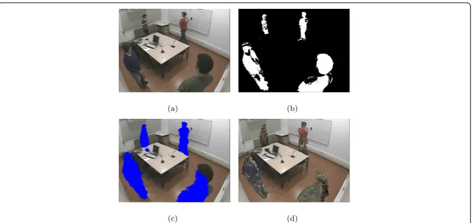
For a given frame in the video sequence, a set ofNC images are obtained from theNCcameras (see a sample in Figure 2(a)). Each camera is modeled using a pinhole camera model based on perspective projection with camera calibration information available. Foreground regions from input images are obtained using a segmen-tation algorithm based on Stauffer-Grimson’s back-ground learning and subtraction technique [28] as shown in Figure 2(b).

Redundancy among cameras is exploited by means of a Shape-from-Silhouette (SfS) technique [11]. This process generates a discrete occupancy representation of the 3D space (voxels). A voxel is labeled as foreground or back-ground by checking the spatial consistency of its projec-tion on the NC segmented silhouettes, and finally obtaining the 3D binary reconstruction shown in Figure 2(c). We will denote this raw voxel reconstruction asV. The visibility of a surface voxel onto a given camera is

Input Data

Tracker State Filter Analysis

Create track? Delete track?Analysis

Output

assessed by computing the discrete ray originating from its optical center to the center of this voxel using Bresen-ham’s algorithm and testing whether this ray intersects with any other foreground voxel. The most saturated color among pixels of the set of cameras that see a sur-face voxel is assigned to it. A colored representation of surface voxels of the scene is obtained, denoted as_VC_. An example of this process is depicted in Figure 2(d). It should be taken into account that, without loss of gener-ality, other background/foreground and 3D reconstruc-tion algorithms may be used to generate the input data to the tracking algorithm presented in this article.

The resulting colored 3D scene reconstruction is fed to the proposed system that assigns a tracker to each target and the obtained tracks are processed by a higher seman-tic analysis module. Information about the environment (dimensions of the room, furniture, etc.) allows assessing the validity of tracked volumes and discarding false volume detections.

Finally, the output of the overall tracking algorithm will be a number of hypotheses for the centroid position of each of the targets present in the scene.

2.2 Tracker state and filtering

One of the major challenges in multi-target tracking is the estimation of the number of targets and their posi-tions in the scene, based on a set of uncertain observa-tions. This issue can be addressed from two perspectives. First, extending the theory of single-target algorithms to multiple targets. This approach defines the working state space _X as the concatenation of the positions of allNT

targets asX = [x1,x2...xNT]. The difficulty here is the

time variant dimensionality of this space. Monte Carlo approaches, and specifically PF approaches, to this pro-blem have to face the exponential dependency between the number of particles required by the filter and the dimension of X, turning out to be computationally infeasible. Recently, a solution based on random finite sets achieving linear complexity has been presented [29].

Multi-target tracking can also be tackled by tracking each target independently, that is to maintainNT track-ers with a state space Xi=xi. In this case, the system attains a linear complexity with the number of targets, thus allowing feasible implementations. However, inter-actions among targets must be modeled in order to ensure the most independent set of tracks. This approach to multi-person tracking will be adopted in our research.

2.3 Track initiation and termination

A crucial factor in the performance of a tracking system is the module that addresses the initiation and termina-tion of tracks. The initiatermina-tion of a new tracker is inde-pendent of the employed filtering technique and only relies on the input data and the current state (position) of the tracks in the scene. On the other hand, the termi-nation of a new tracking filter is driven by the perfor-mance of the tracker.

The initialization of a new filter is determined by the correct detection of a person in the analyzed scene. This process is crucial when tracking, and its correct opera-tion will drive the overall system’s accuracy. However,

(a) (b)

(c) (d)

despite the importance of this step, little attention is paid to it in the design of multi-object trackers in the literature. Only few articles explicitly mention this pro-cess such as [30] that employs a face detector to detect a person or [31] that uses scout particle filters to explore the 3D space for new targets. Moreover, it is assumed that all targets in the scene are of interest, i.e., people, not accounting for spurious objects, i.e., furni-ture, shadows, etc. In this section, we introduce a method to properly handle the initiation and termina-tion of filters from a Bayesian perspective.

2.3.1 Track initiation criteria

The 3D input data V fed to the tracking system is usually corrupted and presents a number of inaccuracies such as objects not reconstructed, mergings among adja-cent blobs, spurious blobs, etc. Hence, defining a track initialization criterium based solely on the presence of a blob might lead to poor performance of the system. For instance, objects such as furniture might be wrongly detected as foreground, reconstructed and tracked. Instead, a classification of the blobs based on a probabil-istic criteria can be applied during this initialization pro-cess aiming at a more robust operation. Training of this classifier is based on the development set of the used database, together with the available ground truth describing the position of the tracked objects.

Let XGT=x1, ...,xNGT

be the ground truth positions of theNGTtargets present in the scene of the develop-ment set at a given instant. Once the reconstructionV is available, a connected component analysis is per-formed over these data thus obtaining a set ofKdisjoint components,Ci, fulfilling:

V=

K

i=1

Ci. (1)

We will consider the region of influence of a target with centroid xas the ellipsoid E(x,y) with axis size s = (sx,sy,sz) centered atc.

A mapping is defined such that for every xj Î XGTa componentCi is assigned. Let us denote [x]{x,y,z}as the x,y orzcoordinate of vector x. The assignation process is defined as follows: first, a region of influence E(xj,s) with sizes= (sx,sy, [xj]z) centered atc=xjis placed in

the 3D space. The radiisxandsyare chosen to contain

an average person, sx =sy= 30 cm. Let us define the

operator |·| applied to a volume as the number of non-zero voxels contained in it. Then, the assignation is defined as

xj→arg max i

_E(xj,s)∩Ci, ₍₂₎

that is to assign xj to the component with the largest volume enclosed in the region of influence. It must be noted that somexjmight not have anyCiassociated due to a wrong segmentation or faulty reconstruction of the target. Moreover, the set of components not associated to any ground truth position can be identified as spur-ious objects, reconstructed shadows, etc.

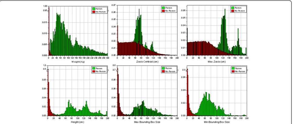
Finally, we have grouped the set of connected compo-nentsCiin two categories: person and non-person. A set of features are extracted from each of these compo-nents, thus conforming the characteristics that will be used to train a person/no-person binary classifier. This set of extracted features is described in Table 1.

In order to characterize the objects to be tracked and to decide the best classifier system, we have performed an exploratory data analysis [32], which will allow us to contrast the underlying hypotheses of the classifiers with the actual data. Histograms of these features are com-puted as shown in Figure 3 and scatter plots depicting the cross dependencies among all features are

Table 1 Features employed by the person/no-person classifier where magnitude[V]_{x,y,z}denotes thex,y, orz coordinates of voxelV

Feature Expression

Weight |C_i|_s3_vρ r= 1.1 [gr/cm3_]

Centroid (z-axis) |Ci|−1

v∈Ci

[V]z

Top max_V∈C

i

[V]z

Height max_V∈C

i

[V]z−max

V∈Ci

[V]z

Bounding box

max

max

V∈Ci

[V]_x−max

V∈Ci

[V]_x, max

V∈Ci

[V]_y−max

V∈Ci

[V]_y

min

max

V∈Ci

[V]_x−max

V∈Ci

[V]_x, max

V∈Ci

[V]_y−max

V∈Ci

computed. Observing Figure 3, we see that some vari-ables are easily separable, i.e., weight, height, and bounding box. Moreover, they show a low cross depen-dency with other features.

A number of standard binary classifiers has been tested and their performances have been evaluated, namely Gaussian, Mixture of Gaussians, Neural Net-works, K-Means, PCA, Parzen and Decision Trees [33,34]. Due to the aforementioned properties of the sta-tistic distributions of the features, some classifiers are unable to obtain a good performance, i.e., Gaussian, PCA, etc. Other classifiers require a large number of characterizing elements, such as K-Means, MoG, or Par-zen. Decision trees [33] have reported the best results. Separable variables such as height, weight, and bounding box size are automatically selected to build up a deci-sion tree that yields a high recognition rate with a preci-sion of 0.98 and a recall of 0.99 in our test database.

Another complementary criterium employed in the initiation of new tracks is based on the current state of the tracker. It will not be allowed to create a new track if its distance to the closest target is below a threshold.

2.3.2 Track termination criteria

A target will be deleted if one of the following condi-tions is fulfilled:

- If two or more tracks fall too close to one another, this indicates that they might be tracking the same target, hence only one will be kept alive while the rest will be removed.

- If tracker’s efficiency becomes very low it might indicate that the target has disappeared and should be removed.

- The person/no-person classifier is applied to the set of features extracted from the voxels assigned to a target. If the classifier outputs a no-person verdict for a number of frames, the target will be considered as lost.

3 Voxel-based solutions

The filtering block shown in Figure 1 addresses the pro-blem of keeping consistent trajectories of the tracked objects, resolving crossings among targets, mergings with spurious objects (i.e., shadows) and producing an accurate estimation of the centroid of the target based on the input voxel information. Although there is a number of papers addressing the problem of multi-cam-era/multi-person tracking, very few contributions have been based on voxel analysis [20,21].

3.1 PF tracking

PF is an approximation technique for estimation pro-blems where the variables involved do not hold Gaus-sianity uncertainty models and linear dynamics. The current tracking scenario can be tackled by means of this algorithm to estimate the 3D position of a personxt = (x, y, z)t at time t, taking as observation a set of

colored voxels representing the 3D scene up to timet denoted as z1:t. For a given targetxt, PF approximates

the posterior density p(xt|z1:t) as a sum of Np Dirac functions:

p(xt|z1:t)≈

Np

j=1

wjtδ(xt−xjt), (3)

where wjt are the weights associated to the particles,

fulfilling _jwjt= 1, and xjt their positions. For this type of tracking problem, a sampling importance re-sampling (SIR) PF is applied to drive particles along time [16]. Assuming importance density to be equal to the prior density, weight update is recursively computed as

wjt∝w j t−1p

zt|xjt

. (4)

SIR PF avoids the particle degeneracy problem by re-sampling at every time step. In this case, weights are set to wj_t−1=N−_P1, ∀j; therefore,

wjt∝p

zt|xjt

. (5)

Hence, the weights are proportional to the likelihood function that will be computed over the incoming volumezt.

Finally, the best state at timet, x˜t, is derived based on the discrete approximation of Equation 3. The most common solution is the Monte Carlo approximation of the expectation as

˜

xt=E[xt|z1:t]≈ NP

j=1 wjtx

j

t. (6)

Basically, in the PF operation loop two steps must be defined: likelihood evaluation and particles propagation. In the following, we present our proposal for the PF implementation.

3.1.1 Likelihood evaluation

Binary and color information contained in zt will be

employed to define the likelihood function p

zt|xjt

relating the observation zt with the human body instance given by particle xjt, 1≤j≤NP. Two partial

likelihood functions, pRaw

Vt|xjt

and pColor

VC t|x

j t

,

will be combined linearly to produce pzt|xjt

as:

p

zt|xjt

=λpRaw

Vt|xjt

+ (1−λ)pColor

VC t|x

j t

. (7)

Factor l controls the influence of each term (fore-ground and color information) in the overall likelihood function. Empirical tests have shown thatl = 0.8 pro-vides satisfactory results. A more detailed review of the impact of color information in the overall performance of the algorithm is addressed in Section5.1.

Likelihood associated to raw data is defined as the ratio of overlap between the input dataVtand the ellip-soid _Ej

t defined by particle x j

t (see Section 2.3.1)

as

pRaw

Vt|xjt

=

Vt∩Etj

Ej

t

. (8)

For a given target k, an adaptive reference histogram

Hk_t of the colored surface voxels is available. This histo-gram is constructed using the YCbCr color space due to its robustness against light variations. The number of bins per channel will drive the ability of the system to distinguish between different color blobs; for our experi-ments, 21 bins per channel have been set empirically. The color likelihood function is constructed as

pColor

VC t|x

j t

=BHk_t,HVC_t ∩Etj

, (9)

whereB(·) is the Bhattacharya distance andH(·) stands for the color histogram extraction operation of the enclosed volume. Update of the reference histogram is performed in a linear manner following the rule:

Hk_t =αHk_t−1+ (1−α)HVC_t ∩E_tx˜, (10)

where Ex˜

t stands for the ellipsoid placed in the cen-troid estimation x˜t and ais the adaptation coefficient. In our experiments,a= 0.9 provided satisfactory results.

3.1.2 Particle propagation

The propagation model has been chosen to be a Gaus-sian noise added to the state of the particles after the re-sampling step: xj_t+1=xjt+N. The covariance matrixP corresponding to N is proportional to the maximum variation of the centroid of the target and this informa-tion is obtained from the development part of the test-ing dataset. More sophisticated schemes employ previously learnt motion priors to drive the particles more efficiently [6]. However, this would penalize the efficiency of the system when tracking unmodeled motions patterns and, since our algorithm is intended for any motion tracking, no dynamical model is adopted.

3.1.3 Interaction model

Hence, blocking information can also be considered when computing the particle weights for the kth target as

wkt,j=p

zt|xkt,j

NT

l=1

l=k

φx˜k_t−1,x˜l_t−1, ₍₁₁₎

where x_˜k_t−1 stands for the estimation of the PF at time t- 1 for targetkandj(·) is the blocking function defin-ing exclusion zones that penalize particles from target l falling into the exclusion zone of targetk. In this parti-cular case, considering that people in the room are always sitting or standing up, this zone can be con-strained to thexyplane. The proposed function is

φx˜k_t−1,x˜l_t−1= 1−exp

−kx˜k_t x,y−

˜

xl_t x,y

2

, (12)

where k∝s−2

x is the parameter that drives the sensi-bility of the exclusion zone.

3.2 SS tracking

In the presented PF tracking algorithm, likelihood eva-luation can be computationally expensive, thus render-ing this approach unsuitable for real-time systems. Moreover, data are usually noisy and may contain merged blobs corresponding to different targets. A new technique, SS, is proposed as an efficient and flexible alternative to PF.

Assuming a homogeneous 3D object, it can be proved that its centroid can exactly be computed based only on the surface voxels, since the interior voxels do not pro-vide any relevant information. Hence, this centroid can be estimated through a discrete version of Green’s theo-rem on the surface voxels [35,36], while other approaches obtain an accurate approximation of the centroid using feature points (see [37] for a review). A common assumption of these techniques is the

availability of surface data extracted beforehand, hence a labeling of the voxels in the scene should be available. By assuming that the object under study presents a cen-tral symmetry in thexy plane, the computation of the centroid can be done as an average of the positions of the surface voxels:

˜

xt = V∈V

t

[V]_x

|Vt|

= V∈V s

t

[V]_{x V}s

t

. (13)

3.2.1 Degree of mass and degree of surfaceness

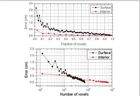
Let us model the human body as an ellipsoid as pre-viously done in the PF approach. In order to test the robustness of the centroid computation of Equation13 against missing data, we studied the error committed when only a fraction of these input data is employed. A number of voxels (surface or interior voxels in each case) is randomly selected and employed to compute the centroid. Then, the error is computed showing that the surface-based estimation is more sensitive than the estimation using interior voxels (see Figure 5). However, this proves that the centroid can be computed from a number of randomly selected surface voxels still achiev-ing a satisfactory performance. This idea is the underly-ing principle of the SS algorithm.

Let us estimate the centroid of an object by analyzing a randomly selected number of voxels from the whole scene, denoted asW. An approach to the computation of the centroid would be

˜

xt≈W∈Wt

ρ(W)[W]_x

W∈Wt

ρ(W) , ρ(W) =

1 ifW ∈Vt 0 ifW ∈Vt ,(14)

where ρ(W) gives the mass density of voxel W. Since it is assumed that all voxels have the same mass, this is a binary function that checks the occupancy of a given voxel. Hence, only the fraction of (randomly selected) voxels inside the object will contribute to the computation of the centroid. Equation14 can be rewrit-ten as

˜

xt≈

W∈Wt

ρ(W)

W∈Wt

ρ(W)[W]x=

W∈Wt

˜

ρ(W)[W]x,₍₁₅₎

where ρ˜(W) can be considered as the normalized mass contribution of voxel _W to the computation of the centroid. If function ρ(W) takes values in the range [0,1] we may consider it as the“degree of mass” ofW or the importance of voxel W into the calculation of x˜t. Then, ρ(W) might be considered as a normalized weight assigned toW. Since we stated that the centroid

(a) (b)

can be computed using surface voxels, Equation13 can be also posed as

˜

xt≈

W∈Wt

ρs(W)

W∈Wt

ρ(W)[W]x=

W∈Wt

˜

ρs(W)[W]x,₍₁₆₎

where ρs(W)∈[0, 1] measures the“degree of surface-ness” of voxelW. Within this context, functions r(·)

and rS(·) might be understood as pseudo-likelihood

functions and Equations 16 and 15 as a sample-based representation of an estimation problem.

3.2.2 Difference with particle filters

There is an obvious similarity between these representa-tion and the formularepresenta-tion of particle filters but there is a significant difference. While particles in PF represent an instance of the whole body, our samples(W∈Wt)are points in the 3D space. Moreover, particle likelihoods are computed over all data while sample pseudo-likeli-hoods will be computed in a local domain.

The presented concepts are applied to define the SS algorithm. Let yit∈R3, a point in the 3D space and ωi

t∈R its associated weight measuring the

pseudo-likelihood of this position being part of the object or part of its surface. Under certain assumptions, it is achieved that the centroid can be computed as

˜

xt ≈ Ns

i=1

ωi

tyit, (17)

where Ns is the number of sampling points. When using SS we are no longer sampling the state space since yi

tcannot be considered an instance of the cen-troid of the target as happened with particles, xjt, in PF. Hence, we will talk about samples instead of particles and we will refer to(yi

t,ωit)

Ns

i=1as the sampling set.

This set will approximate the surface of the kth target, VS,k_{, and will fulfill the sparsity conditionNs} VS,k_..

4 SS implementation

In order to define a method to recursively estimate x˜t from the sampling set(yi_t,ωit)

Ns

i=1, a filtering strategy

and estimation) with some opportune modifications to ensure the convergence of the algorithm.

4.1 Pseudo-likelihood evaluation

Associated weight wjt to a sample yit will measure the likelihood of that 3D position to be part of the surface of the tracked target. When computing the pseudo-like-lihood, surface has been chosen instead of interior vox-els, based on the efficiency of surface samples to propagate rapidly as will be explained in the next sec-tion. As in the defined PF likelihood function, two par-tial pseudo-likelihood functionsb, pRaw

Vt|yit

and pColor

VC t|yit

, are linearly combined to form pzt|yit

as

pzt|yit

=λpRaw

Vt|yit

+ (1−λ)pColor

VC t|yit

. (18)

Partial likelihoods will be computed on a local domain centered in the positionyi

t. Let C

yi t,q,r

be a neighbor-hood of radiusr over a connectivityqdomain on the 3D orthogonal grid around a sample place in a voxel posi-tion yi_t. Then, we define the occupancy and color neigh-borhoods around yi

t as Oit =Vt∩C

yi_t,q,r and

Ci_t =VC_t ∩Cyi_t,q,r, respectively. For a given sample yi

t occupying a single voxel, its weight associated to the raw data will measure its likeli-hood to belong to the surface of an object. It can be modeled as

pRaw

Vt|yit

= 1−

2Oi t

_C

yit,q,r

−1

. (19)

Ideally, when the sampleyi

t is placed in a surface, half of its associated occupancy neighborhood will be occu-pied and the other half empty. The proposed expression attains its maximum when this condition is fulfilled.

Function pColor

VC t|yit

can be defined as the likeli-hood of a sample belonging to the surface correspond-ing to the kth target characterized by an adaptive reference color histogram Hk_t:

pColor

VC t|yit

=DHk_t,Cjt

. (20)

Since Cjt contains only local color information with

reference of the global histogram Hk_t, the distanceD(·) is constructed toward giving a measure of the likelihood between this local colored region and Hk

t. For every

voxel in Cjt, it is decided whether it is similar to H m t by selecting the histogram value for the tested color and checking whether it is above a threshold g or not. Finally, the ratio between the number of similar color and total voxels in the neighborhood gives the color

similarity score. Since reference histogram is updated and changes over time, a variable threshold gis com-puted, so that the 80% of the values of Hm

t are taken into account.

One of the advantages of the SS algorithm is its com-putational efficiency. The complexity to compute

pzt|yit

is quite reduced since it only evaluates a local neighborhood around the sample in comparison with the computational load required to evaluate the likeli-hood of a particle in the PF algorithm. This point will be quantitatively addressed in Section5.2.

The parameters defining the neighborhood were set to q = 26 andr = 2 yielding to satisfactory results. Larger values of the radiusr did not significantly improve the overall algorithm performance but increased its compu-tational complexity.

4.2 Sample propagation and 3D discrete resampling

A sample yi

t placed near a surface will have an asso-ciated weight _ωj_t with a high value. It is a valid assump-tion to consider that some surrounding posiassump-tions might also be part of this surface. Hence, placing a number of new particles in the vicinity of xjt would contribute to progressively explore the surface of a voxel set. This idea leads to the spatial re-sampling and propagation scheme that will drive samples along time in the surface of the tracked target.

Given the discrete nature of the 3D voxel space, it will be assumed that every sample is constrained to occupy a single voxel or discrete 3D coordinate and there can-not be two samples placed in the same location. Re-sampling is mimicked from PF so a number of replicas proportional to the normalized weight of the sample are generated. Then, these new samples are propagated and somediscrete noise is added to their position meaning that their new positions are also constrained to occupy a discrete 3D coordinate (see an example in Figure 6). However, two re-sampled and propagated particles may

(a) (b)

fall in the same 3D voxel location as shown in Figure 6. In such case, one of these particles will randomly explore the adjacent voxels until reaching an empty location; if there is not any suitable location for this par-ticle, it will be dismissed.

The choice of sampling the surface voxels of the object instead of its interior voxels to finally obtain its centroid is motivated by the fact that propagating sam-ples along the surface rapidly spread them all around the object as depicted in Figure 7. Propagating samples on the surface is equivalent to propagate them on a 2D domain, hence the condition of not placing two samples in the same voxel will make them to explore the surface faster (see Figure 6). On the other hand, interior voxels propagate on a 3D domain, thus having more space to explore and therefore becoming slower to spread all around the volume (see Figure 6). Although both (pseudo-)likelihoods should produce a fair estimation of the object’s centroid, both sampling sets must fulfill the condition to be randomly spread around the object volume, otherwise the centroid estimation will be biased.

4.2.1 Interaction model

The flexibility of a sample-based analysis may, sometimes, lead to situations where particles spread out too much from the computed centroid. In order to cope with this problem, a intra-target samples’ interaction model is devised. If a sample is placed in a position such that

yi

t

x,y−

˜

xt−1

x,y> δ it will be removed (that is to

assignωi

t = 0) and we set the threshold asδ=asx, withsx

= 30 cm. Factora= 1.5 produced accurate results in our experiments.

The interaction among targets is modeled in similar way as in the PF approach. Formulas in Equations 11 and 12 are applied to samples with the appropriate scal-ing parameterk.

5 Results and evaluation

In order to assess the performance of the proposed track-ing systems, they have been tested on the set of

benchmarking image sequences provided by the CLEAR Evaluation Campaigns 2007 [22]. Typically, these evalua-tion sequences involved up to five people moving around in a meeting room. This benchmarking set was formed by two separate datasets, development, and evaluation, containing sequences recorded by five of the participating partners. A sample of these data can be seen in Figure 8. The development set consisted in 5 sequences of an approximate duration of 20 min each, while the evalua-tion set was formed by 40 sequences of 5min each, thus adding up to 5 h of data. Each sequence was recorded with four cameras placed in the corners of the room and a zenithal camera placed in the ceiling. All cameras were calibrated and had resolutions ranging from 640 × 480 to 756 × 576 pixels at an average frame rate offR= 25fps. The test environments were a 5 × 4 m rooms with occluding elements such as tables and chairs. Images of the empty rooms were also provided to train the back-ground/foreground segmentation algorithms.

Metrics proposed in [4] for multi-person tracking eva-luation have been adopted, namely the Multiple Object Tracking Precision (MOTP), which shows tracker’s abil-ity to estimate precise object positions, and the Multiple Object Tracking Accuracy (MOTA), which expresses its performance at estimating the number of objects, and at keeping consistent trajectories.MOTP scores the aver-age metric error when estimating multiple target 3D centroids, while MOTA evaluates the percentage of frames where targets have been missed, wrongly detected or mismatched.

The aim of a tracking system would be to produce high values of MOTA and low values of MOTP thus indicating its ability to correctly track all targets and estimate their positions accurately. When comparing two algorithms, there will be a preference to choose the one outputting the highest MOTA score.

5.1 Results

To demonstrate the effectiveness of the proposed multi-person tracking approaches, a set of experiments were

(a) Reference (b) Interior based likelihood (c) Surface based likelihood

conducted over the CLEAR 2007 database. The develop-ment part of the dataset was used to train the initiation/ termination of tracks modules as described in Section 2.3 and the remaining test part was used for our experiments.

First, the multi-camera data are pre-processed per-forming the foreground and background segmentations and 3D voxel reconstruction algorithm. In order to ana-lyze the dependency of the tracker’s performance with the resolution of the 3D reconstruction, several voxel sizes were employed sv ={2, 5, 10, 15} cm. A colored version of these voxel reconstructions was also gener-ated, according to the technique introduced in Section 2.1. Then, these data were the input fed to the PF and SS proposed approaches.

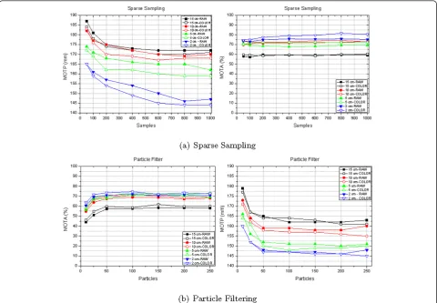
In both types of filters, SS or PF, three parameters drive the performance of the algorithm: the voxel size sv, the number of samplesNs, or particlesNp, and the usage of color information. Experiments carried out explore the influence of these parameters in the MOTP, precision in cm., and MOTA, tracker accuracy (in % of

correctly tracked targets), shown in Figure 9. Some remarks can be drawn

- Number of samples/particles: There is a depen-dency between the MOTP score and the number of par-ticles/samples, especially for the SS algorithm. The contribution of a new sample to the estimation of the centroid in the SS has less impact than the addition of a new particle in the PF, hence the slower decay of the MOTP curves for the SS than for the PF. Regarding the MOTA score, there is not a significant dependency with NsorNp. Two factors drive the MOTA of an algorithm: the track initiation/termination modules, that mainly contributes to the ratio of misses and false positives, and the filtering step that has an impact to the mis-matches ratio. The low dependency of MOTA with Ns orNpshows that most of the impact of the algorithm in this score is due to the particle/sample propagation and interaction strategies rather than the quantity of parti-cles/samples itself. Moreover, the influence in the MOTA score is tightly correlated with the track initia-tion/termination policy. This assumption was experi-mentally validated by testing several classification methods (mixture of Gaussians, PCA, Parzen, and K-Means) in the initiation/termination modules yielding to a drop in the MOTA score proportional to their ability to correctly classify a blob as person/no-person.

- Voxel size: Scenes reconstructed with a large voxel size do not capture well all spatial details and may miss some objects thus decreasing the performance of the system (both in SS and PF). It can be observed that MOTP and MOTA scores improve as the voxel size decrease.

-Color features: Color information improves the per-formance of SS and PF in both MOTP and MOTA scores. First, there is an improvement when using color information for a given voxel size, specially for the SS algorithm. Moreover, the smaller the voxel size the most noticeable difference between the experiments using raw and color features. This effect is supported by the fact that color characteristics are better captured when using small voxel sizes. The performance improvement when using color in the SS algorithm is more noticeable since samples are placed in the regions with a high likelihood to be part of the target. For instance, this effect is more evident in cases where the subject is sitting and the par-ticles concentrate in the upper body part, disregarding the part of the chair. In the SS algorithm, MOTP score benefits from this efficient sample placement. PF algo-rithm is constrained to evaluate the color likelihood in the ellipsoid defined in Equation 9 thus not being able to differentiate between parts of the blob that do not belong to the tracked target. Color information used within the filtering loop leads to a better distinguishabil-ity among blobs, thus reducing the mismatch ratio and

(a) (b)

(c) (d)

(e)

slightly improving the MOTA score. Merging of adja-cent blobs or complex crossing among targets is also correctly resolved. An example of the impact of color information is shown in Figure 10 where the usage of color avoids the mismatch between two targets. This effect is more noticeable when targets in the scene are dressed in different colors.

We can compare the results obtained by SS and PF with other algorithms evaluated using the same CLEAR 2007 database whose scores are reported in Table 2. Most of these methods exploited multi-view information with the exception of [31] that only used the zenithal camera facing the associated distortion and perspective problems. PF is the most employed technique due to its suitability to the characteristics of this problem although Kalman filtering used by [15] provided fair results when fed by higher semantical features extracted from the input data (in this case, faces). Note the lowFP score for this system as a consequence of the unlikely event of detecting a face in a spurious object. A 3D voxel recon-struction was used as the input data in [5] together with a simple track management system. The rest of the

methods [7,31] relied on a fixed human body appear-ance model similar to the ellipsoidal region of interest used in our PF proposal. However, the novelty of these Figure 9MOTP and MOTA scores for the SS and the PF techniques using raw and colored voxels. Several voxel sizessv= {2, 5, 10, 15} cm have been used in the experiments.

t t+ 1 t+ 2

Raw features

Color features

methods is the strategies to combine the information coming from the analysis of different views without per-forming any 3D reconstruction. Comparing the best

proposed tracking system [31]c with our two

approaches, we obtain a relative improvement of Δ (MOTP, MOTA)ss = (7.63,17.13)% and Δ(MOTP, MOTA)PF= (5.16,7.15)%.

In order to visually show the performance of the SS algorithm, some videos corresponding to the most chal-lenging tracking scenarios have been made available at http://www.cristiancanton.org.

5.2 Computational performance

Comparing obtained metrics among different algorithms can give an idea about their performance in a scenario where computational complexity is not taken into account. An analysis of the operation time of several algorithms under the same conditions and the produced MOTP/MOTA metrics might give a more informative and fairer comparison tool. Although there is not a standard procedure to measure the computational per-formance of a tracking process, we devised a method to assess the computational efficiency of our algorithms to present a comparative study.

The RTFfactor associated with a performance measure MOTP/MOTA (in both vertical axes) of the SS and PF algorithms when dealing with raw and colored input voxels is presented in Figure 11. This factor indicates a proportional measure of the speed of the algorithm whereRTF= 1 stands for real-time operation whileRTF > 1 and RTF < 1 indicate a faster or slower perfor-mance, respectively. Each point of every curve is the result of an experiment conducted over all the CLEAR data set associated to a number of samples/particles of each algorithm.

The first noticeable characteristic of these charts is that, due to the computational complexity of each algo-rithm, when comparing SS and PF algorithms under the same operation conditions, the RTF associated with SS

Figure 11Computational performance comparison between PF and SS using several voxel sizess_V ={2, 5, 10, 15}cmand features (raw or colored voxels). MOTP and MOTA scores are related to the real-time factor (RTF) showing the computational load required by each algorithm to attain a given tracking performance.

Table 2 Results presented at the CLEAR 2007 [22] by several partners

Method MOTP MOTA FP Miss MM

(mm) (%) (%) (%) (cases)

Face detection+Kalman filtering [15]

91 59.66 06.99 30.89 2.46

Appearance models+PF [7] 141 59.62 18.58 20.66 1.14

Upper body detection+PF [31] 155 69.58 14.50 15.09 0.83

Zenithal camera analysis+PF [31] 222 54.94 20.24 23.74 1.08

Voxel analysis+Heuristic tracker [5]

168 30.49 40.19 27.74 1.58

Voxel analysis+PF (best case) 147 74.56 14.03 10.48 0.91

Voxel analysis+SS (best case) 144 81.50 09.34 08.70 0.46

is always higher than the associated with PF. Similarly, the computational load is higher when analyzing colored than raw inputs. All the plotted curves attain lower RTF performance values as the size of the voxel sv decreases since the amount of data to process increases (note the different RTF scale ranges for each voxel size in Figure 11). Regarding the MOTP/MOTA metrics, there is a common tendency to a decrease in the MOTP and an increase in the MOTA as the RTF decreases. The separation between the SS and PF curves is bigger as the voxel size decreases since the PF algorithm has to evaluate a larger amount of data.

The observation of these results yields the conclusion that the SS algorithm is able to produce a similar and, in some cases, better results than the PF algorithm with a lower computational cost. For example, using sv = 5 cm, a MOTP score of around 165 mm can be obtained using SS with a RTF ten times larger than when using PF and similarly with the MOTA score.

6 Conclusions

In this article, we have presented a number of contribu-tions to the multi-person tracking task in a multi-cam-era environment. A block representation of the whole tracking process allowed to identify the performance bottlenecks of the system and address efficient solutions to each of them. Real-time performance of the system was a major goal hence efficient tracking algorithms have been produced as well as an analysis of their performance.

The performance of these systems has thoroughly been tested over the CLEAR database and quantitatively compared through two scores: MOTP and MOTA. A number of experiments have been conducted toward exploring the influence of the resolution of the 3D reconstruction and the color information. Results have been compared with other state-of-the-art algorithms evaluated with the same metrics using the same testing data.

The relevance of the initiation and termination of fil-ters have been proved, since these modules have a major impact on the MOTA score. However, most arti-cles in the literature do not specifically address the operation of these modules. We proposed a statistical classifier based on classification trees as a way to discri-minate blobs between the person/no-person classes. Training of this classifier was done using data available in the development part of the employed database and a number of features (namely weight, height, top inz-axis, bounding box size) were extracted and provided as the input to the classifier. Another criterium such as a proximity to other already existing tracks was employed to create or destroy a track. Performance scores in Table 2 for the PF and SS systems present the lowest

values for the false positives (FP) and missed targets (Miss) ratios hence supporting the relevance of the initiation and termination of tracks modules.

Two proposals for the filtering step of the tracking system have been presented: PF and SS. An independent tracker was assigned to every target and an interaction model was defined. PF technique proved to be robust and leaded to state-of-the-art results but its computa-tional load was unaffordable for small voxel sizes. As an alternative, SS algorithm has been presented achieving a similar and, in some occasions, better performance than PF at a smaller computational cost. Its sample-based estimation of the centroid allowed a better adaptation to noisy data and distinguishability among merged blobs. In both PF and SS, color information provided a useful cue to increase the robustness of the system against track mismatches thus increasing the MOTA score. In the SS, color information also allowed a better place-ment of the samples allowing to distinguish among parts belonging to the tracked object and parts of a merging with a spurious object, leading to a better MOTP score.

Future research within this topic involves multi-modal data fusion with audio data toward improving the preci-sion of the tracker, MOTP, and avoid mismatches among targets, thus improving the MOTA score.

End notes a

Analogously to the pixel definition (picture element) as the minimum information unit in a discrete image, the voxel (volume element) is defined as the minimum infor-mation unit in a 3D discrete representation of a volume.

b

For the sake of simplicity in the notation, pseudo-likelihood functions will be denoted as p(·) instead of defining a specific notation for it.

c

When selecting the best system, the MOTA score is regarded as the most significant value.

The authors declare that they have no competing interests

Received: 15 May 2011 Accepted: 23 November 2011 Published: 23 November 2011

References

1. S Park, MM Trivedi, Understanding human interactions with track and body synergies captured from multiple views. Comput Vis Image Understand

111(1), 2–20 (2008). doi:10.1016/j.cviu.2007.10.005

2. Project CHIL–Computers in the Human Interaction Loop, http://chil.server. de (2004–2007)

3. I Haritaoglu, D Harwood, LS Davis,W4_{: real-time surveillance of people and} their activities. IEEE Trans Pattern Anal Mach Intell.22(8), 809_–830 (2000). doi:10.1109/34.868683

4. K Bernardin, A Elbs, R Stiefelhagen, Multiple object tracking performance metrics and evaluation in a smart Room environment, inProceedings of IEEE International Workshop on Visual Surveillance(2006)

Relationships Evaluation and Workshop, vol. 4625. Lecture Notes on Computer Science, 91_–103 (2007)

6. Z Khan, T Balch, F Dellaert, Efficient particle filter-based tracking of multiple interacting targets using an MRF-based motion model, inProceedings of International Conference on Intelligent Robots and Systems.1(1), 254–259 (2003)

7. O Lanz, P Chippendale, R Brunelli, An appearance-based particle filter for visual tracking in smart rooms, inProceedings of Classification of Events, Activities and Relationships Evaluation and Workshop, vol. 4625. Lecture Notes on Computer Science, 57–69 (2007)

8. A Yilmaz, O Javed, M Shah, Object tracking: a survey. ACM Comput Surv.

38(4), 1–45 (2006)

9. C Canton-Ferrer, JR Casas, M Pardàs, Towards a Bayesian approach to robust finding correspondences in multiple view geometry environments, inProceedings of 4th International Workshop on Computer Graphics and Geometric Modelling, vol. 3515. Lecture Notes on Computer Science, 281_–289 (2005)

10. O Lanz, Approximate Bayesian multibody tracking. IEEE Trans Pattern Anal Mach Intell.28(9), 1436–1449 (2006)

11. GKM Cheung, T Kanade, JY Bouguet, M Holler, A real time system for robust 3D voxel reconstruction of human motions, inIEEE Conference on Computer Vision and Pattern Recognition2, 714_–720 (2000)

12. J Isidoro, S Sclaroff, Stochastic refinement of the visual hull to satisfy photometric and silhouette consistency constraints, inProceedings of IEEE International Conference on Computer Vision2, 1335–1342 (2003) 13. I Miki_č, S Santini, R Jain, Tracking objects in 3D using multiple camera

views, inProceedings of Asian Conference on Computer Vision(2000) 14. D Focken, R Stiefelhagen, Towards vision-based 3-D people tracking in a

Smart Room, inProceedings of IEEE International Conference on Multimodal Interfaces, 400–405 (2002)

15. N Katsarakis, F Talantzis, A Pnevmatikakis, L Polymenakos, The AIT 3D audiovisual person tracker for CLEAR 2007, inProceedings of Classification of Events, Activities and Relationships Evaluation and Workshop, vol. 4625. Lecture Notes on Computer Science, 35–46 (2007)

16. MS Arulampalam, S Maskell, N Gordon, T Clapp, A tutorial on particle filters for online nonlinear/non-Gaussian Bayesian tracking. IEEE Trans Signal Process.50(2), 174_–188 (2002). doi:10.1109/78.978374

17. K Lien, C Huang, Multiview-based cooperative tracking of multiple human objects. EURASIP J. Image Video Process8(2), 1–13 (2008)

18. T Osawa, X Wu, K Sudo, K Wakabayashi, H Arai, MCMC based multi-body tracking using full 3D model of both target and environment, in

Proceedings of IEEE Conference on Advanced Video and Signal Based Surveillance, 224–229 (2007)

19. J Black, T Ellis, P Rosin, Multi view image surveillance and tracking, in

Proceedings of Workshop on Motion and Video Computing, 169–174 (2002) 20. A López, C Canton-Ferrer, JR Casas, Multi-person 3D tracking with particle filters on voxels, inProceedings of IEEE International Conference on Acoustics, Speech and Signal Processing1, 913_–916 (2007)

21. C Canton-Ferrer, R Sblendido, JR Casas, M Pardàs, Particle Filtering and sparse sampling for multi-person 3D tracking, inProceedings of IEEE International Conference on Image Processing, 2644–2647 (2008) 22. CLEAR–Classification of Events, Activities and Relationships Evaluation and

Workshop, http://www.clear-evaluation.org (2007)

23. DL Hall, SAH McMullen, Mathematical Techniques in Multisense Data Fusion. Artech House (2004)

24. KN Kutulakos, SM Seitz, A theory of shape by space carving. Int J Comput Vis.38(3), 199_–218 (2000). doi:10.1023/A:1008191222954

25. O Faugeras, R Keriven, Variational principles, surface evolution, PDE’s, level set methods and the stereo problem, inProceedings of 5nd IEEE EMBS International Summer School on Biomedical Imaging(2002)

26. JR Casas, J Salvador, Image-based multi-view scene analysis using conexels, inProceedings of HCSNet Workshop on Use of Vision in Human-Computer Interaction, 19–28 (2006)

27. V Kolmogorov, R Zabin, What energy functions can be minimized via graph cuts?. IEEE Trans Pattern Anal Mach Intell.26(2), 147–159 (2004).

doi:10.1109/TPAMI.2004.1262177

28. C Stauffer, W Grimson, Adaptive background mixture models for real-time tracking, inProceedings of IEEE International Conference on Computer Vision and Pattern Recognition, 252–259 (1999)

29. E Maggio, E Piccardo, C Regazzoni, A Cavallaro, Particle PHD filtering for multi-target visual tracking, inProceedings of IEEE International Conference on Acoustics, Speech and Signal Processing.1, 1101–1104 (2007)

30. F Talantzis, A Pnevmatikakis, AG Constantinides, Audio-visual active speaker tracking in cluttered indoors environments. IEEE Trans Syst Man Cybern B.

38(3), 799_–807 (2008)

31. K Bernardin, T Gehrig, R Stiefelhagen, Multi-level particle filter fusion of features and cues for audio-visual person tracking, inProceedings of Classification of Events, Activities and Relationships Evaluation and Workshop, vol. 4625. Lecture Notes on Computer Science, 70–81 (2007)

32. JW Tuckey, Exploratory Data Analysis. Addison-Wesley (1977)

33. L Breiman, JH Friedman, RA Olshen, CJ Stone, Classification and Regression Trees. Chapman and Hall (1993)

34. RO Duda, PE Hart, DG Stork, Pattern Classification. Wiley-Interscience (2000) 35. JJ Crisco, RD McGovern, Efficient calculation of mass moments of intertia

for segmented homogeneous three-dimensional objects. J Biomech.31(1), 97_–101 (1998)

36. JG Leu, Computing a shape’s moments from its boundary. Pattern Recogn.

24(10), 116_–122 (1991)

37. L Yang, F Albregtsen, Fast and exact computation of Cartesian geometric moments using discrete Green’s theorem. Pattern Recogn.29(7), 1061–1073 (1996). doi:10.1016/0031-3203(95)00147-6

doi:10.1186/1687-6180-2011-114

Cite this article as:Canton-Ferreret al.:Multi-camera multi-object voxel-based Monte Carlo 3D tracking strategies.EURASIP Journal on Advances in Signal Processing20112011:114.

Submit your manuscript to a

journal and benefi t from:

7Convenient online submission

7 Rigorous peer review

7Immediate publication on acceptance

7 Open access: articles freely available online

7High visibility within the fi eld

7 Retaining the copyright to your article