Self-adapting root-MUSIC algorithm and its real-valued formulation for acoustic vector sensor array

R E S E A R C H

Open Access

Self-adapting root-MUSIC algorithm and its

real-valued formulation for acoustic vector

sensor array

Peng Wang

, Guo-jun Zhang

, Chen-yang Xue

, Wen-dong Zhang

and Ji-jun Xiong

Abstract

In this paper, based on the root-MUSIC algorithm for acoustic pressure sensor array, a new self-adapting root-MUSIC algorithm for acoustic vector sensor array is proposed by self-adaptive selecting the lead orientation vector, and its real-valued formulation by Forward-Backward(FB) smoothing and real-valued inverse covariance matrix is also proposed, which can reduce the computational complexity and distinguish the coherent signals. The simulation experiment results show the better performance of two new algorithm with low Signal-to-Noise (SNR) in direction of arrival (DOA) estimation than traditional MUSIC algorithm, and the experiment results using MEMS vector hydrophone array in lake trails show the engineering practicability of two new algorithms.

Keywords:Acoustic vector sensor, DOA, MUSIC

1.Background

Compared to traditional acoustic pressure sensor, the acoustic vector sensor can measure both the scalar acoustic pressure and the acoustic particle velocity vec-tor at a certain point of the acoustic field. So it possesses higher direction sensitivity and can acquire more meas-urement information [1-3]. By taking advantage of the extra information, vector sensors arrays are able to im-prove the direction-of-arrival (DOA) estimation per-formance without increasing array aperture size. Nehorai and Paldi have developed the measurement model of the acoustic vector sensor array for dealing with narrowband sources [4], many methods such as MUSIC algorithms have been proposed for applying acoustic vector sensor array to DOA estimation problems [5-8].

Root-MUSIC algorithm is a polynomial form of MUSIC algorithm [7,8]. This algorithm adopts the roots of a polynomial to replace the search for spatial spectrum in MUSIC algorithm, reducing the calculation amount

and improving estimation performance. Nevertheless, it is mainly applied to acoustic pressure sensor array.

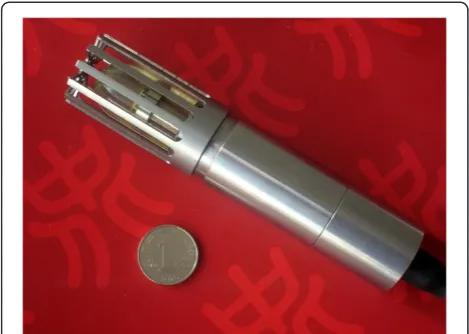
Combining the Micro Electronic Mechanical Systems (MEMS) technology with design of vector hydrophone, it can break the performance limitation of existing hydrophone. A novel biomimetic MEMS vector hydro-phone has been developed by Xue and co-authous (Figure 1), and has been measured for index [9-12].

In this paper, a self-adapting root-MUSIC algorithm and its real-valued formulation for acoustic vector sen-sor array are proposed. Furthermore, the comparison of performance between this algorithm and MUSIC algo-rithm has been made by simulation method. Finally, the engineering practicability has been tested according to the experimental data of MEMS vector hydrophone array in lake trials.

2. Signal model of acoustic vector sensor array Consider N far-field narrowband signals incident on an uniform line array of M acoustic vector sensors along the x-axis in space, from directions θ= [θ1,θ2,⋯,θN]T,

the received signal vector of the array can be expressed as

Zð Þ ¼t Að Þθ Sð Þ þt Nvð Þt ; ð1Þ

where Z(t) is the 3M× 1 snapshot data vector of the array, S(t) is the N ×1 vector of the signal, Nv (t) is the

* Correspondence:[email protected] 1

Key Laboratory of Instrumentation Science & Dynamic Measurement, North University of China, Taiyuan 030051, China

2

Science and Technology on Electronic Test & Measurement Laboratory, North University of China, Taiyuan 030051, China

Full list of author information is available at the end of the article

3M× 1 vector of the Gaussian noise data vector, and the noise and the signal are independent, A(θ) is the steering vector matrix of the acoustic vector sensor array.

Að Þ ¼θ ½að Þθ1 ;að Þθ2 ;⋯;að ÞθN

¼½a1ð Þθ1 ⊗u1;a2ð Þθ2 ⊗u2;⋯;aNð ÞθN ⊗uN; ð2Þ

where akð Þ ¼θk 1;ejβk;ej2βk;⋯;ej Mð 1ÞkT is the acoustic pressure corresponding of the kth signal, β_k¼

2π

λ dsinθk, in which d is the inter-element spacing, and

λ is the wavelength corresponding to the maximum fre-quency of signals. uk= [1, cosθk, sinθk]T is the direction

vector of the kth signal, and the notation ⊗ denotes the Kronecker product.

So the covariance matrix for the array received signal is given by

R¼EZð Þt ZHð Þt

¼AESð Þt SHð Þt AHþENð Þt NHð Þt

¼ARSAHþσ2I; ð3Þ

whereRSis the signal covariance matrix,σ2is the energy

of Gaussian white noise, I is the normalized noise co-variance matrix, and (⋅)H stands for complex conjugate transpose.

From the theory of subspace decomposition, the eigen-decomposition is

R¼USΣSUHS þUNΣNUHN; ð4Þ

whereUSis the signal subspace spanned by eigenvectors

corresponding to major eigenvalues of matrix R, UN is

the noise subspace spanned by eigenvectors correspond-ing to small eigenvalues of matrixR.

In practical calculation, the received data are finite, so the covariance matrixRcan be estimated as

^

R¼1

L

XL

i¼1

Zð Þt ZHð Þt ; ð5Þ

whereLis the number of snapshots.

3. Self-adapting root-MUSIC algorithm for vector sensor array

The basic idea of self-adapting root-MUSIC algorithm is: firstly weight summation for three-way signal of vector sensor, select the self-adaptive lead orientation, then construct polynomial by noise subspace, and finally esti-mate DOA of signals by finding the roots of polynomial.

Selection of lead orientation vector

Weight 1, cosφ, sinφ to the output signal pi(t),vix(t),

viy(t) of ith vector sensor respectively, and make sum

yið Þ ¼t pið Þ þt vixð Þt cosφþviyð Þt sinφ; ð6Þ

then the average power is Pi(φ) = E[|yi(t)|2].

The function of weight corresponds to make electronic rotary for the output of the vector sensor, the direction

φwhich reflects the maximum energy is the signal direc-tion [13].

Pi(φ) is the output of spatial spectrum of ith vector

sensor withφrelevant, reflects the energy distribution in space. It is the equivalent of a spatial filter, and can im-plement the signal and noise separation based on the orientation difference of the signal and interference.

The vector form of (6) for vector sensor array can be written as

Y¼W⋅Z;

whereW= diag[1, cosφ, sinφ,⋯, 1, cosφ, sinφ]. Take

Pð Þ ¼φ 1 M

XM

i¼1

Pið Þφ ; ð7Þ

where P(φ) is spatial spectrum of array. The lead orien-tationφ0can be obtained from the maximum of P(φ) for

φ∈[0, 2π].

The lead orientation vector can be received as

u¼½1;cosφ₀;sinφ₀T; ð8Þ

whereuis also known as self-adaptive lead vector.

Construction of the polynomial

Define the polynomial

f zð Þ ¼zM1FTð1=zÞUNUHNFð Þz ; ð9Þ

where F(z) = [1,z,⋯,zM−1]T⊗u,z= exp(jβ),β= (2π/λ)d

sinθ, and θ is the azimuth angle of the signals to be estimated.

Let

B¼

b11 b12 ⋯ b1M

b21 b22 ⋯ b2M

⋮ ⋮ ⋱ ⋮

bM1 bM2 ⋯ bMM

0 B B @ 1 C C

A¼UNUHN; ð10Þ

where bij (i,j= 1, 2,⋯,M) are 3 × 3 symmetry

sub-matrix. Then

f zð Þ ¼zM1FTð1=zÞBFð Þ ¼z ubM1uH

þzuX 2

i¼1

biþM2;iuTþ⋯þzM1u

XM

i¼1

bi;iuT

þzMuX

M1

i¼1

bi;iþ1uTþ⋯þz2M3u

X2

i¼1

bi;iþM2uT

þz2M2_ub 1MuT¼

XM

k¼1

uXk i¼1

biþMk;iuT

! zk1

þMX 1

k¼1

uMX k

i¼1

bi;iþkuT

!

zMþk1; ð11Þ

So the order of the polynomial f(z)is 2(M−1), it has (M−1) pair roots which every two conjugate with each another. and there areNroots which lie on the unit circle,

zi¼ exp jβi ;i¼1;2;⋯;N:

In practical calculation, considering the error of co-variance matrix, theNroots ^zi nearest to the unit circle can be estimated as the DOAs of the signals.

^

θi¼ arcsin λ

2πd argf g^zi

;i¼1;2;⋯;N: ð12Þ

To sum up, the self-adapting root-MUSIC algorithm can be formulated as the following six-step procedure:

Step 1: ComputeRby (3), and the estimate is given by (5).

Step 2: Obtain UN from the eigendecomposition of R

by (4).

Step 3: Compute the lead vectoruby (8). Step 4: Construct the polynomialf(z) by (11).

Step 5: Find the root of the polynomialf(z), and select the roots ^_zi that are nearest to the unit circle as being the roots corresponding to the DOA estimates.

Step 6: Receive^θito the DOA estimates by (12).

4. RV-Root-MUSIC algorithm

In the above method, the computational complexity will be reduced greatly if making eigendecomposition for a real-valued matrix instead of complex covariance matrix R[14]. The specific process is as follows:

Define

J3M ¼JM⊗I3; ð13Þ

whereJMis theM×Mexchange matrix with ones on its

antidiagonal and zeros elsewhere, and I3is a 3 × 3 iden-tity matrix.

Import the Forward-Backward(FB) smoothing matrix RFBas[15],

RFB¼

1

2 RþJ3MR _J

3M

ð Þ; ð14Þ

where (⋅)*stands for complex conjugate.

The real-valued covariance matrix C can be obtained by

C¼PH_R

FBP; ð15Þ

where P=Q⊗I3 is a sparse matrix with real-valued conversion [14], and matrix Qcan be chosen for arrays with an even and odd number of sensors respectively by (16) and (17).

Q2n¼ 1

ffiffiffi

2

p In jIn Jn jJn

; ð16Þ

Q2nþ1¼

1

ffiffiffi

2

p 0InT p0ffiffiffi_{2 0}jITn

Jn 0 jJn

0 @

1

A_; ð17Þ

where0is then× 1zero vector.

It is proved that C is a real-valued covariance matrix as follows.

Because ofQ*=JQ,JQ*=QandJH=J, then

PH_J

3MRJ3MP¼ðQ⊗I3ÞHðJM⊗I3ÞRðJM⊗I3ÞðQ⊗I3Þ

¼ QH_⊗I

3

JM⊗I3

ð ÞR _J

M⊗I3

ð ÞðQ⊗I3Þ

¼ QH_J M

⊗I3

R _J

MQ

ð Þ⊗I3

½

¼ _ðQ_ÞH_⊗I

3

h i

R_Q⊗I

3

½

¼½ðQ⊗I3ÞHR½Q⊗I3

¼_{ð Þ}P H_RP¼PH_{RP; ð18Þ}

So,

C¼PH_R

FBP¼

1 2 P

H_RPþPH_J

3MRJ3MP

¼RePHRP; ð19Þ

Let the eigendecompositions of the matrix C be defined in a standard way

C¼ESΛSEHS þENΛNEHN; ð20Þ

Similarly to (9), the real-valued root-MUSIC polynomial can be used

f zð Þ ¼zM1FTð1=zÞENEHNFð Þz ; ð21Þ

The computational complexity of self-adapting root-MUSIC algorithm and its real-valued formulation is discussed as follows.

The mainly difference between two methods is that the processing of the covariance matrix. Firstly, the reconstruction of covariance matrix R by (14) and (15) is necessary for RV-Root-MUSIC algorithm, Since the array covariance matrixR is a 3M× 3M complex matrix, the matrixCcan be constructed using 2⋅(3M)3real multiplications and (3M)2(3M−1) real additions by (19).

Secondly, the velocity of convergence for eigendecom-position of the complex matrix Cand the real matrix R is O(n3). simultaneously, the noise subspace of the com-plex matrixRis also complex, and the noise subspace of the real matrixCis also real.

Finally, the polynomial f(z) can be constructed via complex matrixR using 4[(3M)2(3M−N) + (3M)2+ 3M] real multiplications and 3[(3M)2(3M−N−1) + (3M+ 1) (3M−1)] real additions by (9), but the polynomial f(z) can be constructed via real matrix C using [(3M)2 (3M−N) + (3M)2+ 3M] real multiplications and [(3M)2 (3M−N−1) + (3M+ 1)(3M−1)] real additions by (21), so it is possible that the computational complexity for real matrix Ccan be reduced up to 75% real

multiplications and 66.7% real additions compared to the complex matrix R.

From the above analysis, the computational complexity of the RV-Root-MUSIC algorithm is significantly lower than the self-adapting root-MUSIC algorithm thanks to the eigendecomposition of the real-valued matrix C instead of that of the complex matrix R. On the other hand, due to the inherent forward-backward averaging effect by (14), RV-Root-MUSIC algorithm can separate two completely coherent sources and provides improved estimates for correlated signals. This will be validated in the last experiment of lake trials.

5. Simulation experiment

To verify the performance of the proposed self-adapting root-MUSIC algorithm and RV-Root-MUSIC algorithm, simulation experiments are carried out in the following.

The experiment employs the uniform linear array composed of four vector sensors, receives a signal with the frequency being 1kHz and the angle of incidence being 30°, in which inter-element spacing is half wavelength and the adding noise is Gaussian white noise, and assumes the Signal-to-Noise (SNR) being 0dB and the number of snapshots being 200. The DOA estimation using self-adapting root-MUSIC algorithm is shown in Figure 2,

Figure 2DOA estimation of self-adapting root-MUSIC algorithm.

Figure 3The curve between RMSE and SNR of three methods.

where the notation “*” stands for all roots of polynomial,

“o” for the DOA estimation, and “-” for the unit circle. From Figure 2, it can be seen that the DOA of signal can be correctly estimated using self-adapting root-MUSIC algorithm.

In addition, the performance between the proposed self-adapting root-MUSIC algorithm, the RV-Root-MUSIC algorithm and the traditional MUSIC algorithm is compared. In Figure 3, the root mean square error (RMSE) using 500 independent Monte Carlo trials for each SNR is shown when SNR changes from −20dB to 20dB. The proposed self-adapting root-MUSIC algorithm and the RV-Root-MUSIC algorithm have identical performance, and they have better performance for low SNRs and almost the same estimation perform-ance for high SNRs with MUSIC algorithm.

Finally, In the above simulation conditions, the statis-tics for computing time of two algorithms has been made, and it is shown that the integrated computing time of the RV-Root-MUSIC algorithm is average less

about 23% than the self-adapting root-MUSIC algorithm by comparing two methods. Certainly, the computing time of the RV-Root-MUSIC algorithm can be reduced more with the increase of the number of array elements.

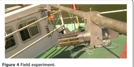
6. Lake trials

The test experiment has been made in the Fenhe lake (Figure 4). The line array has been composed of two MEMS vector hydrophone with inter-element spacing being 0.5 m, and it has been fixed underwater 10 m at the side of the ship. The array’s compass could take real-time measurement for its pose to keep the array’s horizontality. Three experiments have been made respectively.

Experiment 1

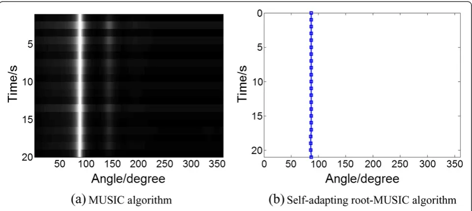
The acoustic emission transducer has been placed in the direction with 90° of the array, launched 331Hz, 800Hz, 1kHz, 1.5kHz,3kHz continuous single-frequency signal re-spectively, the DOA has been estimated for receiving data, once per second. Table 1 is the average result of DOA esti-mation in different frequency signal using MUSIC algo-rithm and self-adapting root-MUSIC algoalgo-rithm, Figure 5 is the time-bearing display of a single-frequency signal with 1.5kHz using two methods. The result shows the better performance of two methods.

Experiment 2

The experiment used a motor boat for moving target, which run from about 10° to about 160° position, tested track time is about 160s. Broadband noise which motor boat radiate has been narrowband filtered as 800Hz

Table 1 The DOA estimation result of different frequency signal using two methods

Signal frequency

Average of DOA estimation of MUSIC

algorithm(°)

Average of DOA estimation of self-adapting root-MUSIC

algorithm(°)

331Hz 90.2768 90.0377 800Hz 89.7857 89.8085 1kHz 89.8571 89.8598 1.5kHz 89.8636 89.4449 3kHz 89.6324 89.7719

for the center frequency, once per second. Figure 6 shows the time-bearing display of target ship using MUSIC algorithm, conventional beam-forming method (which is also known as Bartlett beam-forming for acous-tic vector sensor array) and self-adapting root-MUSIC al-gorithm respectively, the results are basically consistent with the actual trajectory of motor boat.

Experiment 3

The experiment used motor boat and emission trans-ducer for two acoustic sources. The acoustic emission transducer has been placed in the direction with 180° of the array, launched 800Hz continuous single-frequency signal, simultaneously, the motor boat run from about 10° to about 180° position, tested track time is about 108s. Broadband noise which motor boat radiate has

been narrowband filtered as 800Hz for the center fre-quency, once per second.

Here, these two sources can be seen the coherent signals. First the real-valued covariance matrix C is homologous used to replace the complex matrixRin MUSIC algorithm and conventional beam-forming method, and then the time-bearing display of two sources using three methods respectively can be seen in Figure 7. The MUSIC algo-rithm can be more clearly distinguish between these two sources at the outset, but there will be some ambiguity when two sources approached (Figure 7(a)), and conven-tional beam-forming method is completely unable to dis-tinguish (Figure 7(b)), but the RV-Root-MUSIC algorithm can clearly distinguish (Figure 7(c)), the results are basically consistent with the actual trajectory of motor boat and emission transducer.

7. Conclusions

The results of simulation experiment show the higher DOA estimation accuracy and lower RMSE of the new self-adapting root-MUSIC algorithm and the RV-Root-MUSIC algorithm than the traditional RV-Root-MUSIC algo-rithm, and the results in lake trails show the engineering practicability of two new algorithms, it can be verified that the performance of RV-Root-MUSIC algorithm distinguishing the coherent signals.

Competing interests

The authors declare that they have no competing interests.

Acknowledgements

This work is supported by the National Nature Science Foundation of China (Grant No. 61127008) and International Science & Technology Cooperation Program of China (Grant No.2010DFB10480).

Author details

1_{Key Laboratory of Instrumentation Science & Dynamic Measurement, North}

University of China, Taiyuan 030051, China.2_{Science and Technology on}

Electronic Test & Measurement Laboratory, North University of China, Taiyuan 030051, China.3_{School of Science, North University of China, Taiyuan 030051,}

China.

Received: 17 February 2012 Accepted: 10 October 2012 Published: 25 October 2012

References

1. C.B. Lesie, J.M. Kendall, J.L. Jones, Hydrophone for measuring particle velocity. J Acoust Soc Am28, 711_–715 (1956)

2. M.J. Berliner, J.F. Lindberg,Acoustic Particle Velocity Sensors: Design, Performance and Applications, American Institute of Physics(Woodbury, New York, 1996)

3. G.Q. Sun, Q.H. Li, Progress of study on acoustic vector sensor. ACTA ACUSTICA29(6), 481–490 (2004). in Chinese

4. A. Nehorai, E. Paldi, Acoustic vector sensor array processing IEEE Trans. Signal Process42(9), 2481–2491 (1994)

5. P. Stoica, A. Nehorai, MUSIC, maximum likelihood and Cramer-Rao bound, IEEE Trans. Acoust. Speech, Signal Process37(5), 2296–2299 (1989) 6. M. Hawkes, A. Nehorai, Acoustic Vector-Sensor Beamforming and Capon

Direction Estimation. IEEE Trans. Signal Process.46, 2291–2304 (1998) 7. M.D. Zoltowski, G.M. Kautz, S.D. Silverstein, Beamspace root-MUSIC. IEEE

Trans Signal Process41(1), 344–364 (1993)

8. B.D. Rao, K.V.S. Hari, Performance analysis of root-MUSIC. IEEE Trans. Acoust., Speech, Signal Process37(12), 1939–1949 (1989)

9. C.Y. Xue, Z.M. Tong, B.Z. Zhang, A novel vector hydrophone based on the piezoresistive effect of resonant tunneling diode. IEEE Sensors Journal8(4), 401–402 (2008)

10. C.Y. Xue, S. Chen, W.D. Zhang, Design, fabrication and preliminary characterization of a novel MEMS bionic vector hydrophone. Microelectronics Journal38, 1021–1026 (2007)

11. T.D. Wen, L.P. Xu, J.J. Xiong, W.D. Zhang, The meso-piezo-resistive effects in MEMS/NEMS. Solid State Phenomena, 121–123 (2007). 619–622

12. W.D. Zhang, C.Y. Xue, J.J. Xiong, Piezoresistive effects of resonant tunneling structure for application in micro-sensors. Indian Journal of Pure & Applied Physics45, 294–298 (2007)

13. N. Jiang, J.G. Huang, S. Li, DOA estimation algortithm based on single acoustic vector sensor. Chinese Journal of Scientific Instrument25(4), 87–90 (2004). in Chinese

14. M. Pesavento, A.B. Gershman, M. Haardt, Unitary Root-MUSIC with a Real-Valued Eigendecomposition: A Theoretical and Experimental Performance Study. IEEE Trans. Signal Process48(5), 1306–1314 (2000) 15. D.A. Linebarger, R.D. DeGroat, E.M. Dowling, Efficient Direction-Finding Methods Employing Forward/Backward Averaging. IEEE Trans. Signal Process42(8), 2136–2145 (1994)

doi:10.1186/1687-6180-2012-228

Cite this article as:Wanget al.:Self-adapting root-MUSIC algorithm and

its real-valued formulation for acoustic vector sensor array.EURASIP Journal on Advances in Signal Processing20122012:228.

Submit your manuscript to a

journal and benefi t from:

7Convenient online submission

7Rigorous peer review

7Immediate publication on acceptance

7Open access: articles freely available online

7High visibility within the fi eld

7Retaining the copyright to your article