University of Windsor University of Windsor
Scholarship at UWindsor
Scholarship at UWindsor
Electronic Theses and Dissertations Theses, Dissertations, and Major Papers
2011
Generalized Estimating Equations and Gaussian Estimation in
Generalized Estimating Equations and Gaussian Estimation in
Longitudinal Data Analysis
Longitudinal Data Analysis
Xuemao ZhangUniversity of Windsor
Follow this and additional works at: https://scholar.uwindsor.ca/etd
Recommended Citation Recommended Citation
Zhang, Xuemao, "Generalized Estimating Equations and Gaussian Estimation in Longitudinal Data Analysis" (2011). Electronic Theses and Dissertations. 5400.
https://scholar.uwindsor.ca/etd/5400
This online database contains the full-text of PhD dissertations and Masters’ theses of University of Windsor students from 1954 forward. These documents are made available for personal study and research purposes only, in accordance with the Canadian Copyright Act and the Creative Commons license—CC BY-NC-ND (Attribution, Non-Commercial, No Derivative Works). Under this license, works must always be attributed to the copyright holder (original author), cannot be used for any commercial purposes, and may not be altered. Any other use would require the permission of the copyright holder. Students may inquire about withdrawing their dissertation and/or thesis from this database. For additional inquiries, please contact the repository administrator via email
Generalized Estimating Equations
and Gaussian Estimation
in Longitudinal Data Analysis
by
Xuemao Zhang
A Dissertation
Submitted to the Faculty of Graduate Studies
through the Department of Mathematics and Statistics
in Partial Fulfillment of the Requirements for
the Degree of Doctor of Philosophy at the
University of Windsor
Windsor, Ontario, Canada
2011
GEE and Gaussian Estimation in
Longitudinal Data Analysis
by
Xuemao Zhang
APPROVED BY:
—————————————————————–
Dr. P. Song, External Examiner
University of Michigan
—————————————————————–
Dr. Y. Aneja
Odette School of Business
—————————————————————–
Dr. A. A. Hussein
Department of Mathematics and Statistics
—————————————————————–
Dr. M. Hlynka
Department of Mathematics and Statistics
—————————————————————–
Dr. S. R. Paul, Advisor
Department of Mathematics and Statistics
—————————————————————–
Dr. K. Taylor, Chair of Defense
Department of Chemistry and Biochemistry
Author’s Declaration of Originality
I hereby certify that I am the sole author of this thesis and that no part of this
thesis has been published or submitted for publication. I certify that, to the best of
my knowledge, my thesis does not infringe upon anyone’s copyright nor violate any
proprietary rights and that any ideas, techniques, quotations, or any other material
from the work of other people included in my thesis, published or otherwise, are fully
acknowledged in accordance with the standard referencing practices. Furthermore,
to the extent that I have included copyrighted material that surpasses the bounds of
fair dealing within the meaning of the Canada Copyright Act, I certify that I have
obtained a written permission from the copyright owner(s) to include such material(s)
in my thesis and have included copies of such copyright clearances to my appendix. I
declare that this is a true copy of my thesis, including any final revisions, as approved
by my thesis committee and the Graduate Studies office, and that this thesis has not
Abstract
In this dissertation, we first develop a Gaussian estimation procedure for the
es-timation of regression parameters in correlated (longitudinal) binary response data
using working correlation matrix and compare this method with the GEE (generalized
estimating equations) method and the weighted GEE method. A Newton-Raphson
algorithm is derived for estimating the regression parameters from the Gaussian
like-lihood estimating equations for known correlation parameters. The correlation
pa-rameters of the working correlation matrix are estimated by the method of moments.
Consistency properties of the estimators are discussed. A simulation comparison of
efficiency of the Gaussian estimates and the GEE estimates of the regression
param-eters shows that the Gaussian estimates using the unstructured correlation matrix
of the responses for a subject are, in general, more efficient than those by the other
methods compared. The next best are the Gaussian estimates using the general
autocorrelation structure. Two data sets are analyzed and a discussion is given.
The main advantage of GEE is its asymptotic unbiased estimation of the marginal
regression coefficients even if the correlation structure is misspecified. However, the
technique requires that the sample size should be large. In this dissertation, two
bias corrected GEE estimators of the regression parameters in longitudinal data are
proposed when the sample size is small. Simulations show that the proposed methods
do well in reducing bias and have, in general, higher efficiency than the GEE estimates.
Two examples are analyzed and a discussion is given.
The current GEE method focuses on the modeling of the working correlation
if the variance function is misspecified, the correct choice of the correlation structure
may not necessarily improve estimation efficiency for the regression parameters. In
this dissertation, we propose a GEE approach to estimate the variance parameters
when the form of the variance function is known. This estimation approach borrows
the idea of Davidian and Carroll (1987) by solving a non-linear regression problem
where residuals are regarded as the responses and the variance function is regarded
as the regression function. Simulations show that the proposed method performs as
Dedication
This thesis is dedicated to my wife, Yuxia Niu. I thank her for her love and
support throughout the years. It is also dedicated to my parents who have been a
Acknowledgements
I would like to express my profound gratitude to my supervisor Dr. Paul. He
never hesitated to provide me assistance when I need help throughout my study.
The doctoral program under his supervision has prepared me well for my future
professional career. This dissertation could not have been accomplished without his
insights into all the statistical subjects. He also has made numerous very useful
suggestions to the thesis composition including wording and grammar. Moreover, I
am very grateful to Dr. Paul for the Research Assistantship he has provided to me.
I would like to thank Dr. Hlynka and Dr. Hussein as the department readers.
Their remarks have made the thesis more rigorous and readable. I am also grateful
to Dr. Aneja of the Department of Management Science, Odette School of Business,
University of Windsor and Dr. Song of University of Michigan for their valuable
comments and suggestions.
I would like to thank the University of Windsor for providing me a Graduate
Assistantship, and the Ontario Ministry of Training, Colleges and Universities for
providing me an Ontario Graduate Scholarship during my graduate study. These
financial supports have enabled me to finish the doctoral program more easily.
Last but not least, I wish to thank my wife and my parents for their constant
love, encouragement and support. They have always been eager to help me in any
Contents
Author’s Declaration of Originality iii
Abstract v
Dedication vi
Acknowledgements vii
List of Tables xi
List of Figures xiii
Chapter 1. Introduction 1
Chapter 2. Literature Review 8
2.1. Definitions and rules in matrix calculus 8
2.2. Generalized linear models 10
2.3. Quasi-likelihood 11
2.4. Generalized estimating equations 12
2.5. Gaussian copula regression models 18
Chapter 3. Gaussian Estimation for Longitudinal Binary Data 20
3.1. Introduction 20
3.2.1. Estimation of the regression parameters 23
3.2.2. Consistency of the estimates of the parameters 26
3.2.3. Variance of ˆβ 27
3.3. Simulations 28
3.4. Examples 33
3.5. Discussion 37
Chapter 4. Bias Correction for GEE Estimation 40
4.1. Introduction 40
4.2. Estimates of the Regression Parameters Based on Bias-correction and
Bias-reduction for Longitudinal Data 41
4.3. Application to binary and count data 45
4.3.1. Binary data 45
4.3.2. Count data 46
4.4. Simulations 46
4.5. Examples 56
4.6. Discussion 57
Chapter 5. Effects of Variance Function on Estimation Efficiency 59
5.1. Introduction 59
5.2. Modified pseudo-likelihood approach (Wang and Zhao, 2007) 60
5.3. Estimating parameters of the variance function using generalized
estimating equations 62
Chapter 6. Conclusions and Future Research 70
6.1. Marginal regression analysis of longitudinal data with time-dependent
covariates 71
Appendix A 75
Appendix B 76
Appendix C 77
Appendix D 78
Appendix E 81
Appendix F 83
Bibliography 85
List of Tables
3.1N× average estimated variance for ˆβ0 and ˆβ1 by Gaussian estimation procedure
using the four working correlation structures: data generated from MP model with
latent (i) exchangeable R(0.5); (ii) AR(1) R(0.5); (iii) general autocorrelation
matrix A and (iv) unstructured covariance matrix U; xij ∼ uniform(-1,1); p=2,
β0=0.0, β1 =0.5; observation times d=5; based on 500 iterations. 30
3.2N× average estimated variance for ˆβ0 and ˆβ1 by ML, Gaussian-Autocorr,
Gaussian-Unstr and GEE methods: data generated from MP model with latent (i)
exchangeableR(0.5); (ii) AR(1)R(0.5); (iii) general autocorrelation matrix Aand
(iv) unstructured covariance matrixU;xij ∼uniform(-1,1);p=2, β0=0.0, β1=0.5;
observation times d=5; based on 500 iterations. 32
3.3Results of the regression analysis of the wheezing status data; estimates ofβ0,β1,
β2 and β3 of the model (3.4.1) with standard errors in parenthesis using maximum
likelihood method based on the MP model, four Gaussian estimation methods and
six GEE procedures; with probit link. 34
3.4Results of the regression analysis of the complete Mluscatinie Study data; estimates
of β0,β1,β2 and β3 of the model (3.4.2) with standard errors in parenthesis using
four Gaussian estimation methods and six GEE procedures; with probit link. 36
List of Figures
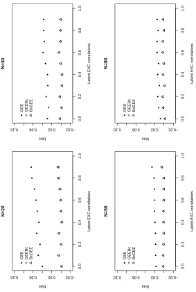
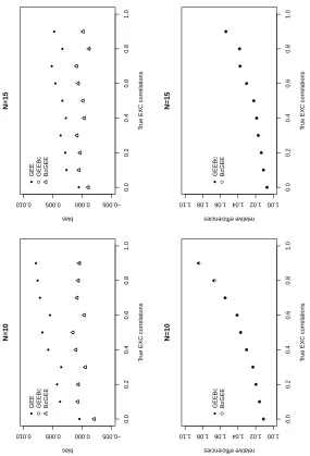
4.1 Biases of ˆβ1, ˜β1 and β1∗ with latent exchangeable correlations in MP model. 49
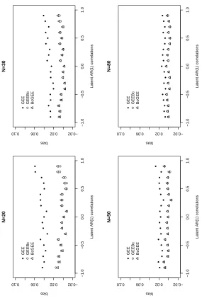
4.2 Biases of ˆβ1, ˜β1 and β1∗ with latent AR(1) correlations in MP model. 50
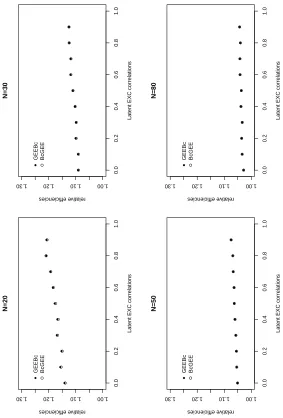
4.3 Relative efficiency of ˜β1 and β1∗ with latent exchangeable correlations in MP
model. 52
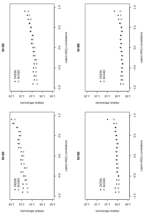
4.4 Relative efficiency of ˜β1 and β1∗ with latent AR(1) correlations in MP model. 53
4.5 Biases and relative efficiencies of ˆβ1, ˜β1 and β1∗ for exchangeable Poisson
data. 55
5.1Comparison of MSE of ˆβ1 for longitudinal normal data by fixingγ in the power function
at 0 (○), 1.5(◇), 2.5(●), 3.5(▲) or estimating γ by the proposed method (△) and the
pseudolikelihood method (◆). Data are generated from either AR(1) or EXC correlation
structures. The working correlation structure is either AR(1) or EXC. The true values are
β0=0, β1=1 andγ=1.5. 66
5.2Comparison of MSE of ˆβ1 for longitudinal normal data generated using the power variance
functionγ1µγ2. In estimation the power variance function is used where the parameters
are estimated by the pseudolikelihood method (▲) and the proposed method (◇) or the
Bartlett function is used where the parameters are estimated by the pseudolikelihood
correlation structures. The working correlation structure is either AR(1) or EXC. The true
values areβ0=0, β1=1 and the parameters in the power functionγ1=1 andγ2=1.5. 68
5.3Comparison of MSE of ˆβ1 for longitudinal normal data generated using the Bartlett
variance function γ1µγ2. In estimation the power variance function is used where
the parameters are estimated by the pseudolikelihood method (▲) and the proposed
method (◇) or the Bartlett function is used where the parameters are estimated by the
pseudolikelihood method (●) and the proposed method (△). Data are generated from
either AR(1) or EXC correlation structures. The working correlation structure is either
AR(1) or EXC. The true values areβ0=0, β1=1 and the parameters in the power function
CHAPTER 1
Introduction
Longitudinal data arise in many fields such as biomedical and social sciences. Longitudinal data are characterized by repeated measurements taken on each of a number of subjects over time. In these studies it is reasonable to assume that the subjects are independent, but the repeated measurements taken on each subject may not be uncorrelated. The purpose of longitudinal data analysis is to model the rela-tionship of the repeated measurements of each subject to the associated covariates. As an example consider the data from the Six Cities study, a longitudinal study of the health effects of air pollution that was analyzed by Fitzmaurice and Laird (1993). The data set contains complete records on 537 children from Steubenville, Ohio, each of whom was examined annually at ages 7 through 10. The repeated binary response is the wheezing status (1=yes, 0=no) of a child at each occasion. The purpose of the study is to model the probability of the wheezing status as a function of the child’s age, his/her mother’s maternal smoking habit (a binary variable MS with 1 if the mother smoked regularly and 0 otherwise) and their interactions.
to characterize the marginal expected value of a subject’s response as a function of the subject’s covariates. Diggle, Liang and Zeger (1994) discussed these models in detail. The study of the marginal model of longitudinal data analysis is our focus in this thesis.
The complication of longitudinal data analysis is partly due to the lack of a rich class of models such as the multivariate normal for the joint distribution of the re-sponses of a subject. Therefore, a robust method that avoids full distributional as-sumptions of the likelihood approach is required. One such method is the generalized estimating equations (GEE) approach proposed by Liang and Zeger (1986) and Zeger and Liang (1986). The GEE method is developed from the theory of generalized lin-ear models (GLM) by Nelder and Wedderburn (1972) and optimal inference functions established by Godambe (1960).
correlation between the repeated measurements of a subject. The GEE estimator for the regression parameter β is consistent even if the working correlation structure is misspecified. However, correct specification of the correlation structure can improve the estimation efficiency of the regression parameter (Wang and Carey, 2003).
Gaussian estimation introduced by Whittle (1961) is another estimation technique with no distributional assumptions. It uses the normal log-likelihood as the estima-tion funcestima-tion without assuming that the data are normally distributed. The Gaussian estimation procedure has been shown to have good properties in a number of applica-tions. For example, Crowder (1985) showed by simulation that a Gaussian estimate of the correlation parameter of equi-correlated clustered binary data has high efficiency. Paul and Islam (1998), again, by simulation, showed that a Gaussian estimator of the overdispersion parameter in clustered binomial data has best efficiency in com-parison to likelihood, quasi-likelihood and extended quasi-likelihood estimates. Wang and Zhao (2007) used Gaussian estimation for the analysis of longitudinal data when the covariance function is modelled by additional variance parameters to the mean parameters.
For the working covariance matrix in GEE, the current method focuses only on the modeling of the working correlation R(ρ) and the variance function v is treated as known which is of the form in GLM, a function of the marginal meanµ. However, in practice the distribution of the data may not be from a GLM and we tend to choose a wrong variance function. Wang and Lin (2005) investigated the impacts of misspecifying the variance function on estimators of the regression parameters. They show that if the variance function is misspecified, the scorrect choice of the correlation structure may not necessarily improve estimation efficiency. This can be understood from the logic that modeling of the correlation structure is based on the correct modeling of the variance function. The best choice of the working correlation may no longer be the true one for estimating β if the specified variance function is far from the true one (Wang and Zhao, 2007). Therefore, the variance function plays a more important role than the correlation structure.
In this dissertation, we deal with three problems. We first explore Gaussian es-timation for longitudinal data to improve eses-timation efficiency. Second, we propose two bias correction procedures to reduce the biases of GEE estimates of regression parameters when the sample size is small. Last, we investigate how the variance functions affect the estimation efficiency and propose a GEE approach to estimate the additional variance parameters in the variance function to improve estimation ef-ficiency. This estimation approach borrows an idea of Davidian and Carroll (1987) by solving a non-linear regression problem where residuals are regarded as the responses and the variance function is regarded as the regression function.
In Chapter 3, we study Gaussian estimation for longitudinal binary data. The purpose of this chapter is to develop and investigate the Gaussian estimation proce-dure for the estimation of regression parameters in longitudinal binary response data and compare this method with the GEE and related methods. As in the GEE we use a working correlation matrix for the responses of each individual. Consistency of the estimates of the regression parameters is ensured by carefully choosing a robust working correlation structure: general autocorrelation or unstructured. Efficiencies of the estimates are then compared with the GEE method and the weighted GEE approach by Chaganty and Joe (2004).
In Chapter 4, we study bias-correction in GEE estimation. By treating the GEE function as a likelihood score function, we apply the bias correction technique of Cordeiro and Klein (1994) and Firth (1993). The former method is corrective. That is, the GEE estimator is first calculated then corrected. The latter method is preventive in which a bias term is introduced into the GEE function.
In Chapter 5, we focus on the study of effects of variance function on the estimation efficiency of the regression parameters. The variance parameters in the variance function of known form are estimated using a GEE approach by solving a non-linear regression problem by regarding the residuals as responses and the variance function as regression function. This idea of the estimation method is borrowed from Davidian and Carroll (1987) in the setting of heteroscedastic regression models. Our proposed method is then compared with the pseudolikelihood approach by Wang and Zhao (2007).
CHAPTER 2
Literature Review
2.1. Definitions and rules in matrix calculus
In this section, we review the definition of the derivative of a function and the chain rule, product rule and the Kronecker product rule in matrix calculus (Magnus and Neudecker, 1988).
The vec operator and Kronecker products are used frequently in matrix calculus. The vec operator vectorizes a matrix by stacking the columns of the matrix one under the other. Let A be an m×n matrix and B a p×q matrix. The Kronecker product
A⊗B of A and B which is mp×nq dimensional is defined by ⎛
⎜⎜ ⎜⎜ ⎜⎜ ⎝
a11B ⋯ a1nB
⋮ ⋮
am1B ⋯ amnB
⎞ ⎟⎟ ⎟⎟ ⎟⎟ ⎠
.
Letf be a scalar function of ann×1 vector x. The derivative of f is defined as
Df(x) = (D1f(x), . . . , Dnf(x)) =
∂f(x)
∂x ,
where Djf is the derivative of f with respect to the jth variable, holding the other
variables fixed. If f is anm×1 vector function of x, then the derivative (orJacobian
matrix) of f is the m×n matrix
Df(x) =∂f(x)
∂x with [Df]ij =
∂fi(x)
∂xj
.
Definition 2.1.1. Let F be a differentiable m×p real matrix function of an n×q
matrix of real variables X. The Jacobian matrix of F at X is the mp×nq matrix
DF(X) =∂vecF(X)
∂(vecX) .
A general product rule is defined as follows. Suppose that f ∶ Rn →
Rm×p and
g∶Rn→
Rp×q, so f(x)g(x) ∶Rn→Rm×q. Then
Df(x)g(x) = (g(x)T ⊗Im)Df(x) + (Iq⊗f(x))Dg(x). (2.1.1)
Furthermore, thechain rule involves matrix multiplication, which requires conforma-bility. Given two functions f ∶ Rn →
Rm and g ∶ Rp → Rm, the derivative of the
composite function is
D[f(g(x))] =f′(g(x))g′(x).
Definition 2.1.2. Let A be an m×n matrix. The vectors vec A and vec AT
clearly contain the same mn components, but in a different order. Hence there exists
a unique mn×mn permutation matrix which transforms vec A into vec AT. This
matrix is called the commutation matrix and is denoted by Kmn. If m =n, Knn is
often written as Kn.
Theorem 2.1.1. Let U ∶ S → Rn×q and V ∶ S → Rp×r be two matrix functions
defined and differentiable on an open set S in Rm×s. Then the Kronecker product
U⊗V is differentiable on S and
2.2. Generalized linear models
The generalized linear model (GLM) developed by Nelder and Wedderburn (1972) is a generalization of normal linear models. It requires that the response variables be from an exponential family and the expected responses be a function of the linear predictors.
For the scalar observationz, suppose the probability density function is given by
fZ(z;θ, φ) =exp{[zθ−b(θ)]/a(φ) +c(z, φ)} (2.2.1)
for some functions a(⋅), b(⋅) and c(⋅). This is called an exponential family with canonical parameterθ if φ is known. It can be seen that E(Z) =b′(θ). Moreover, the variance of Z is related to its expected value by Var(Z) =b′′(θ)a(φ), where b′′(θ) is called the variance function and φ is called the dispersion parameter.
Let Y and µ be n×1 dimensional vectors. The classical linear model can be rearranged to the following tripartite form (see McCullagh and Nelder, 1983):
1. The random component: Y has independent Normal distribution with con-stant variance σ2 and E(Y) =µ.
2. The systematic component: covariates in the form of an n×pdesign matrix
X= (xT
1, xT2, . . . , xTn)T produce a linear predictor η given by
η=Xβ,
whereβ is a p×1 regression parameter vector.
3. The link between the random and systematic components is given by
µ=η.
includes the normal distribution as a special case. Secondly, the link between the random and systematic components is given by η =g(µ), where g is called the link function which is monotone and differentiable.
2.3. Quasi-likelihood
The quasi-likelihood method proposed by Wedderburn (1974) does not depend on the specification of a full distribution, such as a density function from an exponential family. Instead it just requires the structure of the mean and variance, that is, the first two moments. Moreover, the variance generally is a function of the expected value.
Let y1, . . . , yn be independent responses with means E(yi) = µi and variance
Var(yi) =φv(µi), whereµiis a function of unknown regression parametersβ1, β2, . . . , βp,
v(⋅) is a known variance function andφ is a scalar or dispersion parameter. Then the quasi-likelihood of a single observation yi is given by
Q(µi;yi) = ∫ µi
yi
yi−t
φv(t) dt. (2.3.1)
And the quasi-likelihood for the complete data is given by the sum of the individual contributions
Q(µ;y) =
n
∑
i=1
Q(µi;yi).
The estimates of the regression parameters are obtained by solving a set of score-like equations
Sk(β) =
n
∑
i=1
∂µi
∂βk(
v(µi))−1(yi−µi) =0, k=1, . . . , p.
Lety= (y1, . . . , yn)T andµ= (µ1, . . . , µn)T. Then, in matrix notation, these equations
can be written as
S(β) = (∂µ/∂β)TV−1(
where V =diag{v(µi)}.
For simple models, such as Normal distribution and Poisson distribution, the log likelihood score and the quasi-likelihood function are identical.
2.4. Generalized estimating equations
Generalized estimating equations (GEE) (Liang and Zeger 1986, Zeger and Liang 1986) generalize the quasi-likelihood method to analyze longitudinal/clustered data. In a marginal model, the analyst is interested in modeling the marginal expectation as a function of explanatory variables. The GEEs are used to characterize the marginal expectation of a set of outcomes as a function of a set of covariates.
We illustrate the longitudinal data framework as follows. The clustered data can be described in a similar way. Let yi = (yi1, . . . , yini)
′
be the response vector for the ith subject, i = 1, . . . , N. Assume the N subjects are independent while the repeated measurements taken on each subject are correlated. Associated with each measurement yij is a vector of covariates xij = (xij1, . . . , xijp)
′
, j =1, . . . , ni, i =
1, . . . , N. Let Xi = (xi1, . . . , xini)
′
be the ni ×p design matrix for the ith subject.
Defineµi be the expectation of yi and suppose that
µi=h(Xiβ),
where β is a p×1 vector of regression parameters of interest and the inverse of h is referred as the link function. Also assume that the variance of yij is expressed as a
known monotone function, v, of µij,
Var(yij) =φv(µij), j =1, . . . , ni,
GEE method uses a common working correlation matrix for the longitudinal re-sponses for each subject. The word “working” means that the correlation structure may not be correctly specified. LetR(ρ)be a working correlation matrix completely specified by the parameter vector ρ of length q. Then φWi =φA
1/2
i R(ρ)A 1/2
i is the
corresponding working covariance matrix, where Ai =diag{v(µij)} is a diagonal
ma-trix, i = 1, . . . , N. For given consistent estimates of φ and ρ, the estimate ˆβ is the solution of the GEE equations
N
∑
i=1
DTi W−1
i (yi−µi) =0, (2.4.1)
where Di = ∂µ∂βi. It can be seen that if R(ρ) is an identity matrix, then the GEE
equations are quasi-likelihood estimating equations.
The estimator ˆβ of β obtained by solving GEE equation (2.4.1) is consistent even if the correlation structure is misspecified. However, the misspecification of the correlation structure may result in inefficient estimates of the regression parameters (for more details, see Wang and Carey, 2003).
Given consistent estimates ˆρ and ˆφ of the correlation and dispersion parame-ters, under mild regularity conditions (the parameter space is an open set; the GEE function ∑Ni=1DT
i W
−1
i (yi −µi) is continuously differentiable; ∣∂ρˆ(β, φ)/∂φ∣ ≤ Op(1)
), N1/2(βˆ−β) is asymptotically multivariate normal with mean zero and sandwich
covariance matrix
lim
N→∞
N(
N
∑
i=1
DTi W−1
i Di)
−1
[∑N
i=1
DiTW−1
i Cov(Yi)Wi−1Di] ( N
∑
i=1
DiTW−1
i Di)
−1
.
This covariance matrix is estimated by replacing ˆβ byβand Cov(Yi)by its estimated
covariance matrix (yi−µˆi)T(yi−µˆi). The resulting estimated asymptotic covariance
Instead of using the moment estimates ofφ andρ in generalized estimating equa-tions, when analyzing correlated binary reponses, Prentice (1988) simultaneously modeled the mean and correlation profiles. In the estimation, a second set of GEEs to estimate the correlation parameters is added. The moment estimating equations for ρ is given by
u(ρ) =
N
∑
i=1
AiTHi−1[πi−νi(β, ρ)] =0, (2.4.2)
whereπi= {πi12, πi13,⋯, πi23,⋯}, νi= {νi12, νi13,⋯, νi23,⋯}, πist=yisyit/(pis(1−pis)pit(1−
pit))1/2, νist = E(πist∣xi) for s < t, Ai = ∂νi/∂ρ and Hi =diag(Var(πi)). This simple
estimating equation approach for means and covariances applies similarly to other types of response variables than binary. Prentice (1988) also established asymptotic normality for the joint distribution of his estimates ofβ and ρ.
Lipsitz, Laird and Harrington (1991) modified the estimating equations of Pren-tice and modeled the association between binary responses based on odds ratios. This approach is useful if the odds ratio are of interest themselves, and not confined between (−1,1).
Prentice and Zhao (1991), extending the idea of Prentice (1988), introduced esti-mating equations (GEE2) in an ad hoc fashion for means and covariances. The GEE2 can be written as
N−1/2
N
∑
i=1
DTi V−1
i fi=0, (2.4.3)
whereDi=
⎛ ⎜⎜ ⎝
∂Tµ
i/∂β 0
∂Tσ
i/∂β ∂Tσi/∂ρ
⎞ ⎟⎟ ⎠
,Vi=
⎛ ⎜⎜ ⎝
Var(yi) Cov(yi, si)
Cov(si, yi) Var(si)
⎞ ⎟⎟ ⎠
,fi =
⎛ ⎜⎜ ⎝
yi−µi
si−σi
⎞ ⎟⎟ ⎠ ,
sT
i = (si11, si12,⋯, sidd) with sikl=sikl(β) = (yik−µik)(yil−µil) and σTi = (σi11, σi12,⋯,
σi22,⋯, σidd). Compared to GEE2, GEE1 (the GEE by Liang and Zeger, 1986) can
should be applied if both the mean and covariance parameters are of interest. How-ever, GEE2 is not robust to misspecification of correlation structure. Another problem for GEE2 is that it can become computationally infeasible as the observation times (or cluster size) ni gets large since there are (n2i) estimating equations for the
corre-lation parameters (Carey, Zeger and Diggle, 1993). Therefore, GEE1 should be used when the correlation parameter ρ is considered as a nuisance parameter.
When the working correlation structure is misspecified, one pitfall of the GEE approach is that in some cases ˆρdoes not exist or does not converge which can lead to a breakdown of the asymptotic properties of the regression parameters (Crowder 1995). Crowder (1995) suggested two approaches to avoid the problem. One suggestion is to use only estimating equations which have a guaranteed solution. Another suggestion is to minimize some objective function with respect to ρ.
Adopting the idea of Crowder (1995), Chaganty (1997) presented a new method called quasi-least square (QLS) for estimating the correlation parameters. By the principle of generalized least squares, which requires minimizing the quadratic form
Qφ(β, ρ) =
1
φ
N
∑
i=1
(yi−µi(β))TWi−1(yi−µi(β))
=1
φ
N
∑
i=1
(yi−µi(β))TA
−1/2
i (β)R
−1(
ρ)A−1/2
i (β)(yi−µi(β)),
(2.4.4)
estimating equations for ρ are obtained by taking the partial derivative of Qφ(β, ρ)
with respect to ρand equating it to zero. The resulting estimating equations are
N
∑
i=1
ZT
i
∂R−1(ρ)
∂ρj
Zi=0, 1≤j≤q, (2.4.5)
where Zi=A
−1/2
i (β)(yi−µi(β)),1≤i≤N. And the set of estimating equations for β
The QLS estimates of the regression parametersβ and the dispersion parameterφ
are consistent even if the working correlation structure is misspecified. The estimates of the correlation parameters, however, are asymptotically biased. Chaganty and Shults (1999) proposed a modified (C-QLS) estimate of the correlation parameter to eliminate the asymptotic bias for the following working correlation structures: the unstructured matrix, the exchangeable, tridiagonal, and autoregressive structures.
Another method to bypass the pitfall is to use quadratic inference functions (QIF) developed by Qu, Lindsay and Li (2000). This method is based on the fact that the inverse of the working correlation matrix can be expressed by the linear combination of known basis matrices M1,⋯, Mm. That is,
R−1(
ρ) =
m
∑
l=1
alMl, (2.4.6)
where a1,⋯, am are unknown constants. Plugging this expression into the GEE
(2.4.1), we have
N
∑
i=1
∂µT
i
∂β A
−12
i (a1M1+. . .+amMm)A
−12
i (yi−µi) =0.
Define the extended score gN as
gN(β) =
1
N
N
∑
i=1
gi(β) =
1
N
N
∑
i=1
⎛ ⎜⎜ ⎜⎜ ⎜⎜ ⎝ ˙ µT i A −1 2
i M1A
−1 2
i (yi−µi)
⋮ ˙ µT i A −1 2
i MmA
−1 2
i (yi−µi)
⎞ ⎟⎟ ⎟⎟ ⎟⎟ ⎠
with ˙µi = ∂µ∂βi. It is not possible to solve gN(β) =0 since the vector gN(β) contains
more estimating equations than parameters. By the theory of generalized method of moments (Hansen, 1982), the estimate of β is obtained by minimizing the quadratic inference functionQN(β), that is,
ˆ
β=arg min
where the QIF QN(β) is defined to be
QN(β) =gNTC
−1
N gN (2.4.7)
and CN = ∑Ni=1gi(β)gi(β)
T. The QIF method avoids estimating the correlation
pa-rameter ρ in GEE. Qu, Lindsay and Li (2000) showed by simulations that if the working correlation structure is misspecified, the QIF approach results in more effi-cient regression estimates compared with the GEE method. On the other hand, when the working structure is correctly specified, the two methods produce equally efficient estimates.
To avoid misspecification of the working correlation structure, Ye and Pan (2006) proposed an approach for joint modelling of the mean and the covariance structures of longitudinal data within the framework of generalized estimating equations. They used the modified Cholesky decomposition to decompose the within-subject covari-ance matrices and then model the within-subject correlation and variation by simple regression models. The modified Cholesky decomposition of the within-subject co-variance matrices Σi is given by T
′
iΣiTi = Di, where Ti is a unique lower triangular
matrix with 1’s on the diagonal and Di is a unique diagonal matrix. The Cholesky
decomposition has an statistical interpretation
ˆ
yij =µij+
j−1
∑
k=1
φijk(yik−µik),
where the negatives of the autoregressive coefficients φijk are given by the below
diagonal entries of Ti. Furthermore, Di =diag{σ2ij} such that σij2 =Var(εij), where
εij =yij−yˆij.
and the prediction error variances σ2 ij:
g(µij) =xTijβ, φTijk=tTijkγ, logσij2 =zTijλ, (2.4.8)
wherexij, tijk and zij are column vectors of covariates, β,γ and λare the associated
parameters. The parameters β, γ and λ are estimated by jointly solving the corre-sponding generalized estimating equations in terms of the generalized linear models (2.4.8). See equation (4) in Ye and Pan (2006). The resulting estimators are shown to be consistent and asymptotically Normally distributed.
2.5. Gaussian copula regression models
Song (2000) developed a class of multivariate dispersion models generated from the multivariate Gaussian copula. These models enable us to analyze correlated (longitudinal) non-normal data in a way analogous to that of multivariate normal data.
The Gaussian copula model is described as what follows. Let y= (y1, . . . , ym) be
a vector of correlated variables and suppose each yi is from a dispersion model (DM)
of Jørgenson (1997) with density
f(yi;µi, σi2) =a(yi;σi2)exp{−
1 2σ2
i
d(yi;µi)},
where d is the regular unit deviance. The exponential dispersion (ED) family or the exponential family with density (2.2.1) with a(φ) = φ, denoted by ED(µ, φ), is a special class of dispersion models.
Denote the marginal cumulative distribution function (CDF) of yj by Gj(yj) or
Gj(yj;µj, φj). Then a joint CDF with m ED margins constructed by the Gaussian
copula is given by
where C(⋅) is the m-variate Gaussian copula with the CDF given by
C(u∣Γ) =Φm{Φ−1(u1), . . . ,Φ−1(um)∣Γ},
u=(u1, . . . , um)T ∈ (0,1)m.
In the above, Φm and Φ are the CDFs of m-variate normal Nm(0,Γ) with a
corre-lation matrix Γ and the standard univariate normal N(0,1) margins. The resulting distribution with CDF (2.5.1) is called MED (multivariate ED) family. The (i, j)th element of the correlation matrix Γ is given by
γij =Corr[Φ−1{Gi(yi)},Φ−1{Gj(yj)}]. (2.5.2)
Using a third-order approximation (Jørgenson, 1997) to marginal normal scores on the basis of the deviance residual r =r(y) = ±d1/2(y;µ), Song (2000) approximated
the density of the model by
g(y) = ∣Γ∣−1/2
m
∏
i=1
a(yi;σ2i)exp{−
1 2r
T(y;µ)Σ−1
r(y;µ)}, (2.5.3)
where Σ=diag(σi)Γ diag(σi). It is noted that (2.5.3) is of the form of the density of
a multivariate normal distribution.
CHAPTER 3
Gaussian Estimation for Longitudinal Binary Data
3.1. Introduction
Correlated binary response data arise in many longitudinal studies in which the main purpose is to study the effects of the covariates on the correlated binary re-sponses. For example, in the Six Cities study of the health effects of air pollution, analyzed by Fitzmaurice and Laird (1993), one of the purposes is to determine whether maternal smoking significantly affects the wheezing status of children.
One method of analyzing binary longitudinal response data is by the method of generalized estimating equations (GEE) proposed by Liang and Zeger (1986) in which a working correlation matrix for the responses for each individual is used (see, for example, Prentice, 1988 and Fitzmaurice, Laird and Rotnitzky, 1993). However, there is a history of controversy over choosing the working correlation structure R(ρ) in GEE. For example, Crowder (1995) found that in some cases the parameters involved in the working correlation matrix are subject to an uncertainty of definition which can lead to a breakdown of asymptotic properties of the estimators (see also Crowder, 2001). Further, the misspecification of the correlation structure can result in loss of efficiency of the regression parameters (Wang and Carey, 2003).
Stefanescu and Turnbull (2005) used the likelihood approach based on a mul-tivariate probit (MP) model for the analysis of longitudinal binary response data. Chaganty and Joe (2004) showed that the GEE method with the working correla-tion matrix R(ρ) has good efficiency relative to the likelihood approach using a MP model. However, they recommended thatR(ρ)should be a weight matrix rather than a correlation matrix of binary responses and they suggest a method of choosing this weight matrix.
In this chapter, we use the Gaussian log-likelihood function as an estimating func-tion for the regression parameters. This is different from the method of Wang and Zhao (2007) in which the regression parameters are estimated by the GEE method. As in the GEE we use a working correlation matrix for the responses of each individ-ual. Consistency of the parameter estimates is ensured by a carefully chosen robust working correlation matrix. A Newton-Raphson algorithm is derived for estimat-ing the regression parameters from the Gaussian likelihood estimatestimat-ing equations for known correlation parameters. The correlation parameters of the working correlation matrix are estimated by the method of moments. A two-step iterative procedure is suggested for the joint estimation of the regression parameters and the correla-tion parameters. We show that the estimates of the regression parameters and the correlation parameters are consistent if the working correlation matrix considered is unstructured irrespective of whether the true correlation structure is unstructured, general autocorrelation, AR(1) or exchangeable. Similarly, the estimates of the re-gression parameters and the correlation parameters of the working correlation matrix are consistent when the working correlation matrix considered is general autocorrela-tion irrespective of whether the true correlaautocorrela-tion structure is general autocorrelaautocorrela-tion, AR(1) or exchangeable. Asymptotic variances of the Gaussian estimates of the re-gression parameters are also obtained. As far as we can find, these results for the Gaussian estimation procedure for correlated binary response data are new.
obtained for all the methods using four different data sets generated from the MP model with latent correlation structures (i) exchangeable, (ii) AR(1), (iii) general autocorrelation and (iv) unstructured.
The Gaussian estimation procedure is developed and the theoretical results are obtained in Section 3.2. The Simulation study is conducted in Section 3.3. Two data sets are analyzed in Section 3.4. and a discussion follows in Section 3.5.
3.2. Gaussian Estimation of the Regression Parameters 3.2.1. Estimation of the regression parameters.
For simplicity, assume the number of observations of each subject has a common value d. Let yi = (yi1, . . . , yid)T be the d×1 vector of binary responses with a d×p
design matrixXi= (xi1, . . . , xid)T for theith subject, i=1, . . . , N. Assume that theN
subjects are independent while the repeated measurements yij taken on each subject
are correlated. Define µi = E(yi∣Xi) = (µi1, . . . , µid)T to be the expectation of yi
conditional on Xi and suppose µi =F(Xiβ), where β is a p×1 vector of regression
parameters of interest and F−1 is the link function. For the binary response data we
consider the logit and probit link functions. The variance of yij is given by v(µij) =
µij(1−µij).
LetR(ρ)be ad×dworking correlation matrix completely specified by the param-eter vector ρ of length q and Wi =A
1/2
i R(ρ)A 1/2
i be the corresponding d×d working
covariance matrix, whereAi(β) =diag{µij(1−µij)}, j=1, . . . , d,i=1, . . . , N. Further,
letId be an identity matrix of dimension d.
Then, the Gaussian log-likelihood is given by
l(β, ρ) =
N
∑
i=1
li= −
1 2
N
∑
i=1
The Gaussian score function for the parameter βk, k=1, . . . , p, is given by
∂l
∂βk =
N
∑
i=1
(∂µi
∂βk)
T
W−1
i (yi−µi) +
1 2tr[
N
∑
i=1
{W−1
i (yi−µi)(yi−µi)T −Id}Wi−1
∂Wi
∂βk]
.
(3.2.2) See also Crowder (2001, p. 56). Note that the elements of the d×1 vector ∂µi
∂βk
depend on the link function. Then, for given values of ρ, the maximum Gaussian likelihood estimates of the regression parameters are obtained by solving the system of p estimating equations
∂l
∂βk =
0, k=1, . . . , p, (3.2.3)
simultaneously. To solve equations (3.2.3), we use the Newton-Raphson method. Now, let ∂β∂l = (∂β∂l
1, . . . ,
∂l ∂βp)
T. Further, let ∂2l
∂β∂βT = { ∂2l
∂βk∂βk′} be the corresponding
p×psecond derivative matrix. Explicit expressions for ∂β∂2l
k∂βk′ are given in Appendix A. Then, based on the Newton-Raphson method, the Gaussian estimates are updated according to
ˆ
β(s+1)= ˆ
β(s)+ [ ∂
2l
∂β∂βT]
−1
ˆ β(s)
∂l
∂β∣βˆ(s), s=1,2, . . . . (3.2.4)
Note that the Newton-Raphson procedure given above for estimating the regres-sion parameterβ is based on the assumption that the correlation parameters involved in the covariance matrix Wi =A
1/2
i (β)R(ρ)A 1/2
i (β) are known. In what follows, we
consider four popular working correlation matrices R(ρ) (Liang and Zeger, 1986). Then following Sutradhar and Das (1999), Sutradhar (2003) and Wang and Carey (2003) we propose to estimate the correlation parameters of the working correlation matrices by the method of moments. The four working correlation structures consid-ered here are:
ii) AR(1) correlation structure in which the diagonal elements of R(ρ)are 1 and the off-diagonal elements areρ∣i−j∣ , i≠j,
iii) the general autocorrelation structure
R(ρ1, . . . , ρd−1) =
⎡⎢ ⎢⎢ ⎢⎢ ⎢⎢ ⎢⎢ ⎢⎢ ⎢⎢ ⎢⎣
1 ρ1 ρ2 ⋯ ρd−1
ρ1 1 ρ1 ⋯ ρd−2
⋮ ⋮ ⋱ ⋯ ⋮
ρd−1 ρd−2 ρd−3 ⋯ 1
⎤⎥ ⎥⎥ ⎥⎥ ⎥⎥ ⎥⎥ ⎥⎥ ⎥⎥ ⎥⎦ ,
and iv) the unstructured correlation matrix (Liang and Zeger, 1986)
R= ⎡⎢ ⎢⎢ ⎢⎢ ⎢⎢ ⎢⎢ ⎢⎢ ⎢⎢ ⎢⎣
1 ρ12 ρ13 ⋯ ρ1,d−1
ρ12 1 ρ23 ⋯ ρ2,d−2
⋮ ⋮ ⋱ ⋯ ⋮
ρ1,d−1 ρ2,d−2 ρ3,d−3 ⋯ 1
⎤⎥ ⎥⎥ ⎥⎥ ⎥⎥ ⎥⎥ ⎥⎥ ⎥⎥ ⎥⎦ . (3.2.5)
Let y∗
ij = (yij−µˆij)/
√ ˆ
µij(1−µˆij). Then, the method of moments estimate of (i)
the common correlation coefficient ρ in the exchangeable correlation structure is
ˆ
ρ= ∑
N
i=1∑j≠ky ∗
ijy
∗
ik
(d−1) ∑Ni=1∑
d j=1y
∗
ij 2,
(ii) the common correlation coefficientρ in the AR(1) correlation structure is
ˆ
ρ= ∑
N i=1∑
d j=2y
∗
ijy
∗
i,j−1
∑N i=1{∑
d−1
j=2y ∗
ij
2+ (y∗
i1 2+y∗
id 2)/2},
(iii) the correlation parameter ρl inR(ρ1, . . . , ρd−1) is
ˆ
ρl=
∑N i=1∑
d−l
j=1y ∗
ijy
∗
i,j+l/(d−l)
∑N i=1∑
d j=1y
∗
ij 2/
d , l=1, . . . , d−1.
(iv) Finally, the estimate of the unstructured correlation matrix is given by
ˆ
R=
N
∑
i=1
ˆ
A−1/2
i SiS T i Aˆ
−1/2
i /N, whereSi=yi−µˆi, i=1, . . . , N,
The Newton-Raphson iterative procedure for estimating the regression parameters and the method of moments estimates of the correlation parameters are combined in a two-step iterative procedure which is described in what follows.
Step 1: For given initial values β0 of β and ρ0, where ρ is the vector of correlation parameters (depending on the structure of the working correlation matrix chosen), estimate β via the formula (3.2.4). Denote this byβ1. Step 2: Obtain the elements ofρby the method of moments described above using β1. Denote this estimate ofρ byρ1.
Iterate between step 1 and step 2 until convergence.
3.2.2. Consistency of the estimates of the parameters.
We show in Appendix B that if the estimateR(ρˆ)of the working correlationR(ρ)
converges to the true correlation matrix C(ρ) in probability, then the estimating equations (3.2.3) are asymptotically, asN → ∞, unbiased and therefore the estimator
ˆ
β obtained by solving the system of equations given by (3.2.3) is consistent. It then remains to show thatR(ρˆ)is consistent.
Theorem 3.2.1. The moment estimates of the correlation parameters of the
un-structured correlation matrix are consistent whatever is the true correlation structure:
unstructured, general autocorrelation, AR(1) or exchangeable.
general autocorrelation, AR(1) or exchangeable. In this sense the unstructured corre-lation matrix is most robust against misspecification by other correcorre-lation structures. The next robust, of course, is the general autocorrelation structure.
Now, there is some circularity in the proofs, in that consistency of ˆβ requires consistency of ˆρ and vice versa. However, this problem can be overcome by using consistent estimate of, for example, β at the initial stage of the iterative procedure. That is, overall consistency of ˆβ and ˆρ are obtained if consistent initial estimates of
β, such as the GEEs using independence working correlation structure, are used at step 1 of the two step iterative procedure described at the end of section 3.2.1.
3.2.3. Variance of βˆ.
In Appendix B we have shown that the estimating equations (3.2.3) are asymp-totically, as N → ∞, unbiased. So, by the general theory of unbiased estimating functions (Crowder, 1986 and Liang and Zeger, 1995), the estimator ˆβ by (3.2.3) is consistent and has asymptotic multivariate normal distribution M V N(β, Vβ), where
Vβ is given by
Vβ =D−1V(D−1)T, (3.2.6)
whereD= −∑N
i=1
E{ ∂2li
∂βk∂βk′} andV is ap×pmatrix with diagonal elements N
∑
i=1
Var(∂li ∂βk)
and the(k, k′)th off diagonal elements ∑N
i=1
Cov(∂li ∂βk,
∂li ∂β
k′)
. Expressions for E{ ∂2li ∂βk∂βk′}, Var(∂li
∂βk) and Cov( ∂li ∂βk,
∂li ∂β
k′)
are given in Appendix D.
In (3.2.6), the true covariance matrix Σi is estimated by Σ̂i = Aˆ1
/2
i RˆAˆ 1/2
i . The
variance Vβ of ˆβ is estimated by replacing β and Σi with their estimates ˆβ and Σ̂i
3.3. Simulations
In this section we compare, by simulations, twelve estimators of the regression pa-rameters, namely, the maximum likelihood estimates using a MP model, four versions of the Gaussian estimates, five versions of the GEE and two versions of the weighted GEE.
Following Chaganty and Joe (2004), we use the multivariate probit (MP) model as a data generation mechanism. The MP model is a commonly used model for multivariate binary data. It assumes that the binary response is the indicator of the event that an unobserved latent variable exceeds a given threshold. Let yi =
(yi1, . . . , yid)T be the d-dimensional vector of binary responses on the ith subject,
i=1, . . . , N. Letxi= (xi1, . . . , xid)T be ad×pcovariate matrix. LetZi = (zi1, . . . , zid)T
be ad-dimensional vector of latent variables such thatZi =xiβ+i, i=1, . . . , N. The
latent variable Zi is assumed to follow a multivariate normal distribution with mean
xiβ and covariance Ω(γ), whereγ is the latent correlation. The relationship between
zij and yij in the MP model is given by
yij =
⎧⎪⎪⎪⎪ ⎪⎪ ⎨⎪⎪⎪ ⎪⎪⎪⎩
1, if zij >0;
0, otherwise.
j =1, . . . , d.
Thus P(yij =1∣Xi) =P(zij >0) =Φ(β
′
xij), where Φ is the standard normal
distribu-tion funcdistribu-tion. It can be seen that the correladistribu-tion between any two binary responses
yij and yik is given by
Corr(yij, yik) =
Φ2(vj, vk;γ) −Φ(vj)Φ(vk)
[Φ(vj){1−Φ(vj)}Φ(vk){1−Φ(vk)}] 1/2,
where Φ2(ω1, ω2;γ) is the bivariate normal distribution function with correlation γ,
vj =β
′
xij and vk=β
′
For simulating data from the MP model, we use the latent covariance matrix Ω(γ). For example, for generating binary data with exchangeable R(ρ), we use the exchangeable correlation matrix Ω(γ). Note that the correlation ρ of the binary variables is always less than the latent correlation γ as shown in Chaganty and Joe (2004). Efficiencies of the estimates of the regression parameters are compared for all the methods using four different data sets generated from the MP model with latent correlation structures (i) exchangeable, (ii) AR(1), (iii) general autocorrelation and (iv) unstructured.
For the exchangeable or AR(1) model, we choose γ =0.5. For general autocorre-lation structure we use A for Ω(γ), where
A=
⎛ ⎜⎜ ⎜⎜ ⎜⎜ ⎜⎜ ⎜⎜ ⎜⎜ ⎜⎜ ⎝
1.0 0.5 0.4 0.3 0.2 0.5 1.0 0.5 0.4 0.3 0.4 0.5 1.0 0.5 0.4 0.3 0.4 0.5 1.0 0.5 0.2 0.3 0.4 0.5 1.0
⎞ ⎟⎟ ⎟⎟ ⎟⎟ ⎟⎟ ⎟⎟ ⎟⎟ ⎟⎟ ⎠
.
For unstructured correlation, we use the following positive definite correlation matrix
U =
⎛ ⎜⎜ ⎜⎜ ⎜⎜ ⎜⎜ ⎜⎜ ⎜⎜ ⎜⎜ ⎝
1.00 0.12 0.52 0.06 0.38 0.12 1.00 0.63 0.16 0.78 0.52 0.63 1.00 0.10 0.90 0.06 0.16 0.10 1.00 0.15 0.38 0.78 0.90 0.15 1.00
⎞ ⎟⎟ ⎟⎟ ⎟⎟ ⎟⎟ ⎟⎟ ⎟⎟ ⎟⎟ ⎠
.
For all correlation structures we choose probit link, d = 5, p= 2, xij = (1, xij)T,
where xij are taken as uniform random variables in the interval [−1.0,1.0], β =
Table 3.1. N× average estimated variance for ˆβ0 and ˆβ1 by Gaussian estimation procedure using the four working correlation structures: data generated from MP model with latent (i) exchangeable R(0.5); (ii) AR(1)
R(0.5); (iii) general autocorrelation matrixA and (iv) unstructured covari-ance matrix U; xij ∼ uniform(-1,1); p = 2, β0 = 0.0, β1 = 0.5; observation times d=5; based on 500 iterations.
N Method (i)N× ̂Var(βˆ) (ii)N× ̂Var(βˆ) (iii)N× ̂Var(βˆ) (iv)N× ̂Var(βˆ)
Gaussian-Exch (0.783, 0.701) (0.621, 0.850) (0.705, 0.780) (0.831, 0.837)
50 Gaussian-AR(1) (0.419, 0.853) (0.476, 0.831) (0.512, 0.765) (0.383, 1.030)
Gaussian-Autocorr (0.770, 0.661) (0.587, 0.722) (0.681, 0.710) (0.810, 0.724)
Gaussian-Unstr (0.721, 0.591) (0.552, 0.650) (0.640, 0.636) (0.602, 0.473)
Gaussian-Exch (0.775, 0.700) (0.616, 0.855) (0.691, 0.793) (0.823, 0.845)
80 Gaussian-AR(1) (0.408, 0.866) (0.466, 0.835) (0.499, 0.774) (0.371, 1.052)
Gaussian-Autocorr (0.768, 0.675) (0.584, 0.736) (0.670, 0.730) (0.804, 0.745)
Gaussian-Unstr (0.740, 0.633) (0.561, 0.689) (0.643, 0.681) (0.610, 0.491)
Gaussian-Exch (0.766, 0.710) (0.608, 0.857) (0.681, 0.793) (0.809, 0.855)
150 Gaussian-AR(1) (0.396, 0.883) (0.455, 0.845) (0.491, 0.774) (0.359, 1.070)
Gaussian-Autocorr (0.762, 0.696) (0.581, 0.754) (0.664, 0.744) (0.793, 0.759)
Gaussian-Unstr (0.747, 0.672) (0.570, 0.729) (0.651, 0.718) (0.617, 0.518)
For eachN, we simulated 500 samples and obtained the estimates ofβ0 andβ1 for each sample. We then calculated N×average estimated variance (∑500i=1Var̂(θˆi)/500),
where ˆθi is either ˆβ0 or ˆβ1 for the ith sample.
We first compare the Gaussian estimation procedures with the four correlation structures discussed earlier, namely the exchangeable, the AR(1), the general auto-correlation and the unstructured auto-correlation. The results are given in Table 3.1.
Gaussian estimation procedure using the unstructured correlation produces smallest variance estimates among these three methods.
We now compare the two Gaussian estimation procedures using the general au-tocorrelation structure (Gaussian-Autocorr) and the unstructured correlation ma-trix (Gaussian-Unstr) with the maximum likelihood (ML) estimates based on the MP model and GEE approaches. We consider independence (I), GEE-AR(1), GEE-exchangeable (GEE-ex), GEE-general autocorrelation (GEE-Autocorr), GEE-unstructured (GEE-un) and weighted GEE-exchangeable by Chaganty and Joe (GEE-CJ).
For all data sets, ML estimates were obtained using the exchangeable correlation structure. Results are similar for AR(1) correlation structure. For the estimation using Chaganty and Joe’s method, we use the exchangeable correlation structure and the AR(1) correlation structure, both with ρ = 0.3 (following their guidelines for choosing ρ). Thus, we use two versions of CJ, henceforth named as GEE-CJ(EX) and GEE-CJ(AR(1)). Note that data were generated using latent correlation
γ =0.5. According to the recommendations of Chaganty and Joe (2004), the value of ρ to be taken for the estimation of the regression parameters should be less than 0.5. We examined efficiency results of the above two methods using other values ofρ
which satisfy this requirement, such as,ρ=0.2 and the results are found to be similar. Results of N×average estimated variance for ˆβ0 and ˆβ1 are given in Table 3.2.
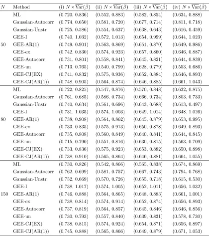
Table 3.2. N× average estimated variance for ˆβ0 and ˆβ1 by ML, Gaussian-Autocorr, Gaussian-Unstr and GEE methods: data generated from MP model with latent (i) exchangeableR(0.5); (ii) AR(1) R(0.5); (iii) gen-eral autocorrelation matrix A and (iv) unstructured covariance matrix U;
xij ∼ uniform(-1,1); p=2, β0 =0.0, β1 =0.5; observation times d=5; based on 500 iterations.
N Method (i)N× ̂Var(βˆ) (ii)N× ̂Var(βˆ) (iii)N× ̂Var(βˆ) (iv)N× ̂Var(βˆ)
ML (0.720, 0.836) (0.552, 0.883) (0.582, 0.854) (0.634, 0.888)
Gaussian-Autocorr (0.774, 0.650) (0.581, 0.720) (0.677, 0.714) (0.811, 0.718)
Gaussian-Unstr (0.725, 0.586) (0.554, 0.637) (0.638, 0.643) (0.616, 0.459)
GEE-I (0.740, 1.032) (0.572, 1.013) (0.654, 0.999) (0.644, 1.023)
50 GEE-AR(1) (0.749, 0.901) (0.563, 0.869) (0.651, 0.870) (0.649, 0.986)
GEE-ex (0.742, 0.830) (0.574, 0.923) (0.657, 0.860) (0.646, 0.887)
GEE-Autocorr (0.731, 0.801) (0.558, 0.841) (0.645, 0.821) (0.644, 0.839)
GEE-un (0.713, 0.765) (0.540, 0.799) (0.628, 0.779) (0.553, 0.686)
GEE-CJ(EX) (0.741, 0.832) (0.575, 0.936) (0.652, 0.884) (0.646, 0.893)
GEE-CJ(AR(1)) (0.748, 0.905) (0.564, 0.874) (0.646, 0.885) (0.661, 1.043)
ML (0.722, 0.825) (0.547, 0.876) (0.570, 0.848) (0.632, 0.875)
Gaussian-Autocorr (0.761, 0.685) (0.586, 0.734) (0.666, 0.734) (0.803, 0.733)
Gaussian-Unstr (0.740, 0.634) (0.561, 0.696) (0.643, 0.688) (0.613, 0.497)
GEE-I (0.731, 1.035) (0.574, 1.003) (0.649, 1.014) (0.648, 1.026)
80 GEE-AR(1) (0.738, 0.908) (0.564, 0.862) (0.645, 0.879) (0.653, 0.995)
GEE-ex (0.733, 0.835) (0.575, 0.913) (0.650, 0.878) (0.649, 0.893)
GEE-Autocorr (0.735, 0.808) (0.560, 0.849) (0.640, 0.841) (0.644, 0.845)
GEE-un (0.715, 0.790) (0.551, 0.816) (0.630, 0.815) (0.563, 0.709)
GEE-CJ(EX) (0.733, 0.836) (0.575, 0.923) (0.653, 0.882) (0.650, 0.898)
GEE-CJ(AR(1)) (0.738, 0.910) (0.565, 0.864) (0.646, 0.881) (0.664, 1.055)
ML (0.730, 0.826) (0.542, 0.866) (0.565, 0.838) (0.674, 0.869)
Gaussian-Autocorr (0.762, 0.699) (0.581, 0.757) (0.667, 0.743) (0.794, 0.768)
Gaussian-Unstr (0.752, 0.669) (0.570, 0.726) (0.655, 0.718) (0.615, 0.530)
GEE-I (0.738, 1.017) (0.574, 1.005) (0.652, 1.011) (0.656, 1.032)
150 GEE-AR(1) (0.746, 0.888) (0.564, 0.865) (0.648, 0.883) (0.661, 1.001)
GEE-ex (0.738, 0.814) (0.574, 0.914) (0.652, 0.874) (0.656, 0.893)
GEE-Autocorr (0.737, 0.819) (0.564, 0.857) (0.645, 0.846) (0.646, 0.856)
GEE-un (0.730, 0.793) (0.557, 0.840) (0.639, 0.831) (0.578, 0.730)
GEE-CJ(EX) (0.738, 0.815) (0.574, 0.924) (0.654, 0.871) (0.656, 0.897)
GEE-CJ(AR(1)) (0.745, 0.888) (0.565, 0.866) (0.649, 0.879) (0.671, 1.053)
of the variance of ˆβ0 does not seem to differ much irrespective of the data genera-tion mechanism and the method of estimagenera-tion, although, Gaussian-Autocorr seems to produce a larger variance estimate when data are generated using the unstructured covariance matrix.
The simulation study was extended to compare bias and MSE. Again, based on 500 simulated samples, we obtained (a) average bias(θˆi) = ∑500i=1(θˆi−θi)/500 and (b)
N×average MSE ( ∑500i=1(θˆi−θi)
2/500). To save space we only summarize the results
(not given here) of the simulation.
Our simulations show that biases of the estimates by all procedures compared are small. In terms of the MSE, the performance of GEE-I is the worst in general. When data are simulated using unstructured correlation structure, Gaussian-Unstr is the best for the estimation of β1, agreeing with the results shown in terms of estimated variances. For the estimation of β0, no method seems to perform better than any other. For data with other correlation structures there do not seem to be any significant differences in efficiency both for the estimation of β0 and β1.
We conducted a further simulation study to compare these twelve estimators by generating correlated binary data with specified marginal means and correlations (Qaqish, 2003). Simulation results not reported here show similar conclusions.
3.4. Examples
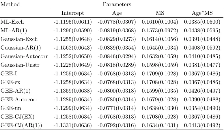
Table 3.3. Results of the regression analysis of the wheezing status data; estimates of β0, β1, β2 and β3 of the model (3.4.1) with standard errors in
parenthesis using maximum likelihood method based on the MP model, four Gaussian estimation methods and six GEE procedures; with probit link.
Method Parameters
Intercept Age MS Age*MS
ML-Exch -1.1195(0.0611) -0.0778(0.0307) 0.1610(0.1004) 0.0385(0.0500)
ML-AR(1) -1.1296(0.0590) -0.0819(0.0368) 0.1573(0.0972) 0.0438(0.0595)
Gaussian-Exch -1.1255(0.0648) -0.0829(0.0273) 0.1614(0.1056) 0.0391(0.0448)
Gaussian-AR(1) -1.1562(0.0643) -0.0839(0.0354) 0.1645(0.1034) 0.0408(0.0592)
Gaussian-Autocorr -1.1252(0.0650) -0.0846(0.0294) 0.1632(0.1059) 0.0410(0.0485)
Gaussian-Unstr -1.1228(0.0649) -0.0818(0.0289) 0.1598(0.1059) 0.0381(0.0477)
GEE-I -1.1259(0.0634) -0.0768(0.0313) 0.1709(0.1028) 0.0367(0.0486)
GEE-ex -1.1258(0.0634) -0.0768(0.0313) 0.1708(0.1028) 0.0367(0.0486)
GEE-AR(1) -1.1359(0.0638) -0.0800(0.0318) 0.1599(0.1035) 0.0426(0.0497)
GEE-Autocorr -1.1289(0.0634) -0.0780(0.0314) 0.1679(0.1028) 0.0390(0.0488)
GEE-un -1.1299(0.0634) -0.0771(0.0314) 0.1638(0.1030) 0.0354(0.0490)
GEE-CJ(EX) -1.1258(0.0634) -0.0768(0.0313) 0.1708(0.1028) 0.0367(0.0486)
GEE-CJ(AR(1)) -1.1331(0.0636) -0.0792(0.0316) 0.1634(0.1031) 0.0413(0.0492)
child at each occasion. The purpose of the study is to model the probability of the wheezing status as a function of the child’s age, his/her mother’s maternal smoking habit (a binary variable MS with 1 if the mother smoked regularly and 0 otherwise) and their interactions. We consider the same marginal model used by Fitzmaurice and Laird (1993) with a probit link
probit(µ) =β0+β1Age+β2MS+β3Age*MS, (3.4.1)
where ‘age’ is the age in years since the child’s 9th birthday.
Estimates of the regression parameters of model (3.4.1) and their standard errors by all the methods discussed are given in Table 3.3. Estimates of the correlation parameters by all the methods are given in Table 3.5.
the standard errors of the estimates by all other methods. For β1 and β3, it appears that the estimates by the Gaussian estimation procedures, except Gaussian-AR(1), produce the smallest standard errors, providing some support that the estimates of the regression parameters by the Gaussian estimation procedure using the general autocorrelation structure and unstructured correlation have the highest efficiency.
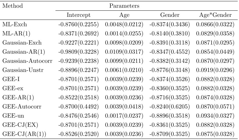
Example 2: The second example uses a subset of the data from the Coronary Risk Factor Study by Woolson and Clarke (1984). The dataset contains records of 1014 children from Muscatine, Iowa, who were 7-9 years old in 1977. Height and weight were measured on each child in three survey years, 1977, 1979 and 1981. For each survey year, the median weight was calculated for each gender and 1 inch of height. Children with relative weight greater than 110% of the median weight in their respective stratum were classified as obese. The repeated binary response of interest is whether the child is described as being obese or not (1=yes, 0=no) at each occasion. Data on many children are incomplete, and only 460 children had complete data from all the three occasions. We analyze only the complete data (see Table 2 in Fitzmaurice, Laird and Lipsit, 1994). One of the objectives of this study was to determine the effects of age and gender on risk of obesity in children. Fitzmaurice, Laird and Lipsit (1994) analyzed these data using a logit link. Here we consider the marginal model with a probit link
probit(µ) =β0+β1Age+β2Gender+β3Age*Gender, (3.4.2)
where Gender=1 if the child is female, 0 otherwise.
Table 3.4. Results of the regression analysis of the complete Mluscatinie Study data; estimates ofβ0,β1,β2andβ3 of the model (3.4.2) with standard
errors in parenthesis using four Gaussian estimation methods and six GEE procedures; with probit link.
Method Parameters
Intercept Age Gender Age*Gender
ML-Exch -0.8760(0.2255) 0.0048(0.0212) -0.8374(0.3436) 0.0866(0.0322)
ML-AR(1) -0.8371(0.2692) 0.0014(0.0255) -0.8140(0.3810) 0.0829(0.0358)
Gaussian-Exch -0.9227(0.2221) 0.0098(0.0209) -0.8391(0.3118) 0.0871(0.0295)
Gaussian-AR(1) -0.9809(0.3228) 0.0109(0.0317) -0.8347(0.4552) 0.0854(0.0449)
Gaussian-Autocorr -0.9239(0.2238) 0.0099(0.0211) -0.8382(0.3142) 0.0870(0.0297)
Gaussian-Unstr -0.8896(0.2247) 0.0061(0.0210) -0.8776(0.3148) 0.0919(0.0296)
GEE-I -0.8701(0.2571) 0.0039(0.0239) -0.8374(0.3526) 0.0882(0.0328)
GEE-ex -0.8701(0.2571) 0.0039(0.0239) -0.8360(0.3525) 0.0882(0.0328)
GEE-AR(1) -0.8522(0.2518) 0.0039(0.0236) -0.8716(0.3525) 0.0874(0.0328)
GEE-Autocorr -0.8700(0.4492) 0.0039(0.0418) -0.8240(0.6205) 0.0870(0.0571)
GEE-un -0.8476(0.2546) 0.0017(0.0237) -0.8896(0.3518) 0.0934(0.0327)
GEE-CJ(EX) -0.8701(0.2571) 0.0039(0.0239) -0.8361(0.3525) 0.0882(0.0328)
GEE-CJ(AR(1)) -0.8526(0.2520) 0.0039(0.0236) -0.8709(0.3525) 0.0875(0.0328)
errors of the estimates of all regression parameters by Exch, Gaussian-Autocorr and Gaussian-Unstr are the smallest.
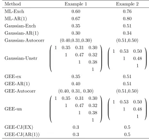
Table 3.5. Estimates of the correlation parameters by different methods for the two examples.
Method Example 1 Example 2
ML-Exch 0.60 0.76
ML-AR(1) 0.67 0.80
Gaussian-Exch 0.35 0.51
Gaussian-AR(1) 0.30 0.34
Gaussian-Autocorr (0.40,0.31,0.30) (0.51,0.50)
Gaussian-Unstr ⎛ ⎜ ⎜ ⎜ ⎜ ⎜ ⎝
1 0.35 0.31 0.30
1 0.47 0.32
1 0.38 1 ⎞ ⎟ ⎟ ⎟ ⎟ ⎟ ⎠ ⎛ ⎜ ⎜ ⎜ ⎝
1 0.53 0.50
1 0.48 1 ⎞ ⎟ ⎟ ⎟ ⎠
GEE-ex 0.35 0.51
GEE-AR(1) 0.40 0.51
GEE-Autocorr (0.40, 0.31, 0.30) (0.51,0.50)
GEE-un ⎛ ⎜ ⎜ ⎜ ⎜ ⎜ ⎝
1 0.35 0.31 0.30
1 0.47 0.32
1 0.38 1 ⎞ ⎟ ⎟ ⎟ ⎟ ⎟ ⎠ ⎛ ⎜ ⎜ ⎜ ⎝
1 0.53 0.50
1 0.48 1 ⎞ ⎟ ⎟ ⎟ ⎠
GEE-CJ(EX) 0.3 0.5
GEE-CJ(AR(1)) 0.3 0.5
3.5. Discussion
In this chapter, we developed a Gaussian estimation procedure involving a work-ing correlation matrix for the estimation of the regression parameters in longitudinal binary response data. It is interesting to see that the first part of the Gaussian score function (3.2.2) is the GEE function and the second part can be regarded as a correc-tion term for obtaining estimates of regression parameters with higher efficiency. To preserve the (asymptotic) unbiasedness of the Gaussian estimating equations (3.2.3), the second part of (3.2.2) should be convergent to zero asymptotically. For this pur-pose, we prefer to choose working correlation matrices with robust structures.
irrespective of whether the true correlation structure is unstructured, general auto-correlation, AR(1) or exchangeable. Thus, the Gaussian estimates of the regression parameters using an unstructured working correlation matrix do not suffer from the pitfalls that Crowder (1995, p. 408) discusses regarding the GEE estimates. Fur-ther, the estimates of the regression parameters and the correlation parameters of the working correlation matrix are consistent when the working correlation matrix consid-ered is general autocorrelation irrespective of whether the true correlation structure is general autocorrelation, AR(1) or exchangeable. In this sense the unstructured corre-lation matrix is most robust against misspecification by other correcorre-lation structures. The next most robust is the general autocorrelation structure.
It shows in Section 2.5 that the Gaussian estimating functions can be obtained by an approximation to marginal normal scores on the basis of the deviance residual (see equation (2.5.3)) in the Gaussian copula regression model (Song, 2000). This provides another theoretical justification of the application of Gaussian estimation to longitudinal binary data analysis. Though both Gaussian estimation and Gaussian copula regression model use the density function (or cumulative distribution func-tion) of a multivariate normal distribution, there are two major differences between these two methods. First, the covariance matrix in Gaussian estimation models the correlation between any two response variables directly while the covariance matrix in the Gaussian copula model measures the correlation between two normal scores, Φ−1{G
i(yi)} and Φ−1{Gj(yj)} (see equation (2.5.2)). Second, the joint density