A novel coverage algorithm based on event probability driven mechanism in wireless sensor network

(1)

R E S E A R C H

Open Access

A novel coverage algorithm based on

event-probability-driven mechanism in wireless

sensor network

Zeyu Sun

1,2

, Weiguo Wu

1

, Huanzhao Wang

1*

, Heng Chen

1

and Xiaofei Xing

3

Abstract

Coverage problem is an important research topic in the field of wireless sensor network (WSN). The coverage algorithm based on event probability driven mechanism (EPDM) is put forward in this paper. First of all, the network probability model is established and the subordinate relation between sensor nodes and the target nodes is presented. Secondly, a series of probability is computed and the related theorems and reasoning are also proven. Thirdly, effective coverage for the monitoring region is achieved through scheduling mechanism of nodes themselves, thus the purpose of increasing network lifetime can be realized. Finally, experimental results show that the proposed algorithm could achieve complete coverage for networks of different scale and increase the network lifetime. It possesses the good quality of effectiveness and stability.

Keywords:Wireless sensor network; Event probability; Coverage algorithm; Sensor nodes

1 Introduction

Wireless sensor network (WSN) is a wireless distributed network system, composed of large amount of self-organized microsensor nodes which are integration of data collecting, processing and transmission units and power supply units, and performing the functions of information collecting, data processing, and transmission. What is more, WSN is mainly applied in the field of military defense, environment monitoring, medical care, intelligent home, agriculture, and transportation, etc. WSN compromises the information world and physical world and changes the interactive mode between the nature and human being [1-3]. At present, WSN has received the attention from all fields and brought immeasurable benefits to the society. Besides, it arouses the research warmness for WSN technology. WSN works in poor environment in which sensor nodes are usually deployed in the monitoring region through random spreading [4,5]. Distribution of sensor nodes is very uneven. The energy of it is limited and cannot be recharged. Therefore, it needs considering first to prolong the network life by adopting effective

energy-saving coverage method and energy-consuming balance mechanism in the research and designing of WSN [6-8]. In wireless sensor networks, the ultimate goal of coverage is to allocate each node's state efficiently, minimize the network's energy consumption in each cycle, and balance the share of each node's energy con-sumption in the network without reducing the existing level [9]. The coverage directly reflects the capability of network to monitor the physical world, and energy consumption determines the lifetime of the wireless sen-sor networks. Network coverage and energy consumption are closely related.

According to the mobility property of the node, the coverage problem that is an important topic in the wire-less sensor network can be divided into two classes: static nodes and mobile nodes [10,11]. Therefore, according to the constitution of nodes, WSN can be divided into two types: static and mobile. A hybrid WSN can be established by mixing the static and mobile nodes in the same WSN. The static sensor network refers to the network composed of only static nodes. Its cost is low. But the static nodes have many limitations and cannot meet the requirement of actual application. The mobile sensor network is composed of only mobile nodes and has good mobility. However, the mobile nodes usually undertake more tasks

* Correspondence:[email protected] 1

School of Electronics and Information Engineering, Xi’an Jiaotong University, Xi’an, Shaanxi Province 710049, China

Full list of author information is available at the end of the article

(2)

than static ones and are equipped with special mobility modules. Thus, the components of mobile nodes are much stronger than static ones. Big size and high cost make it less possible to apply in the real situation. The hybrid sensor network is constituted of both static and mobile nodes. Its advantages include low cost, good mobility, and the most frequent application.

The structure of hybrid sensor network is almost identical with WSN, but a certain amount of mobile sensor nodes with mobility property makes the cost slightly higher than traditional WSN. However, the number of mobile nodes can be set according to specific application, and the cost can be limited in the affordable range. Due to the merits of hybrid sensor network, the related researches are more than other researches. More often than not, hybrid sensor networks are studied in the research of WSN, such as coverage and connectivity, loca-tion, routing, data fusion, etc. All the problems in the networks can be solved in better ways in hybrid sensor networks by using the mobile nodes, such as coverage. If mobile nodes in mobile sensor network are relocated, the nodes can be distributed more evenly and the coverage hole can be filled. By this way, the quality of coverage in the network can be improved.

The rest of this paper is organized as follows. (1) After related literature is reviewed, the main idea of coverage algorithm is introduced. Based on event probability, the model of WSN is established. (2) The process is verified through function relationship of Poisson distribution, normal distribution, and the probability density for the edge nodes in the WSN. (3) The coverage rate under certain condition can be determined through the state transition of nodes and the associated attributes between sensor nodes and target nodes. Therefore, the overhead of node energy can be decreased and dynamic allocation can be achieved. (4) As to network energy, the targets in concern are always located in the sensing range of the working nodes by employing the dynamic allocation mechanism. The state transition of nodes can be finished through scheduling mechanism; thus the dynamic adjust-ment of nodes can be realized. The overall network energy can be kept in balance. (5) In the final part of this paper, the schematic diagram of coverage rate and network energy changing with time under different variable system through simulation is presented. The study process is summarized, and the future work is forecasted.

2 Related works

A lot of studies and verifications have been done on the coverage algorithm of WSN in recent years in China and abroad. A superimposed cycle was established by means of semi-Markov, and the network model was constantly updated. When the target was covered by several sensor nodes, the target should be ensured to be covered by at

(3)

required [21]. As for target coverage, what we should resolve is thatmtargets of known position were given and n monitoring nodes were deployed. Due to the limited energy of every sensor node, it was a problem on how to deploy nodes in a reasonable range and how to maximize the network lifetime on the basis of target monitoring. Cardei and Du put forward a heuristic algorithm by using mixed integer programming [22]. Then, they discussed the coverage problem in the case of node sets intersection and adjustable sensing radius of node. When the targets' density was high, Cardei ap-proximated the target coverage as region coverage and realized the connectivity coverage of the target through establishing a connected set of nodes with the help of sensing nodes in high density. Based on the studies of Cardei, Liu and other researchers further studied the target coverage problem. He constrained one node to cover only one target each time [23]. It could be ensured that target coverage problem could be resolved effectively in polynomial time. Wu et al. proposed a protocol which constructed distributed localization of connected dominat-ing set and discussed methods of dominatdominat-ing set coverage with efficient energy. To balance the network energy consumption, a method of selection coverage nodes was presented through remaining energy level [24]. Through the above methods, only static nodes were used to cover the target continuously, but in some applications, it was not necessary to provide continuous coverage of target. It would be much more efficient to use some of mobile nodes than just use static nodes. A polynomial approxima-tion algorithm was presented by constructing a minimum spanning tree [25]. It was also discussed how to reduce the number of nodes and how to determine the position of nodes to cover a given target in the secure and control-lable network environment. In addition, the connectivity of network must be ensured [26].

3 Statement of the problem and the network model

For the convenience of study, the algorithm in this paper is based on the following four assumptions:

(1) The communication range and sensing range of wireless sensor nodes are disc-shaped. The position of each node can be obtained through some positioning algorithm.

(2) The nodes in the WSN are morphologic and independent. Each node has the same sensing range but different communication range.

(3) All the nodes in WSN are randomly deployed in a square area. The border factor and the condition in which the border exists should also be considered.

(4) At first, each node has the same energy and they are in the same status in the network.

3.1 Basic definitions

Definition 1 The fact that some area is covered by the node si means any point p in this area is within the

coverage of si. That is: Asi= {p|d(p, (x, y))≤rs, i∈[1, n]}.

d is the Euclidean distance between two points. rsis the

sensing radius of nodes. n is the number of nodes. Definition 2The coverage rate of WSN in W deployed in target area Ω, is Ci(W,Ω) =∫ Ωs(xi)dx/S(Ω). S(Ω) is

the area of the target region, when D(si, tk)≤1, S(Ω) = 1,

otherwise, S(Ω) = 0.

Definition 3There exist node siand sj. The target regions

they covered are Ωi and Ωj, respectively. ifΩi ∩ Ωj≠ ∅,

then node siand sjis regarded to be coverage related.

3.2 Network model

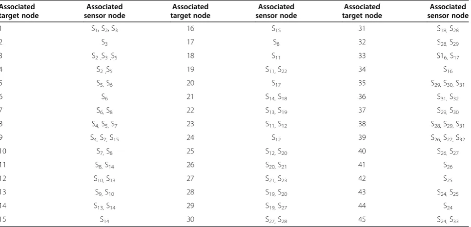
For the sake of convenience, the sensor nodes and the target nodes are placed in a square region. Generally, the coverage level of the target directly reflects the level that the target node is concerned. The target node region being concerned has a higher coverage level. The function of expectation value of different areas where the sensor node P is located and the coverage area should be taken into consideration, as is shown in Figure 1.

Figure 1 shows the associated coverage relationship of sensor nodes and target nodes. Circles represent the sensor nodes; triangle represents the target nodes; dot-ted lines in the figure represent moving locus of mobile targets. In the lower left corner, node P is defined. Shadows are blind regions which are not covered by sensor nodes. When the target node moves from the upper left to lower right of the figure to the sensor nodes 9 and 11, some region cannot be covered. We call it empty or blind area. In Figure 1, four problems are studied as follows:

(1) What is the relation of the associated attributes between wireless sensor nodes and target nodes? (2) For target nodes, how to denote the relationship of

wireless sensor nodes and the target nodes? (3) What is the relationship between the area of blind

region and that of wireless sensor nodes? (4) How to compute the coverage level, density

functions, and the expectation value of the nodes in WSN?

(5) How to determine the coverage of target area with the least deployed nodes by using the probability expectation value? How to realize scheduling mechanism of sensor nodes?

(4)

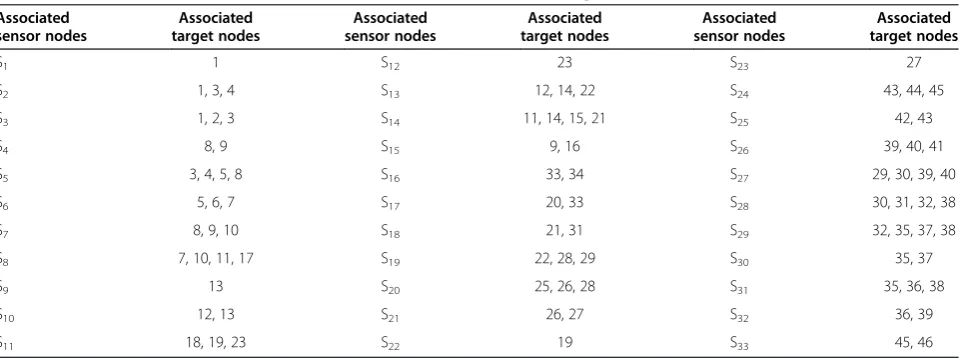
more than one sensor nodes, namely, K degree coverage. A chart is used to represent the associated attributes between WSN nodes and the target nodes, as shown in Table 1.

From Table 1, we can see that each target node is covered by one or more sensors, and the coverage degree for each target node is not the same. When the target node is covered by multiple sensor nodes, it may be the main target node being concerned, but if it is covered by

multiple sensor nodes (K≧2), it may not be the one being concerned. Some sensor nodes can be put into a dormant state in order that the energy consumption of the sensor nodes can be reduced. This will be further explained in the subsequent chapters.

The second problem is exactly the inverse problem of the first one. That is, a target node is covered by multiple sensors and the K degree coverage is formed. The formed association relationship between this target Figure 1Schematic for associated coverage attribute.

Table 1 The associated attributes between wireless sensor nodes and target nodes

Associated sensor nodes

Associated target nodes

S1 1 S12 23 S23 27

S2 1, 3, 4 S13 12, 14, 22 S24 43, 44, 45

S3 1, 2, 3 S14 11, 14, 15, 21 S25 42, 43

S4 8, 9 S15 9, 16 S26 39, 40, 41

S5 3, 4, 5, 8 S16 33, 34 S27 29, 30, 39, 40

S6 5, 6, 7 S17 20, 33 S28 30, 31, 32, 38

S7 8, 9, 10 S18 21, 31 S29 32, 35, 37, 38

S8 7, 10, 11, 17 S19 22, 28, 29 S30 35, 37

S9 13 S20 25, 26, 28 S31 35, 36, 38

S10 12, 13 S21 26, 27 S32 36, 39

(5)

node and sensor nodes will be studied in the second question. The association relationship between target nodes and sensor nodes is shown in Table 2.

From Table 2, we can see that each target node is cov-ered by one or more sensors and the coverage degree for each target node is not the same. When a target node is covered by multiple sensor nodes, multiple coverage is formed. For example, target node 8 is in the coverage range of S4, S5, S7and the degree of the coverage is 3. If

the coverage degree for a target node is higher than needed, there must exist many redundant nodes. This will consume much energy of the entire network, and the network lifetime will be decreased. With the increasing of sensor nodes, more than one target nodes are most likely to be in the multiple coverage area. Large sum of redun-dant nodes will be generated with the precondition that a certain coverage degree can be realized. In order to avoid the existence of many redundant nodes, all the sensor nodes should be put in different states and the transition of different states should be accomplished.

3.3 The formation and calculation of the curve locus

Definition 4Given the target set T = {t1, t2, t3…tk} and

sensor node set V = {v1, v2, v3 … vn} in a certain time

slot, if any node tkin target set T is covered by at least

one node in node set V, then it is called full coverage of target set T.

Definition 5 Let T be the set of m nodes distributed randomly in the target area. Let E be the edge set of the network graph, which represents set of positional relation-ship of eij: ei= tj. eijindicates the position of node si and target node tj. When ei= 1 if and only if the Euler distance

between target nodetjand sensor nodesi is less than or equal with the sensing radius ri, otherwise ei= 0. W = {w1,

w2⋯wn} is the initial energy set of the sensor nodes. W

conforms to W∼N(u, σ2) normal distribution. wi

repre-sents the initial energy of sensor node si, and wi is the

maximum energy in the working process of nodes. The third and the fourth problem are studied together. As for the area of the shadow, what should be consid-ered is changing the function model of mobile target nodes' walking trajectory and the function relationship between sensor node 9 and sensor node 11. Through data fitting for the moving path of mobile nodes, the function of mobile target nodes' walking track is given as follows:

f1ð Þ ¼x anxnþan−1xn−1þan−2xn−2þ⋯þa1x1þξ ð1Þ

Let a be in the range between 0 and 1, i.e., a∈ [0, 1]. To calculate the area of the shadow, it is intercepted in Figure 1 and a two-dimensional plane with X-axis and

Y-axis is established. The shadow, part of the figure of sensor node 9 and 11, and sensor node 30 in the lower left corner of Figure 1 are shown in Figure 2.

In Figure 2, the X and Y-axes are made through the center of node 9 and 11. The point of intersection is the original point. Let a and b be the center of the sensors 9 and 11, respectively. Connect a and b. Let c be the cut point, e be the intersection point ofX-axis and the walk trajectories of moving target nodes, and d be the intersec-tion point of Y-axis and the walk trajectories of moving target nodes. The coordinates of the point a are (xa, 0),

the coordinates of point b are (0,yb). Because point c

Table 2 The coverage association between wireless sensor nodes and target nodes

Associated target node

Associated sensor node

1 S1, S2, S3 16 S15 31 S18,S28

2 S3 17 S8 32 S28,S29

3 S2 ,S3 ,S5 18 S11 33 S16,S17

4 S2 ,S5 19 S11,S22 34 S16

5 S5,S6 20 S17 35 S29,S30,S31

6 S6 21 S14,S18 36 S31,S32

7 S6,S8 22 S13,S19 37 S29,S30

8 S4,S5,S7 23 S11,S12 38 S28,S29,S31

9 S4,S7,S15 24 S12 39 S26,S27,S32

10 S7,S8 25 S12,S20 40 S26,S27

11 S8,S14 26 S20,S21 41 S26

12 S10,S13 27 S21,S23 42 S25

13 S9,S10 28 S19,S20 43 S24,S25

14 S13,S14 29 S19,S27 44 S24

(6)

is the outer cutting point of sensor node 9 and 11, the coordinates of c are (0.5x, 0.5y). The coordinates of point e are (xa+r, 0). The coordinates of point d is (0, yb+r). The shadow area is the enclosure of mobile

tar-get nodes withX-axis andY-axis minus the area of the bottom corner and the circle. As for the area of the bottom corner, curve equation can be presented by means of data fitting. Let b∈[0, 1], the curve equation is as follows:

f2ð Þ ¼x bnxnþbn−1xn−1þbn−2xn−2þ⋯þb1x1þξ ð2Þ

The area of the shadow is as follows:

S¼ Z xaþr

0

f₁ð Þx dx− Z xa−r

0

f₂ð Þx dx−πr2 ð3Þ

With formula (1) and formula (2) into formula (3), the result is as follows:

S¼ 1 iþ1

Xn

i¼1

aiðxaþrÞiþ1−biðxa−rÞiþ1

h i

−πr2 ð4Þ

Theorem 1 Without loss of generality, if the empty hole exists and its curvesf(x) andg(x) are continuously differentiable, then the absolute value of its empty area

difference is not less than the sum of the area of the two fan-shaped out-cut regions.

Proof As is shown in Figure 2, the X-axis and Y-axis

coordinate is moved horizontally to o′, and a new coordinate X′-axis and Y′-axis is formed. The sensor node 9 and Y′intersect at m and n, where the angle formed is β; similarly, the sensor node 11 and the axis X′intersect at point g and f. Its angle formed is α. Because the empty hole exists S≥0, ΔS = |S1−S2−Sfan|≥0, ac-cording to formula (3) and (4), the following result can be conducted:

ΔS¼ 1 iþ1

Xn

i¼1

h i

−Sfan ð5Þ

When Sfan ¼2πr2−1₂r2ðαþβÞ is put into formula (5),

the result is as follows:

ΔS¼ 1 iþ1

Xn

i¼1

h i

−Sfan

¼ 1

iþ1 Xn

i¼1

h i

−2πr2−1 2r

2_ð_α_þ_β_Þ

(7)

Because of the existence of the empty hole, there exists ΔS≥0. Consequently, the ultimate result is con-ducted as follows:

From theorem 1, the conclusion can be drawn: if {0≤α≤π} ∩ {0≤β≤π}, the area of the empty hole needed to fill is at least 2πr2. If anglesα and βare in the range of [π, 2π], the area needed is at leastπr2.

Theorem 2Without loss of generality, if the holes exist, i.e., x≥0 and is continuously differentiable in the range of [0, a]. Besides, if the track equation of the hole satisfies

f_nð Þ ¼x

solute convergence in the range of [0, a].

Proof Because x≥0 and it is continuously differentiable in [0, a], |f0(x)| is continuous in [0, a] and there is the

maximum value of |f0(x)| in the range of [0, a]. LetM be

the maximum value,M¼ max

0≤x≤ajf0ð Þx j. Because:

Because |f0(x)| is continuous in [0, a], there exists the

maximum value,Mof |f0(x)| in [0, a]. Consequently:

fnð Þx

Because formula (9) is convergent when x ∈ [0, a], X∞

3.4 Coverage area and its expectation value

In the following sections, the relationship between the coverage area and its expectation value is analyzed through the example of sensor node 30 (node p) in the lower left corner.

A is shown in Figure 2; the square region l is divided into two parts: region I and region II. The nodes are ran-domly deployed in the monitoring region and constituted in a limited set S. The coverage area of each node is E (C). The coverage probability of each node is E(C)/Ω. If S is empty, the coverage rate of the deployednnodes is P(S) = (1–E(C)/Ω)n. When set S is not empty, the value of coverage probability of network nodes is as follows:

P Sð Þ ¼1−ð1−E Cð Þ=ΩÞn ð10Þ

When node number n→∞, lim

n→∞E P Sð ð ÞÞ ¼1 . This means that when the number of nodes is large enough, the monitoring region will be fully covered. Considering the boundary effect, the node coverage area and its expectation value is to be solved. Because the square region is divided into regions I and II, according to the definition of expectation value in probability theory, the expectation value of nodes coverage area in the network can be conducted as follows:

E Cð Þ ¼Pð ÞΩΙ E Cð ΩΙÞ þPðΩΙΙÞE Cð ΩΙΙÞ ð11Þ

P(Ω_Ι) and P(Ω_ΙΙ) denote the probability of the node randomly deployed in region I and region II, respectively.

E Cð ΩΙÞandE Cð ΩΙΙÞrepresent the corresponding coverage expectation, respectively. Because the deployment of sensor nodes follows uniform distribution, thereby the following result is obtained:

Pð Þ ¼ΩΙ ðl−2rsÞ2=l2 PðΩΙΙÞ ¼4rsðl−rsÞ=l2

ð12Þ

Assuming node p is inside regionI, its coverage range is completely contained, so the coverage expectation is as follows:

E Cð ΩΙÞ ¼πr2s ð13Þ

When node p is inside region II, the area is that of its sensing circle minus that of arch regionSACBD. A and B

is the intersection of the sensing circle of node p and the network border. Its angle θ is the central angle formed by node p, point A and point B, i.e., ∠ApB =θ.

Theorem 3 Supposing that the given sensor nodes

with sensing radius rs are uniformly distributed in the

square region with side length of l, considering the

boundary factors, the coverage expectation of each node is as follows:

ProofBecause the sensor nodes follow uniform

(8)

E Cð Þ ¼Pð ÞΩΙ E Cð ΩΙÞ þPðΩΙΙÞE Cð ΩΙΙÞ. When formulas (12), (13), and (14) are put into formula (11), the result is as follows:

Theorem 4 Given a square region with side length l,

sensing radius of node r and smaller parameter ε, in

order to ensure that the expectation of network coverage is not less than ε, the number of nodes to be deployed is at least: ln(1−ε)/ln(1−E[C]/Ω).

Proof According to formula (1), P(Sn) = l−(l−E[C]/

Ω)n≥ε, then the result can be obtained: n ln(1−E[C]/ Ω)≤ln(1−ε). Because ln(1−E[C]/Ω) < 0, n≥ln(1−ε)/ln (1−E[C]/Ω).

Deduction 1For any value of stochastic variable X in the range [a, b], the mathematical expectation and variance of bounded stochastic variable always exists.

Proof Because the stochastic variable X can get

any value in [a, b] and its expectation should also be in [a, b], p(x) as the density function of X, ac-cording to expectation formula, the following result can be obtained: According to definition of variance and formula (16), the following result can be obtained:

Var¼E Xð −E Xð ÞÞ2≤E X −aþb ₂2≤E b −aþb ₂2 ¼ b−a

2

ð17Þ

That is to say, its expectation and variance both exist for any bounded stochastic variable.

4 Sensing probability model and the node scheduling mechanism

Two ways are usually adopted for measuring sensor models: one is sensing model method, and the other is the probability model method. Currently, the latter is studied more than others. An important factor for sensor model is the size of coverage for the monitoring region. It is mainly reflected by coverage rate.

4.1 Probability model of node

From definition 5, coverage rate of the point si in the region is as follows:

When the target node is in the monitoring area and lies in the position (xt−x)2≤r2, its probability of being

covered is 1 and vice versa. When the target node is near the border of the sensing node or less than the maximum radius rmax, its coverage probability is e−λd. d

is the Euler distance between target node and sensor node. The major impact of the border on the coverage is that the number of nodes should be increased to cover it if the target node is near the border of the coverage area. Such coverage follows nearby covering principle, i.e., when the Euler distance of a sensor node and the target node is short, the node moved in a straight line through certain moving strategy to realize coverage. If the Euler distance between the target node concerned and the border node is less than or equal to the diameter of the sensor node, coverage can also be realized through moving sensor nodes. If the Euler distance between the target node con-cerned and the border node is larger than the diameter of the sensor node, the only way to cover the border target nodes is to schedule nodes near the target node.

Definition 6 The mobile node i is at the point of xi.

Another mobile node j is at the point of xj. The repulsive

force of j to i is defined as:

Similarly, the attraction of j to i is defined as:

Fatt¼ k

In the formula above, k is a proportionality constant coefficient, repulsive and attractive forces are as follows:

F¼

As to the limitedness of coverage area, the repulsive force of target area border from the mobile node can also be applied to other models. This time, the point xjis the

(9)

the random disturbance force between nodes, the resultant force at a node is as follows:

Fi¼ X

ξ1Fexcþξ2Fattþξ3Fborþξ4Fwan

ð Þ ð22Þ

Fbor is the repulsive force of target area border from the mobile node. Fwan is the random disturbance force between nodes. ξ is the force control parameter. The equation of the mobile node i at the time of t can be defined as: v″ð Þ ¼x Fi−μx′i=m

. μ is the proportional damping factor, m is the node's virtual mass.

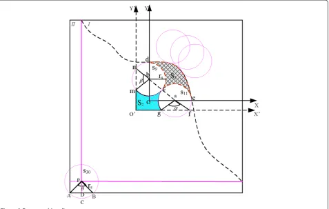
Because sensor node 1 covers one target node con-cerned and the Euler distance between the target node and the border node is larger than the diameter of sensors node 1, only sensor node 2 or sensor node 3 can be moved. Because L2 > L3 and both sensor nodes 2 and 3 have not concerned the target node, sensor node 3 should be moved. The dotted line is the shortest distance between the target node and sensor node 3, as shown in Figure 3.

As can be seen in Figure 3, the target node lies in be-tween r and rmax, which also shows the only possibility

of existence of the boundary target node (triangles are the target nodes). For more complex network models, the probability model is transformed into a normal distri-bution function. X follows normal distridistri-bution, represented

as X∼N(μ,σ2). u is the expectation of normal distribution, and σ2is the variance of the normal distribution. That is as follows:

p xð Þ ¼ ffiffiffiffiffiffi1 2π p

σe −ðx−uÞ2

2σ2 ð₂₃Þ

Deduction 2 Let stochastic variable X follow normal distribution N∼(μ, σ2). If p(a≤X≤b)≥99% is required, solve the function relation of parameters.

ProofFrom known conditions,

p að ≤X≤bÞ ¼ϕððb−μÞ=σÞ−ϕðða−μÞ=σÞ≥99% ð24Þ

We regard it as complete coverage if the probability is larger than 99%. The effective coverage for the monitoring region is realized.

Assuming a = 0, b = 100,μ= 50, after those parameters substituted into formula (23), the value ofσ is obtained through calculations:σ= 19.41. That is, complete coverage is realized in the monitoring region [0, 100],σ= 19.41.

Deduction 3Ifnsensor nodes was randomly deployed in the network region with area ofΩand the node sensing radius is rs, the probability of K nodes in the region with

area ofπr2

sis as follows: Nπr2s

k

e−Nπr

2 s Ω =ΩkK!

Proof According to Poisson theorem, when the number

of sensor nodes N tends to infinity, the probability P tends

(10)

to be infinitively small. The secondary distribution of term B(n, p) Poisson distribution can be approximated as p(n, λ). Let λ= np. All the sensor nodes in the network coverage area are randomly deployed, so the number of nodes in the network coverage region with area of πr2_s can be considered to follow the secondary distribution of B n;πr2

s=Ω

. Because high-density de-ployment is usually adopted to deploy senor nodes in coverage region and the sensing radius of each sensor node is much smaller than the area of the network regionΩ, when the number of nodes n in the coverage area increases gradually, nπr2

s=Ω is gradually close to infinitive small. The binomial distribution can be ap-proximated as the Poisson distribution p n;nπr2

s=Ω

. In other words, the probability of K the coverage rate of any point in the network coverage is P =λke− λ/k ! with K∈N.

Definition 7Undirected communication diagram G = (V,E) is used as the model of WSN. V is the set of sensor nodes and |V| = n. If and only if nodes p and q are within the communication range of each other, it is regarded that there exists an unidirectional edge (p, q) in E. The number of neighbor nodes of node p is called the degree of node p, represented as d(p) showing the number of nodes that node p could communicate with directly. The minimum node degree of communication diagram G is represented as dmin(G) = min∀p∈V{d(p)}.

Definition 8If there exists a path for any pair of nodes communication diagram G, then the network is called connected. Otherwise, it is not connected. For a connected network, all of its nodes can communicate with each other through one or more hops. On the contrary, there exist some isolated sub-networks in an unconnected network. Its nodes constitute sub-networks that can communicate in themselves. However, the inter-communication among those sub-networks is impossible.

According to definition 6 and definition 7, dmin(G)> 0

is a necessary condition instead of a sufficient condition that communication graph G is connected. So P(Cn)≤P

(dmin(G) >0). In the application, the lower limit of P(Cn)

is of greater significance in the case of unknown node density. If the network communication diagram is con-structed from the empty graph with only isolated nodes, the number of communication links increases while the node communication radius is increased. When the node obtains the minimum node degree k, it has also become a k-connected graph. If any k-1nodes are removed from the network diagram and this graph is still connected, it is called k-connected graph. There-fore, for k =1, as long as its communication radius is large enough to make dmin(G) > 0, the network has be-come a connected network, i.e., P(Cn) = P(dmin(G) > 0). Because the node distribution is independent, according to formula (1), for any node p and (P∈G), the limitation

of the node connectivity rate is lim

n→∞ 1− 1−

According to the literature, the minimum node degree of G is as follows:

Sp is the effective communication area. Without

considering the effect of boundary factors, P Cð Þ ¼n P

dminð ÞG >0

communication circle of node p. When node p is inside the area II, the value of Spis equal to the communication

circle areaπr2_t minus the area of arch SACBD, so:

Assuming node q lies on the border of square deployment region and Sp> Sq,Sq ¼πr2t=2, so:

Theorem 5Given a square region with side lengthl, the

number of nodes in the region isnand the communication

radius of each node is rt. When the boundary effect is

con-sidered, the lower bound of the network connection

prob-ability is P Cð Þn > 1−e−nπr

(dmin(G) > 0); it can be solved. According to deduction 2, if l= 100 m,rt= 40 m,and the boundary effect is

consid-ered, the network is fully connected when the probability of connecting the network is greater than 99% with 124 nodes deployed.

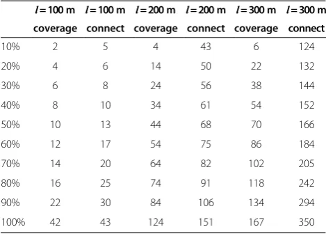
In order to achieve different coverage of network and connectivity rate, the number of nodes to be deployed is shown in Table 3. In this table, the value of the number of nodes to be deployed can be found. When the network coverage and connectivity rate is high (usually≧99%), the network can be considered to be completely covered and connected. When the network connectivity rate P(Cn) is

equal to the network coverage rate E(Sn), more nodes

(11)

4.2 Scheduling mechanism of nodes

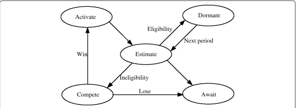
The length of WSN lifetime mainly depends on the en-ergy consumption of nodes themselves and the outside factors. Effective constrain of node energy consumption can prolong the life cycle of the whole network. That re-fers to the fifth question [27,28]. Each sensor node shifts its working status in a certain cycle. At the beginning of each working cycle, the state information of the sensor nodes is initialized, including closing sensing modules of nodes, updating the location of nodes themselves and the neighbor nodes [29]. At any time, the sensor nodes in the network are in one of the following five states: judging, competing, waiting, starting, and sleeping. The connotations of the five states are as follows. The first one is judging: to judge whether it is suitable for sleep-ing. If it is (Eligibility), then it will go in sleeping; other-wise (Ineligibility), it will be delayed randomly for nodes deployment. The timer is started to get ready for the competing state. The second one is competing: if the time is out in the timer, the competition of node is successful (Win). Then, it goes into the starting state; otherwise (Lose), it goes into the state of waiting. The third one is the waiting: the failed nodes in competition falls in the state of waiting and receives the broadcast ‘On-duty Message’from the successful nodes. Then, the nodes entered the state of judging through updating the stored local state information of other nodes so that the coverage judgment algorithms can be contin-ued in the state of judging. The fourth one is starting: the nodes which compete successfully will go into the state of starting. First of all, On-duty Message, including the only ID and location of this node should be broadcasted for other nodes. Meanwhile, the sensing work should be performed. After the starting state, the end of a working cycle, the node initializes the state information and pre-pares for judgment of next working cycle (Next period).

The fifth one is sleeping, unnecessary equipments are turned off for sensor nodes to save energy. After the end of sleeping, the node initializes the state information and prepares for judgment of next working cycle. Each node performs the self-scheduling according to the state of other nodes until it is identified in the state of starting or sleeping, as shown in Figure 4.

4.3 The algorithm and its description

Due to the connectivity of high density sensor nodes and the coverage area of target nodes, the randomly given coverage area is reconstructed through limiting the maximum amount of distortion of randomly covered area in a certain range in order to maximize the life cycle of the network and solve the optimization problem better. At this point, the maximization of the network lifetime is transformed into the problem of target area coverage. In essence, the maximization of the given net-work lifetime is transformed into seeking the largest set of sensor nodes in the entire target area. Each sensor node is related to the specific coverage area required by nodes in the target region. Therefore, the optimization can be solved through coverage theory. After long-time study, many experts and scholars found that there are two main factors affecting the network lifetime: first, the energy consumption of each sensor node in the process of collecting data and, second, the topological geometry of deploying sensor nodes. Due to the transformation from the optimization of network lifetime into the cover-age problem, it is particularly important for sensor nodes to cover specific areas, which is the key to solve the optimization problem. In this paper, we first propose to transform the information collection and data retrieval into energy restriction and coverage-related issues. Second, the given network lifetime maximization prob-lem is determined as a NP-complete probprob-lem. Third, the scheduling mechanism of sensor nodes is trans-formed while the optimal coverage rate is solved through the greedy algorithm. The energy consumption is effect-ively decreased, and the network lifetime is prolonged. The energy consumption of sensor nodes in data retrieval in the whole network system is solved. Finally, the effective-ness and applicability of the algorithm is verified through experimental comparison.

Step 1: Set the position and coverage radius r of sensor nodes. The entire coverage region is divided into multiple disjoint sub-regions {F1, F2 ⋯Fn}. Sensor nodes in every

sub-region Fiand all coverage regions are connected and

guaranteed in the region, i.e., Fl= {Sn1, Sn2 ⋯Snl}, Fl⊂Msi.

Every related subset is marked as Si= {Fn1, Fn2 ⋯ Fnl}

and ∪

i¼1;2⋯nFi¼A.

Step 2: As for the i (i= 1, 2…n) data retrieval, its output is a coverage set: Ci. A concerned sub-region Table 3 Number of nodes to be deployed of different

network coverage and connectivity rate in different network sizes

l= 100 m l= 100 m l= 200 m l= 200 m l= 300 m l= 300 m coverage connect coverage connect coverage connect

(12)

Fc¼ arg min Fl

X

Sni∈Fl

⌊

Ei_r=Ei_c

⌋

is selected.Ei_r is the remaining energy of the i sensor node in the current data collection and retrieval.

Step 3: In order to reduce the amount of overlapping coverage for sparse coverage sub-region caused by the redundant nodes, so an overlap value vi= Fc for the ith

sensor node is defined. It represents the number of sensor nodes and Fc∈Si. viis the number of selected important

sub-areas for the coverage of the ith sensor nodes, i.e., vi= vmin. vminis the minimum number of sensor nodes

in the covered target area.

Step 4: All the sensor nodes in the current coverage area update the remaining energy by reducing the con-sumed energy in the previous data collection and retrieval from the remaining energy, written as Ei_r¼Ei_r−Ei_c. If the remaining energy of a sensor node is less than the required energy for one data collection and retrieval, the sensor node should be removed from the sensor set. Then go to step 2 and continue until coverage region A is not fully covered by sensor nodes available any longer. At this time, the network lifetime is maximized.

4.4 Determination of the node probability

In the designated monitoring area, when any node receives data packets transmitted by the rest N-1nodes, it can be considered to finish data retrieval.

Theorem 6In the wireless sensor network constructed by N wireless sensor nodes of one monitoring area, when there is one and only one sensor node transmitting the

data packet and the probability value of the node pi is

1/N + 1−i, the value of pi _ maxis the maximum one.

Proof In the monitoring area, let all the sensor nodes

be independent; there is one and only one sensor node

working probability marked asλ. At the time t0moment,

when all the sensor nodes N work simultaneously, cover-age probability of one sensor node is as follows:

p_i¼C1_Nλð1−λÞN−1 ð28Þ

The probability event complies with geometric dis-tribution of the required time, so in this monitoring area, when N + 1−i nodes are working, the successful coverage probability of a single node for monitoring the area is as follows:

p_i¼ð1−λÞC_N1₋_iλð1−λÞNþ1−i¼C1_N₋_iλð1−λÞN−i ð29Þ

According to the definition of geometric distribution, the probability event in Equation 29 still complies with the geometric distribution of the required time.

Taking the derivative of λ on the left of formula (29) and make its result as 0, we get:

C_N1₋_ið1−λÞN−1−i½1−λ−ðN−iÞλ ¼0 ð30Þ

Discussion: in the first case, according to the prob-ability theory, the probprob-ability value is nonnegative and not larger than 1, i.e.,λ∈[0, 1]. Whenλ= 1, the single sensor node can cover the monitoring area completely, which is contradictory with N + 1−i nodes involved in working, so λ≠1. In the second case, when λ= 0, the single sensor node is in the sleeping or dead state, which is also in contradiction with the meaning, soλ∈ (0, 1).

Let 1−λ−(N−i)λ= 0, so λ= 1/N + 1−i. When λ= 1/ N + 1−i, pigets the maximum value. Let: u = N−i + 1, i.e.,

(13)

λ= 1/u and get it in the formula (29). The following can be obtained:

p_i¼ u−1 ð Þ 1−1

u u−1

u ¼

u−1

ð Þðu−1Þu−1

uu ¼

u−1 u

u

¼ N−i

Nþ1−i Nþ1−i

ð31Þ

5 Evaluation of performance

In order to study this subject better, the meaning of each parameter is listed one by one:

l, the side length of a square

Ω, the area for a square, i.e.,Ω= l2

n, the number of randomly deployed sensor nodes r, the sensing radius of sensor nodes

E(C), the expectation of coverage area of sensor nodes, i.e.,μ

σ2

, the variance of coverage area of sensor nodes p(x), the coverage rate of randomly deployed sensor nodes

In order to improve the evaluation of network per-formance, MATLAB6.5 is used in simulation experiment. Coverage and connectivity of network in different scales can be realized through changing the range of the coverage

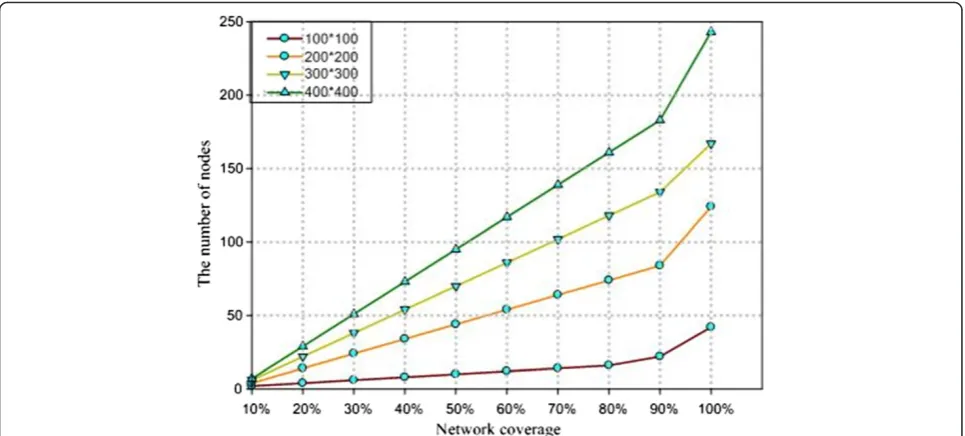
region. The model performance in different scales can be evaluated better. It is mainly reflected in the minimum number of nodes deployed in the cases of different coverage and network connectivity rate. The average value is derived from simulations of 100 times. The curve for node coverage variation in different network scales is shown in Figure 5.

As can be seen in Figure 5, firstly, there are less nodes for complete coverage in the network with smaller area and more nodes in larger area. For example, when cover-age is 100%, 43 nodes are needed in 100 * 100 area, 124 nodes in 200 * 200 area, 167 nodes in 300 * 300 area, and 243 nodes in 400 * 400 area. Secondly, the number of sensor nodes is not the same according to different requirements of networks for coverage rate. The number of nodes is increasing as the network grows, which shows a linear increasing relationship. In Figure 5, it requires more nodes to realize the full coverage for much larger networks and fewer nodes for smaller networks. When the coverage rate is between 90% and 100%, the increment rate of large network increases faster than that of the small-scale networks.

To further verify the coverage rate of WSN in probability model, the 100 * 100 model is chosen for study. After the network parameters are given dynam-ically, the proportion between network coverage rate and the number of nodes is compared, as shown in Figure 6.

Figure 6 shows the network coverage rate under different parameters; its computation process is according to formula (20), when stochastic variable follows normal distribution N∼(μ, σ2), p(X≤b) =ϕ((b−μ)/σ) is used

(14)

to get the result. Takeμ= 10,σ= 15 as an example, when the coverage rate is 60%, p(X≤b) =ϕ((b−10)/15)≥60%, it can be deducted that ((b−10)/15) = 0.255, and b =

⌈13.825⌉= 14. μ= 10, σ= 15, when the coverage rate is 60%, the required number of nodes is 14. From Figure 6, we can also see that, in case of same network size, the lar-ger the expectation, the more nodes will be required, i. e., the normal distribution model that the network shows. For any curve, the variation is a linear relation-ship that is because at first, the coverage rate increases at 5%, so the distributed function values changes slowly.

Second, the difference of expectation in the example is 10, which means the two adjacent curves have the feature of equal spacing. Third, when the coverage rate exceeds 95%, the number of nodes increased significantly. That is due to the quick change of distributed function values between 95% and 99.9%. For example, if the ex-pectation is 10 and variance is 15, 35 nodes are needed with coverage rate 95% while 55 is needed with coverage rate 99.9%.

For another important factor of WSN connectivity, the size of connectivity is directly related to the performance Figure 6Curve for network coverage variation with different parameters.

(15)

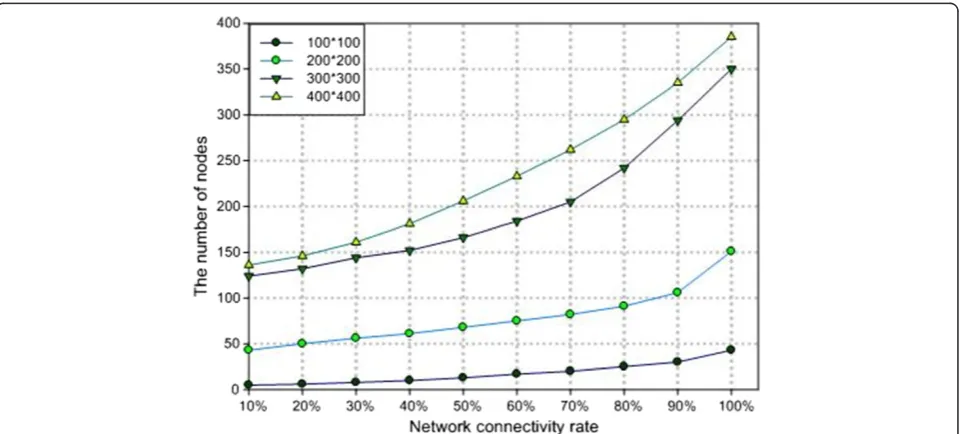
of data transmission, data processing, data computation, etc. Next, four different network models are adopted to compare the connectivity of WSN in experiments. Accord-ing to formulas (21), (22), and (23), the number of sensor nodes in different network models are solved, as is shown in Figure 7.

Figure 7 reflects the variation curves between network connectivity rate and the number of nodes. For the two networks of 100 * 100 and 200 * 200, the number of nodes increases more slowly. The main reasons are. first, when the network is small and the connectivity rate is 100%, 48 nodes can complete the connectivity between

nodes in the network model of 100 * 100 while 150 nodes are needed in the network model of 200 * 200. Second, for the two network models, the increasing trends of the node number are relatively stable. The node number increments is in linear relationship with time. For the two networks of 300 * 300 and 400 * 400, because their areas are larger, more nodes are needed compared with the previous two network models. At the beginning, the node number in the two network models is almost the same. However, with the expansion of the network model, the nodes are greatly increasing in 400 * 400 network model because in the communication process, the optimal communication Figure 8The relationship between number of sensor nodes and network energy.

(16)

rule is that the two circles of sensor nodes are circum-scribed, which is, however, impossible to achieve. There-fore, as the network grows, much more nodes are largely required.

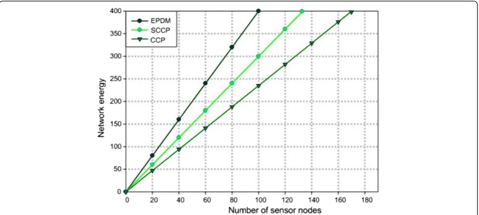
Figures 8 and 9 show the comparison between network energy and node number along with the rest energy of nodes changing with time for the event probability driven mechanism (EPDM) algorithm and algorithms of CCP and square region-based coverage and connectivity prob-ability model (SCCP) with the precondition of network coverage. As can be seen from the figure, with the same node number, the progressively increased speed of EPDM algorithm is larger than that of the algorithms of CCP and SCCP. For a certain energy value, the nodes of EPDM algorithm are much less than that of the other two algo-rithms. Figure 9 reflects that the total remaining energy of network nodes is decreased gradually with time in the operation of system. Compared with the other two algo-rithms, less energy is consumed while the network coverage can be ensured through this algorithm. After the network runs for the same period of time, 9% energy in average can be saved by using this algorithm than SCCP and 17% energy than CCP. This is because it costs little in the calculation of network coverage and less energy of sensor nodes is consumed.

6 Conclusions

This paper researches the coverage algorithm in wireless sensor networks and presents EPDM algorithm with the theory of probability. First, EPDM establishes the relation model and association relation between sensor nodes and target nodes. Then, the calculation of a target node's trajectory is given based on its probability and expectation. Next, target nodes can be covered more effectively through scheduling mechanism of nodes. The simula-tion results show that EPDM is effective and scalable. In future research, EPDM will be extended to implement the multiple coverage in heterogeneous wireless sensor network. Furthermore, we will study how to do quadratic linear programming for nodes with random distribution and improve the calculating precision for the border coverage.

Competing interests

The authors declare that they have no competing interests.

Acknowledgements

The authors would like to thank the National‘863’High Technology Research and Development Plans for funding projects under Grant Nos. 2011A01A204 and 2012A A01A306, the National Natural Science Foundation of China under Grant Nos.61170245, Science of Technology Research of Foundation Project of Henan Province Education Department under Grant Nos. 2014B520099, Natural Science Foundation for Young Scientists of Shanxi Province under Grant Nos. 2013JQ8024, and Natural Science and Technology Research of Foundation Project of Henan Province Department of Science under Grant Nos. 142102210471.

Author details

1

School of Electronics and Information Engineering, Xi’an Jiaotong University, Xi’an, Shaanxi Province 710049, China.2_{Department of Computer and} Information Engineering, Luoyang Institute of Science Technology, Luoyang, Henan Province 471023, China.3_{School of Computer Science and Education} Software, Guangzhou University, Guangzhou, Guangdong Province 510006, China.

Received: 7 November 2013 Accepted: 31 March 2014 Published: 14 April 2014

References

1. C Schuragers, V Tsiatsis, S Ganeriwal, M Srivastava, Optimizing sensor networks in the energy-latency-density design space. IEEE Trans. Mobile Comput.1(1), 70–80 (2002)

2. T Hou, Y Shi, HD Sherali, Rate allocation and network lifetime problems for WSN. IEEE/ACM Trans. Networking16(2), 321–334 (2008)

3. S He, J Chen, Y Sun, Coverage and connectivity in duty-cycled WSNs for event monitoring. IEEE Trans. Parallel Distr Syst23(3), 75–482 (2012) 4. K Derr, M Manic, WSN configuration-part II: adaptive coverage for decentralized

algorithms. IEEE Trans. Industrial Informatics9(3), 1728–1738 (2012) 5. W Li, W Zhang, Coverage analysis and active scheme of WSNs. Inst. Eng.

Technol.2(2), 86–91 (2012)

6. K Lin, JJPC Rodrigues, G Hongwei, N Xiong, X Liang, Energy efficiency QoS assurance routing in WSN. IEEE Syst. J.5(4), 495–505 (2011)

7. R Zhu, Y Qin, C-F Lai, Adaptive packet scheduling scheme to support real-time traffic in WLAN mesh networks. KSII Trans. Internet Inf. Syst.

5(9), 1492–1512 (2011)

8. S-T Cheng, J-S Shih, T-Y Chang, G-T Horng, C-T Chou, MLPA-conservation mechanism in WSN environments. EURASIP J. Wirel. Commun. Netw.

1, 1–13 (2012)

9. HR Karkvandi, E Recht, O Yadid Pecht, Effective lifetime-aware routing in WSNs. IEEE Sensors J.11(12), 3359–3367 (2011)

10. S Zairi, B Zouari, E Niel, E Dumitrescu, Nodes self-scheduling approach for maximizing WSN lifetime based on remaining energy. The Institution of. Eng. Technol.2(1), 52–62 (2012)

11. R Zhu, Intelligent rate control for supporting real-time traffic in WLAN mesh networks. J. Netw. Comput. Appl.34(5), 1449–1458 (2011)

12. C-f Hsin, M Liu, Randomly duty-cycled WSNs: dynamics of coverage. IEEE Trans. Wireless Commun.5(11), 3182–3892 (2006)

13. B Wang, K Chaning, W Wang, Information coverage in randomly deployed WSN. IEEE Trans. Wireless. Communications6(8), 2994–3004 (2007) 14. Y Xiao, H Chen, K Wu, B Sun, Y Zhang, X Sun, C Liu, Coverage and

detection of a randomized scheduling algorithm in WSNs. IEEE Trans. Comput.59(4), 507–521 (2010)

15. J-W Lin, Y-T Chen, Improving the coverage of randomized scheduling in WSN. IEEE Trans. Wireless Commun.7(2), 4807–4812 (2008)

16. S Slijepcevic, M Potkonjak, Power Efficient Organization of WSN, in

Proceedings of IEEE International Conference on Communications(Helsinki Finland, 2001), pp. 472–476

17. P Berman, G Calinescu, C Shah, A Zelikovsky, Power efficient monitoring management in sensor networks, inProceeding of IEEE Wireless Communication and Networking Conference(Atlanta, USA, 2004), pp. 2329–2334

18. D Tian, ND Georganas, A node scheduling scheme for energy conservation in large WSNs. Wirel. Commun. Mob. Comput.3(2), 271–290 (2003) 19. Z Abrams, A Goel, S Plotkin, Set K-cover algorithms for energy efficient

monitoring in WSN, inProceeding of the 3thInternational Symposium on Information Processing in Sensor Networks(Berkeley, California, USA, 2004), pp. 424–432

20. H Zhang, CH Jennifer, Maintaining sensing coverage and connectivity in large sensor network. Ad Hoc Sensor Wireless Netw.1(2), 89–124 (2005) 21. CF Huang, YC Tseng, The Coverage problem in a WSN, inProceeding of the

2nd ACM International Workshop on WSNs and Applications(San Diego, California, USA, 2003), pp. 115–121

22. M Cardei, DZ Du, Improving WSN lifetime through power aware organization. Wirel. Netw11(3), 333–340 (2005)

23. H Liu, P Wan, CW Yi, X Jia, SAM Makki, N Pissinou, Maximal lifetime scheduling in sensor surveillance networks, inProceedings of the 24th

(17)

24. J Wu, F Dai, M Gao, I Stojmenovic, On Calculating power-aware connected dominating sets for efficient routing in Ad Hoc Wireless network. J. Commun. Netw.4(1), 1–12 (2002)

25. K Kar, S Banerjee, Node placement for connected coverage in sensor networks, inProceedings of the Modeling and Optimization in Mobile, Ad Hoc and Wireless Networks(Sophia-Antipolis, France, 2003)

26. X Xing, G Wang, J Wu, J Li, Square region-based coverage and connectivity probability model in WSNs, inMobile Ad-Hoc and Sensor Networks (MSN), 2010 sixth International Conference(Hang Zhou, China, 2010), pp. 79–84 27. Y Li, C Vu, C Ai, G Chen, Y Zhao, Transforming complete coverage

algorithms to partial coverage algorithms for WSNs. IEEE Trans. Parallel Distrib. Syst.22(4), 695–703 (2011)

28. W Shu, J Wang, An optimized multi-hop routing algorithm based on clonal selection strategy for energy-efficient management in wireless sensor networks. Sensors and Transducers22(6), 8–14 (2013)

29. W Fang, F Liu, F Yang, L Shu, S Nishio, Energy-efficient cooperative communication for data transmission in WSN. IEEE Trans. Consum. Electron.56(3), 2185–2192 (2010)

doi:10.1186/1687-1499-2014-58

Cite this article as:Sunet al.:A novel coverage algorithm based on event-probability-driven mechanism in wireless sensor network.EURASIP Journal on Wireless Communications and Networking20142014:58.