ABSTRACT
RACE, SHAINA L. Iterative Consensus Clustering. (Under the direction of Carl Meyer.)
Iterative Consensus Clustering
by Shaina L. Race
A dissertation submitted to the Graduate Faculty of North Carolina State University
in partial fulfillment of the requirements for the Degree of
Doctor of Philosophy
Operations Research
Raleigh, North Carolina 2014
APPROVED BY:
Rada Chirkova William Stewart
Negash Medhin Carl Meyer
DEDICATION
ACKNOWLEDGEMENTS
TABLE OF CONTENTS
LIST OF TABLES . . . vii
LIST OF FIGURES . . . ix
Chapter 1 Introduction . . . 1
1.1 Clustering . . . 1
1.2 Data Clustering . . . 2
1.2.1 Mathematical Notation and Preliminaries . . . 2
1.2.2 Data . . . 3
1.2.3 Text Data . . . 5
1.2.4 The Number of Clusters,k . . . 5
1.3 Partitioning of Graphs and Networks . . . 6
1.4 History of Data Clustering . . . 9
Chapter 2 Algorithms for Data Clustering . . . 11
2.1 Hierarchical Algorithms . . . 11
2.1.1 Agglomerative Hierarchical Clustering . . . 11
2.1.2 Principal Direction Divisive Partitioning (PDDP) . . . 13
2.2 Iterative Partitional Algorithms . . . 16
2.2.1 Early Partitional Algorithms . . . 17
2.2.2 k-means . . . 19
2.2.3 k-mediods: Partitioning around Mediods (PAM) and Clustering Large Applications (CLARA) . . . 20
2.2.4 The Expectation-Maximization (EM) Clustering Algorithm . . . 21
2.3 Density Search Algorithms . . . 22
2.3.1 Density Based Spacial Clustering of Applications with Noise (DBSCAN) 23 2.4 Conclusion . . . 25
Chapter 3 Algorithms for Graph Partitioning . . . 27
3.1 Spectral Clustering . . . 27
3.1.1 Fiedler Partitioning . . . 28
3.1.2 Other Graph Cuts . . . 31
3.1.3 Power Iteration Clustering . . . 35
3.1.4 Clustering via Modularity Maximization . . . 36
3.2 Stochastic Clustering . . . 41
3.2.1 Stochastic Clustering Algorithm (SCA) . . . 41
Chapter 4 Dimension Reduction . . . 44
4.1 The Curse of Dimensionality . . . 44
4.1.1 Volume . . . 44
4.1.2 Distance and Similarity . . . 46
4.2 Dimension Reduction . . . 49
4.2.2 Principal Components Analysis (PCA) . . . 52
4.2.3 Alternative SVD Centerings . . . 54
4.2.4 Nonnegative Matrix Factorization . . . 55
4.2.5 Other Methods . . . 56
Chapter 5 Cluster Validation: Measuring the Quality of a Clustering . . . 58
5.1 Internal Validity Metrics . . . 59
5.1.1 General Cluster Cohesion and Separation: Graphs vs. Data . . . 59
5.1.2 Common Measures of Cohesion and Separation . . . 61
5.2 External Validity Metrics . . . 64
5.2.1 Accuracy . . . 64
5.2.2 Entropy . . . 66
5.2.3 Purity . . . 68
5.2.4 Mutual Information (MI) and Normalized Mutual Information (NMI) . 69 5.2.5 Other External Measures of Validity . . . 70
Chapter 6 Determining the Number of Clusters k . . . 74
6.1 Methods based on Cluster Validity (Stopping Rules) . . . 74
6.1.1 Sum Squared Error (SSE) Cohesion Plots . . . 75
6.1.2 Cosine-Cohesion Plots for Text Data . . . 76
6.1.3 Ray and Turi’s Method . . . 78
6.1.4 The Gap Statistic . . . 82
6.2 Graph Methods Based on Eigenvalues (Perron Cluster Analysis) . . . 85
Chapter 7 Consensus Clustering. . . 91
7.1 Consensus Clustering . . . 92
7.1.1 Benefits of the Consensus Matrix . . . 94
7.2 Previous Proposals for Consensus Clustering . . . 95
7.3 Iterative Consensus Clustering (ICC) . . . 96
7.3.1 The drop tolerance parameterτ . . . 100
7.4 Determining the Number of Clusters via Consensus Clustering . . . 101
7.4.1 Refining the Consensus Matrix through Iteration . . . 103
7.5 Conclusions . . . 104
Chapter 8 Results and Discussion . . . 106
8.1 Perron Cluster Analysis with Consensus Matrices . . . 106
8.1.1 AGBLOG Dataset . . . 106
8.1.2 Pendigits17 Dataset . . . 107
8.2 Comprehensive Cluster Analysis using Iterative Consensus Clustering . . . 109
8.2.1 Wine Dataset . . . 109
8.2.2 Newsgroups 6 Collection (NG6) . . . 115
8.3 Reaching Consensus . . . 121
8.3.1 Medlars-Cranfield-CISI (MCC) . . . 122
Chapter 9 Conclusions . . . 129
9.1 Contributions . . . 130
9.1.1 Determining the Number of Clusters . . . 130
9.1.2 The Consensus Matrix . . . 130
9.1.3 Iterated Consensus Clustering . . . 131
9.1.4 Dimension Reduction via NMF . . . 131
9.1.5 The Agreement Metric . . . 131
9.2 Future Work . . . 132
LIST OF TABLES
Table 5.1 Some Common External and Relative Indices . . . 71
Table 5.2 Some Common Measures of Overall Cohesion and Separation [49, 98] . . . . 73
Table 6.1 Approximated Number of Clusters via Ray and Turi’s Method . . . 81
Table 7.1 Accuracies of 7 Different Clustering Algorithms on 3 Subsets of Documents from the Same Corpus . . . 92
Table 7.2 Accuracy of 4 Algorithms on Raw Iris Data . . . 99
Table 7.3 Pairwise Agreement Between Algorithms on Raw Data . . . 99
Table 7.4 Accuracy of 4 Algorithms on Consensus Matrix 1 . . . 99
Table 7.5 Accuracy of 4 Algorithms on Consensus Matrix 2 . . . 100
Table 8.1 WINE Data: Summary of Results for Determining the Number of Clusters . . 114
Table 8.2 Dataset WINE: Accuracies for individual algorithms on raw data and con-sensus similarity matrices. . . 114
Table 8.3 Dataset WINE: Accuracies for spectral algorithms on different similarity ma-trices. . . 115
Table 8.4 Dataset WINE: 6 of 8 algorithms find a common solution in one iteration of the final consensus process . . . 115
Table 8.5 Dataset NG6: Accuracies for individual algorithms on raw data and dimen-sion reductions. . . 120
Table 8.6 Dataset NG6: Accuracies for individual algorithms on 3 different consensus matrices. . . 121
Table 8.7 Dataset NG6: Accuracies for spectral algorithms on different similarity ma-trices. . . 121
Table 8.8 Dataset NG6: 4 of 7 algorithms find a common solution in one iteration of the final consensus process . . . 121
Table 8.9 Accuracy Results for 3 Clustering Algorithms on 9 Low Dimensional Repre-sentations of the Medlars-Cranfield-CISI text data . . . 122
Table 8.10 Medlars-Cranfield-CISI text collection: Accuracies for 4 Clustering Algo-rithms on Consensus Matrices through Iteration . . . 123
Table 8.11 Dataset BenchmarkDFJX: Accuracy results for raw data and dimension re-ductions . . . 126
Table 8.12 Dataset BenchmarkDFJX: Accuracy results for consensus matrices through iteration . . . 126
Table 8.14 Dataset BenchmarkBCFG: Accuracy statistics for 100 trials ofk-means algo-rithm on consensus matrix . . . 127 Table 8.15 Dataset BenchmarkGHI: Accuracy results for raw data and dimension
re-ductions . . . 127 Table 8.16 Dataset BenchmarkGHI: Accuracy results for consensus matrices through
iteration . . . 128
LIST OF FIGURES
Figure 1.1 Three Meaningful Clusterings of One Set of Objects . . . 2
Figure 1.2 How Many Clusters doYouSee? . . . 6
Figure 1.3 A Graph with Clusters and its Block Diagonally Dominant Adjacency Matrix 7 Figure 1.4 Heat Map of Similarity Matrix Exhibiting Cluster Structure . . . 8
Figure 1.5 Matrix Heat Map Visualization from 1963 Book by Sokal and Sneath . . . 10
Figure 2.1 A Dendrogram exhibiting linkage/similarity between 9 objects in 3 clusters. 12 Figure 2.2 Illustration of Principal Direction Divisive Partitioning . . . 15
Figure 2.3 Failures of Principal Direction Divisive Partitioning . . . 16
Figure 2.4 Jancey’s method of reflecting old seed point across the centroid to deter-mine new seed point. . . 18
Figure 2.5 DBSCAN Illustration . . . 24
Figure 3.1 Fiedler Partitions and Zero Valuated Vertices . . . 30
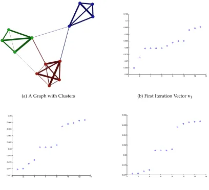
Figure 3.2 Power Iteration Clustering (PIC) Illustrated . . . 37
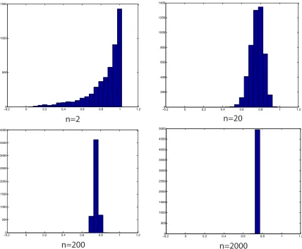
Figure 4.1 Distribution ofcdij for 100 random points inn-space . . . 47
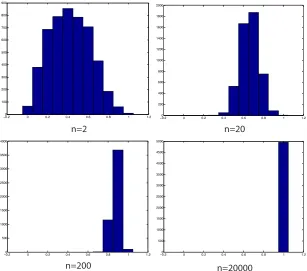
Figure 4.2 Distribution of cos(xi,xj)for 100 random points inn-space . . . 48
Figure 4.3 NMF Feature Extraction Illustrated . . . 56
Figure 5.1 The Difference between Cluster Cohesion Measures in Graph Partitioning vs. Data Clustering . . . 59
Figure 5.2 An Example of a Confusion Matrix . . . 64
Figure 5.3 A MoreConfusingConfusion Matrix . . . 65
Figure 5.4 Matching Predicted Class Labels to Actual Class Labels . . . 65
Figure 6.1 The Two-Dimensional Ruspini Dataset . . . 75
Figure 6.2 5 “Good” k-means Clusterings of the Ruspini Dataset and Corresponding SSE Plot . . . 77
Figure 6.3 Example of “Poor” Clusterings’ Effect on SSE Plot . . . 78
Figure 6.4 Sphericalk-means Objective Function Values for 2≤k≤20 . . . 79
Figure 6.5 SSE Plots for Medlars-Cranfield-CISI Clusterings using SVD Reduction tor dimensions . . . 80
Figure 6.6 Ray and Turi Validity Plot for Ruspini Data . . . 81
Figure 6.7 Ray & Turi’s Validity Plots for Medlars-Cranfield-CISI Clusterings on Raw Data and SVD Reductions tor dimensions . . . 82
Figure 6.9 Some Examples of Perron Cluster Identification . . . 90
Figure 7.1 Example of an Ensemble ofN =3 Clusterings . . . 93
Figure 7.2 The Consensus Matrix for the Ensemble in Figure 7.1 . . . 94
Figure 7.3 Distribution of Similarity Values in Cosine vs. Consensus Matrix . . . 95
Figure 7.4 Iterated Consensus Clustering (ICC) Process . . . 97
Figure 7.5 Iris Data (red = setosa, green = versicolor, blue = virginica) . . . 98
Figure 7.6 Dataset MCC: 20 Largest Eigenvalues Found Using Cosine Similarity Matrix 102 Figure 7.7 Dataset MCC: 20 largest eigenvalues found using consensus similarity ma-trices with (right) and without (left) the drop tolerance parameter τ. En-semble of 30 algorithms, each clustering data into ˜k=2, 3, . . . , 10 clusters . . 103
Figure 7.8 The Uncoupling Effect of Iteration: Matrix Heat Map . . . 104
Figure 7.9 The Uncoupling Effect of Iteration: Eigenvalues . . . 104
Figure 8.1 Dataset AGBLOG: Eigenvalues Associated with the Consensus Matrices Without (left) and With (right) a Drop Tolerance of τ=0.1 . . . 107
Figure 8.2 Dataset Pendigits17: Eigenvalues Associated with Traditional Similarity Ma-trices . . . 108
Figure 8.3 Dataset Pendigits17: Eigenvalues Associated with the Consensus Matrices of Two Different Cluster Ensembles . . . 109
Figure 8.4 Dataset WINE: SSE Plot . . . 111
Figure 8.5 Dataset WINE: Plots for the Gap Statistics . . . 111
Figure 8.6 Dataset WINE: Ray and Turi Plot (usingk-means clustering) . . . 112
Figure 8.7 Dataset WINE: Eigenvalues associated with consensus similarity matrices prior to iteration (right) and after iteration (left) using ˜k = 5, 6, 7, . . . , 10
clusters. The k∗ =3 eigenvalues in the Perron cluster correctly identify the number of clusters in both ensembles. . . 113
Figure 8.8 Dataset WINE: Eigenvalues from Gaussian Similarity . . . 113
Figure 8.9 Dataset NG6: SSE Plot for Sphericalk-means . . . 116
Figure 8.10 Dataset NG6: Ray and Turi Plot (Using Sphericalk-means ) . . . 117
Figure 8.11 Dataset NG6: Screeplot (First 100 Singular Values by Index) . . . 117
Figure 8.12 Dataset NG6: Eigenvalues associated with Initial (unadjusted) Consensus Matrix . . . 118
Figure 8.13 Dataset NG6: Eigenvalues associated with consensus similarity matrices ad-justed by drop tolerance (right) or adad-justed by iteration (left) using ˜k = 10, 11, 12, . . . , 20 clusters. The k∗ = 6 eigenvalues in the Perron cluster cor-rectly identify the number of clusters. . . 119
Figure 8.14 Dataset NG6: Eigenvalues associated with Cosine Similarity Matrix . . . 119
Figure 8.15 Dataset NG6: SSE Plot formed using the Consensus Matrix . . . 120
Chapter
1
Introduction
The purpose of this dissertation is to address two major problems that arise in applied cluster analysis: determining the number of clusters and determining a final solution from multiple algorithms. For years researchers have been innovating novel methods for cluster analysis. The vast majority of these algorithms require the user to specify the number of clusters for the algorithm to create. In an applied setting, it is unlikely that the user will know this information before hand. In fact, the number of distinct groups in the data may be the very question that an analyst is attempting to answer. Determining the number of clusters in data has long been considered one of the more difficult aspects of cluster analysis. This fact boils down to basics: what is a cluster? How do we define what should and should not count as two separate clusters? Our approach provides an original answer to this question: A group of points should be considered a cluster when a variety of algorithmsagreethat they should be considered a cluster. If a majority of algorithms can more or less agree on how to break a dataset into two clusters, but cannot agree on how to partition the data into more than two clusters, then we determine the data has two clusters. This is the essence of our approach.
An additional dilemma arises from the well accepted fact that no method is superior to all others for any type of real data. When many tools exist from which a user may choose, but no hard and fast guidelines are in place for making the choice of one particular tool over another, there is a problem. We propose a method which allows the user to use many of these tools at once, increasing his or her confidence in the final solution.
Before delving into the details of the proposed method, it will be necessary to cover all of the basics of cluster analysis. We start with a preliminary introduction to the field in this chapter.
1.1
Clustering
Figure 1.1. Here we have eight objects that differ by shape and color. Depending on the notion of similarity used (color, shape, or both) these objects might be clustered in one of the three ways shown.
Shape
Color
Shape & Color
Figure 1.1: Three Meaningful Clusterings of One Set of Objects
1.2
Data Clustering
In order to define this problem in a mathematical sense, it is necessary to quantify the at-tributes of objects using data so that we can mathematically or statistically determine notions of similarity. Data clustering, or cluster analysis, is one of the building blocks of modern data analysis. Data clustering refers to the process of grouping data pointsnaturallybased on in-formation found in the data which describes its characteristics and relationships. It is not an exact science and, as we will discuss at length later in Chapter 2, there is nobestmethod for partitioning data into clusters. First we discuss some notation and preliminaries.
1.2.1 Mathematical Notation and Preliminaries
Throughout this dissertation, we will stick to some common notational traditions. We list them here for your convenience:
• Capitalized, bold-faced letters (X,S,Petc.) will represent matrices.
• Lower-case bold-faced letters (x,u,v) will represent vectors.
• Subscripts on vectors indicate their column index inside a matrix (X= [x1, . . . ,xn]). • Double matrix subscripts or parenthetical arguments on a vector will be used to
• All vectors are assumed to be columns, thusxT will always represent a row vector.
• The vector of all ones will be represented ase.
• k ∗ kwill imply the Euclidean norm (2-norm) unless explicitly stated otherwise. • For a setS, |S| is the cardinality or number of elements contained inS.
We will also make use of the Singular Value Decomposition (SVD). While many of the pertinent properties of this matrix factorization are given in detail throughout this paper, some familiarity is implied. The SVD is formalized in Definition 1 and a few useful proper-ties are given here. For a more complete treatment of this important mathematical tool, we suggest for example [87, 52].
Definition 1(Singular Value Decomposition). For eachA∈Rm×nof rank r, there are orthogonal matricesUm×m,Vn×n, and a diagonal matrixDr×r=diag(σ1,σ2, . . . ,σr)such that
A=U D 0 0 0
!
m×n
VT withσ1≥ σ2≥ · · · ≥σr >0.
Theσi’s are called the nonzero singular valuesofA. This factorization is called the singular value decomposition of Aand the columns of U andV are called the left-hand and right-handsingular vectorsforA, respectively [87].
Some Important Properties of the SVD[87]
1. The first singular value is equal to the matrix two-norm:
σ1= max
kxk=1kAxk2=kAk2
2. The Frobenius norm of the matrix is also given by the singular values:
kAkF=
s
r
∑
i=1 σi2
3. Singular values represent distances to lower rank matrices:
σk+1 = min
rank(B)=kkA−Bk2
1.2.2 Data
Each data point will be considered as a column vector, containing measurements of features, attributes, or variables (again, used interchangeably) which characterize it. For example, a column vector characterizing a document could have as many rows as there are words in the dictionary, and each entry in the vector could indicate the number of times each word occurred in the document. An Iris flower, on the other hand, may be characterized by far fewer attributes, perhaps measurements on the size of its petal and sepal. It is assumed we haven such objects, each represented by a column vectorxj containing measurements onm variables. All of this information is collected in anm×n data matrix,X, which will serve as
input to the various clustering methods.
X= [x1,x2, . . . ,xn]
The aim of data clustering is to automatically determine clusters in these populations based upon the information contained in those vectors. In the document collection, the goal may be to identify clusters of documents which discuss similar subject matter whereas in the Iris population, the goal may be to identify the different species of Iris flowers.
In applied data mining, variables fall into the following four categories: Nominal/Categorical, Ordinal, Interval, or Ratio.
1. Nominal/Categorical:Variables which have no ordering, for example ethnicity, color or
shape.
2. Ordinal:Variables which can be rank-ordered but for which distances have no meaning.
For example, scores assigned to levels education (0=no high school, 1=some high school, 2=high school diploma). The distance between 0 and 1 is not necessarily the same as the distance between 1 and 2, but the numbers have some meaning by order.
3. Interval:Variables for which differences can be interpreted but for with ratios make no
sense. For example if temperature is measured in degrees Fahrenheit the distance from 20 to 30 degrees is the same as the distance from 70 to 80 degrees, however 80 degrees is not “twice as hot” as 40 degrees.
4. Ratio:variables for which a meaningful ratio can be constructed. For example height or
weight. An absolute zero is meaningful for a ratio variable.
1.2.3 Text Data
For this application, the objects to be clustered are called documents. The word document in this context refers to any piece of text - it could be a sentence, a paragraph, a webpage, or an entire article or book. Text is transformed into numerical data by means of a term-document matrix.Since a large number of our experiments involve text data, we formalize this structure in Definition 2.
Definition 2 (Term-Document Matrix). Let n be the number of documents in a collection and m be the number of terms appearing in that collection, then we create our term-document matrix Xas follows:
Doc 1 Doc j Doc n
Xm×n=
Term 1 Term i Term m | | | − − fij
where fi,j is the frequency of term i in document j.
Term-document matrices tend to be large and sparse. Term-weighting schemes are often used to downplay the effect of commonly used words and bolster the effect of rare but semantically important words [110, 10]. For the experiments contained herein, the popular “Term Frequency-Inverse Document Frequency” (TF-IDF) weighting method is employed. For this method, the raw term-frequencies fijin the matrixXare multiplied by global weights (inverse document frequencies),wi, for each term. These weights reflect the commonality of each term across the entire collection. Let D represent the entire document collection, dj represent the document jandti represent term i. The inverse document frequency of termi is:
wi =log
n
|{dj ∈ D :ti ∈dj}| .
To put this weight in perspective for a collection ofn=10, 000 documents we have 0≤wi ≤ 9.2. The document vectors are also normalized to have unit 2-norm, since their directions (not their lengths) in the term-space is what characterizes them semantically.
For the majority of text datasets contained herein, the term-document matrices were formed using the Text to Matrix Generator (TMG) for MATLAB. This tool was created by Dimitrios Zeimpekis and Efstratios Gallopoulos at The University of Patras in Greece [135].
1.2.4 The Number of Clusters, k
2-dimensional scatter plot of points in Figure 1.2. Using the points’ proximity in Euclidean space as a measure of their similarity, one could argue that there are any number of clusters in this simple illustration. However, most people would agree that there is indeed cluster-like structure in this data.
Figure 1.2: How Many Clusters doYouSee?
It is easy to imagine data in which the number of clusters to specify is a matter of de-bate only because groups of related objects can be meaningfully divided into subcategories orsubclusters.For example a collection of webpages may clearly fall into 3 categories: sports, investment banking, and astronomy. If the webpages about sports further divide into 2 cate-gories like baseball and basketball then we’d refer to that as subclustering. One of the aims of the method in Chapter 7 is to determine the most reasonable number of clusters in data based upon whether or not a majority of clustering algorithms can agree upon how exactly to partition the data into that particular number of clusters. Chapter 6 provides a thorough examination of existing procedures for determining the number of clusters.
1.3
Partitioning of Graphs and Networks
partition-A
B
C
(a) Graph
A
A
A
A
B
C
ε
ε
ε
AB
BC AC
ε
ABε
ACε
BCA=
(b) Reordered Adjacency Matrix
Figure 1.3: A Graph with Clusters and its Block Diagonally Dominant Adjacency Matrix
ing (or network community detection) will rely on an adjacency matrix. Anadjacency matrix Afor an undirected graph is ann×nsymmetric matrix defined as follows:
Aij =
wij, if(i,j)∈E 0 otherwise
Figure 1.3a is an example of a graph exhibiting cluster or community structure. The weights of the edges are depicted by their thickness. It is expected that edges within the clus-ters occur more frequently and with higher weight than edges between the clusclus-ters. Thus, once the rows and columns of the matrix are reordered according to their cluster member-ship, we expect to see a matrix that isblock-diagonally dominant - that is, one in which values in square diagonal blocks are relatively large compared to those in the off-diagonal blocks. The notion of block-diagonal dominance will be formalized in Chapter 6.
In much of the literature on graph partitioning, it is suggested that the data clustering problem can be transformed into a graph partitioning problem by means of a similarity ma-trix [32, 124, 103, 39]. Asimilarity matrix Sis ann×nsymmetric matrix whereSij measures some notion of similarity between data pointsxi andxj. There are a wealth of metrics avail-able to gauge similarity or dissimilarity, see for example [49]. Common measures of similarity rely on Euclidean or angular distance measures. Two of the most popular similarity functions in the literature are the following:
• Gaussian Similarity:
Sij =exp(−k
• Cosine Similarity:
Sij =cos(xi,xj) =
xTi xj
kxikkxjk
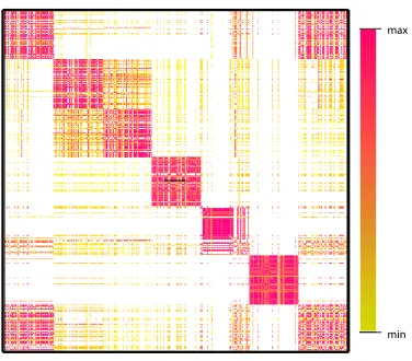
Any similarity matrix can be considered an adjacency matrix for a graph, thus trans-forming the original data clustering problem into a graph partitioning problem. Several al-gorithms for data clustering and graph partitioning are provided in Chapter 2. Regardless of the method chosen for clustering, similarity matrices can be a useful tool for visualizing cluster results in light of the block diagonal structure shown in Figure 1.3. This block diag-onal structure can be visualized using a heat map of a similarity matrix. A matrix heat map represents each value in a matrix by a colored pixel indicating the magnitude of the value. Figure 1.4 is an example of a heat map using real data. The data are a collection of news arti-cles (documents) from the web containing seven different topics of discussion. The rows and columns of the cosine similarity matrix for these documents have been reordered according to some cluster solution. White pixels represent negligible values of similarity. Some of these topics are closely related, which can be seen by the heightened level of similarities between blocks. This data collection, a subset of “twenty newsgroups”, will be revisited in Chapter 8.
max
min
Figure 1.4: Heat Map of Similarity Matrix Exhibiting Cluster Structure
analysis and how it emerged into a major field of research in the late twentieth century.
1.4
History of Data Clustering
According to Anil Jain in [60], data clustering first appeared in an article written by Forrest Clements in 1954 about anthropological data [25]. However, a Google Scholar search provides several earlier publications whose titles also contain the phrase “cluster analysis" [120, 2]. In fact, the discussion of data clustering dates back to the 1930’s when anthropologists Driver and Kroeber [35] and psychologists Zubin [136] and Tryon [1] realized the utility of such analysis in determining cultural or psychological classifications. While the usefulness of such techniques was clear to researchers in many social and biological disciplines at that time, the lack of computational tools made the analysis time consuming and practically impossible for large sets of data.
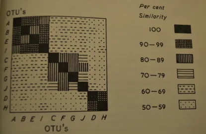
Cluster analysis exploded into the limelight in the 1960’s and ‘70’s after Sokal and Sneath’s 1963 bookPrinciples of Numerical Taxonomy[114]. Although the text is primarily geared toward biologists faced with the task of classifying organisms, it motivated researchers from many different disciplines to consider the problem of data clustering from other angles like com-puting, statistics, and domain specific applications. [13]. Sokal and Sneath’s book presents a detailed discussion of the simple, intuitive, and still popular hierarchical clustering (see Sec-tion 2.1) techniques for biological taxonomy. These authors also provided perhaps the earliest mention of the matrix heat map visualizations of clustering that are still popular today. Fig-ure 1.5 shows an example of one of these heat maps, then drawn by hand, from their book.
Chapter
2
Algorithms for Data Clustering
There have been countless algorithms proposed for data clustering. While a complete survey and discussion of clustering algorithms would be nearly impossible, this chapter provides an introduction to some of the most popular algorithms to date. For the purposes of or-ganization, the algorithms are divided into 3 groups: Hierarchical, Iterative Partitional, and Density-based.
2.1
Hierarchical Algorithms
As discussed in Chapter 1, data clustering became popular in the biological fields of phy-logeny and taxonomy. Even prior to the advancement of numerical taxonomy, it was common for scientists in this field to communicate relationships by way of adendrogramor tree diagram as illustrated in Figure 2.1 [114]. Dendrograms provide a nested hierarchy of similarity that allow the researcher to see different levels of clustering that may exist in data, particularly in phylogenic data.Agglomerative hierarchical clusteringhas its roots in this domain.
2.1.1 Agglomerative Hierarchical Clustering
highest branch of the dendrogram is cut, the result is two clusters: {{1,2,3},{4,5,6,7,8,9}}. When the next highest branch is cut, we are left with 3 clusters: {{1,2,3},{4,5,6},{7,8,9}}.
1 2 3 4 5 6 7 8 9
Figure 2.1: A Dendrogram exhibiting linkage/similarity between 9 objects in 3 clusters.
There are a number of different systems for determining linkage in hierarchical clustering dendrograms. For a complete discussion, we suggests the classic books by Anderberg [4] or Jain and Dubes [61]. The basic scheme for hierarchical clustering algorithms is outlined in Algorithm 1.
Algorithm 1Agglomerative Hierarchical Clustering Input: n objects to be clustered.
1. Begin by assigning each object to its own cluster.
2. Compute the pairwise similarities between each cluster.
3. Find the most similar pair of clusters and merge them into a single cluster. There is now one less cluster.
4. Compute pairwise similarities between the new cluster and each of the old clusters. 5. Repeat steps 3-4 until all objects belong to a single cluster of size n.
Output: Dendrogram depicting each merge step.
dissim-ilarity) between objects in step 2. In step 4, the same notion of similarity must be extended to compare clusters of objects. Several methods of computing pairwise distances between clusters have been proposed over the years. The most common approaches are as follows:
Single-Linkage
The distance between two clusters is equal to theshortestdistance from any member of one cluster to any member of the other cluster.
Complete-Linkage
The distance between two clusters is equal to thegreatestdistance from any member of one cluster to any member of the other cluster.
Average-Linkage
The distance between two clusters is equal to theaveragedistance from any member of one cluster to any member of the other cluster.
While many people have been given credit for the methods listed above, it appears that numerical taxonomers Sneath, Sokal and Michener were the first to describe the Single- and Average-linkage protocols, while ecologist Sorenson had previously pioneered Complete-linkage in his ecological studies. These early researchers used correlation coefficients to measure similarity between objects, but they suggest in 1963 that other correlation-like or distance-like measures could also be useful [114]. The paper by Stephen Johnson in 1967 [64] formalized the single- and complete-linkage algorithms in a more general data clustering setting. Other linkage techniques for hierarchical clustering, such as centroid and median linkage, have been proposed as well. We refer interested readers to Anderberg [4] for more on these variants.
The main drawback of agglomerative hierarchical schemes is their computational com-plexity. In recent years, variations like BIRCH [121] and CURE [54] have been developed in an effort to combat this problem. Another feature which causes problems in some applica-tions is that once a connection between points or clusters is made, it cannot be undone. For this reason, hierarchical algorithms often suffer in the presence of noise and outliers.
2.1.2 Principal Direction Divisive Partitioning (PDDP)
While the hierarchical algorithms discussed above were agglomerative, it is also possible to create a cluster hierarchy or dendrogram by iteratively dividing points into groups until a desired number of groups is reached. Principal Direction Divisive Partitioning (PDDP) is one example of adivisive hierarchical algorithm. Other partitional methods which will be discussed in Chapter 3 can also be placed in this hierarchical framework.
squares lineLis the line which minimizes the total sum of squares of orthogonal deviations between the data andLamong all lines inRm. LetX= [x
1,x2, . . . ,xn]be the data points and
L(u,p) be a line in Rm where p is a point on a line and u is the direction of the line. The projection ofxj ontoL(u,p)is given by
b
xj =uuT(xj−p) +p, and therefore the orthogonal distance betweenxj andL(u,p)is
xj−xbj = (I−uuT)(xj−p).
Consequently, the total least squares line is the lineLwhich minimizes (over directionsuand
pointsp)
f(u,p) =
n
∑
j=1
kxj−xbjk22
=
n
∑
j=1k
(I−uuT)(xj−p)k22
=k(I−uuT)(X−peT)k2F.
(2.1)
The following definition precisely characterizes the total least squares line.
Definition 3. Total Least Squares Line.
Thetotal least squares linefor the column data inX= [x1,x2, . . . ,xn]is given by
L={αu1(Xc) +µ|α∈R},
where µ = Xe/n is the mean (centroid) of the column data, and u1(Xc) is the principal left-hand singular vector of the centered matrix
Xc =X−µeT =X(I−eeT/n).
u1(Xc)is also known as thefirst principal componentofX.
The orthogonal projection of the data onto the total least squares line will capture the maximum amount of directional variance over all possible one dimensional orthogonal pro-jections. This fact is treated in greater detail in Chapter 4.
Boley’s PDDP algorithm partitions the data into two clusters at each step based upon whether their projections onto the total least squares line fall to the left or to the right ofµ.
αu (X )1 C
(a) Data with 2 clusters
v (i) <01 v (i) >01
(b) Data Projected onto Total Least Squares Line
Figure 2.2: Illustration of Principal Direction Divisive Partitioning
Once the data are divided, the two clusters are examined to find the one with the greatest variance (scatter). This subset of data is then extracted from the original data matrix, centered and projected onto the span of its own first principal component. The split at zero is made again and the algorithm proceeds iteratively until the desired number of clusters has been produced.
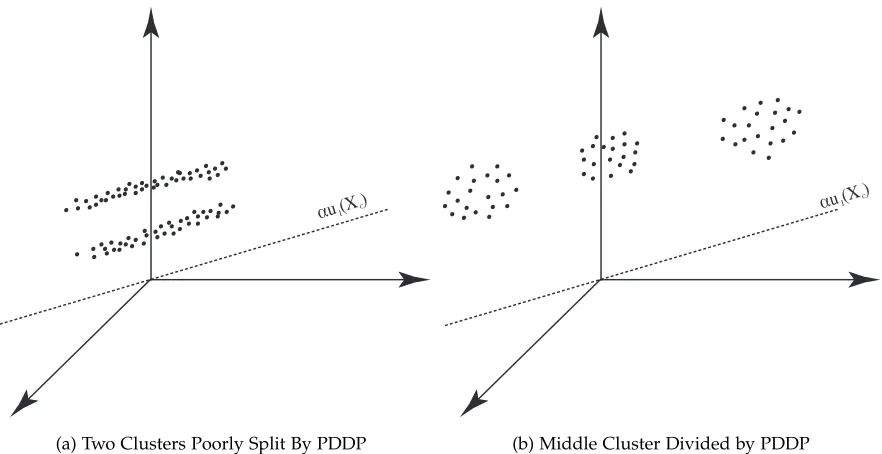
It is necessary to note, however, that the example in Figure 2.2 is truly an ideal geometric configuration of data. Figure 2.3 illustrates configurations in which PDDP would fail. In Figure 2.3a, both clusters would be split down the middle, and in Figure 2.3b the middle cluster would be split in the first iteration. Unfortunately, once data points are separated in an iteration of PDDP, there is no chance for them to be rejoined later. The steps of PDDP are given in Algorithm 2.
αu (X )1 C
(a) Two Clusters Poorly Split By PDDP
αu (X )1 C
(b) Middle Cluster Divided by PDDP
Figure 2.3: Failures of Principal Direction Divisive Partitioning
Algorithm 2Principal Direction Divisive Partitioning (PDDP)
Input:ndata pointsX= [x1,x2, . . . ,xn]and number of clustersk 1. Center the data to have mean zero:Xc =X−µeT.
2. Compute the first right singular vector ofXc,v1.
3. Partition the data into two clusters based upon the signs of the entries in v1.
4. Compute the variance of each existing cluster and choose the cluster with largest vari-ance to partition next.
5. Repeat steps 1-4 using only the data in the cluster with largest variance until eventually kclusters are formed.
Output:Resultingk-clusters
2.2
Iterative Partitional Algorithms
“better" partition [61, 4]. The k-means algorithm is one example of a partitional algorithm. Before we get into the details of the modern dayk-means algorithms, we’ll take a look back at the history that fostered its development as one of the best-known and most widely used clustering algorithms in the world.
2.2.1 Early Partitional Algorithms
Although the name “k-means " was first used by MacQueen in 1967 [78], the partitional method generally referred to by this name today was proposed by Forgy in 1965 [46]. Forgy’s algorithm involves iteratively updating k seed points which, at each pass of the algorithm, define a partitioning of the data by associating each data point with its nearest seed point. The seeds are then updated to represent the centroids (means) of the resulting clusters and the process is repeated. Euclidean distance is the most common metric for measuring the nearness of points in these algorithms, but other metrics, such as Mahalanobis distance and angular distance, can and have been used as well.K-means can also handle binary or categor-ical variables by using simple matching coefficients found in the data mining literature, for example [98]. Forgy’s method is outlined in Algorithm 3. In 1966, Jancey suggested a
varia-Algorithm 3Forgy’sk-means Algorithm [4]
Input: Data points and an initial cluster configuration of the data, defined by k seed points (start in step 1) or an initial clustering (start in step 2).
1. Assign each data point to the cluster associated with the nearest seed point. 2. Compute new seed points to be the centroids of the clusters.
3. Repeat steps 1 and 2 until no data points change cluster membership in step 2.
Output: Final Clusters
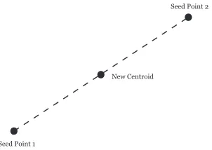
tion of this method where the new seeds points in step 2 were computed by reflecting the old seed point across the new centroid, as depicted in Figure 2.4. Jancey argued that the data’s nearness to point 1 grouped them into a cluster initially, and thus using a seed point which exaggerates this movement toward the new centroid ought to help speed up convergence, and possibly lead to a better solution by avoiding local minima [62].
Seed Point 1
New Centroid
Seed Point 2
Figure 2.4: Jancey’s method of reflecting old seed point across the centroid to determine new seed point.
Algorithm 4MacQueensk-means Algorithm Input:ndata points
1. Choose the first kdata points as clusters with one member each. Set i=1.
2. Assign the (k+i)th data point to the cluster with the closest centroid. Recompute the cetroid of the updated cluster. Seti=i+1.
3. Repeat step 2 untili=n−kand all the data points have been assigned. Use final cluster centroids to determine a final clustering by re-assigning each data point to the cluster associated with its nearest centroid.
Output: Final Clusters
2.2.2 k-means
We will finish our discussion of k-means with what has become the classical presentation. We begin with a matrix of column data, X = [x1,x2, . . . ,xn] where xi ∈ Rm, 1 ≤ i ≤ n. The objective ofk-means is to determine a partitioning of the data intoksets,C= {C1,C2, . . . ,Ck}, such that an intra-cluster sum of squares cost function is minimized:
arg min C
k
∑
i=1x
∑
j∈Cikxj−µik2
Any desired distance metric can be used, according to the applications and whims of the user. Euclidean distance is standard, and leads to the specificationEuclidean k-means. In document clustering, it is common to use the cosine of the angle between two data vectors (documents) to measure their distance from each other. This variant is commonly referred to as spheri-cal k-means and will be discussed briefly in Section 2.2.2. The k-means algorithm, which is essentially the same as Forgy’s algorithm in Section 2.2, is presented in Algorithm 5.
Algorithm 5Euclideank-means
Input: Data points{x1,x2, . . . ,xn}and set of initial centroids{µ1(0),µ(20), . . . ,µ(k0)}.
1. Assign each data point to cluster associated with the nearest centroid.
Cj(t) ={xi :kxi−µ(jt)k ≤ kxi−µ(lt)k ∀1≤l≤k}
If two centroids are equally close, the tie is broken arbitrarily. 2. The new centroid for each cluster is calculated by setting
µ(jt+1)= 1
|C(jt)|x
∑
i∈C(t)j
xi
3. Repeat steps 2 and 3 until the centroids remain stationary.
Output:k clustersC1,C2, . . . ,Ck
cost function at each step. However, it is quite common for the algorithm to converge to local minima, particularly with large datasets. The output ofk-means is sensitive to the initializa-tion of the centroids and the choice of distance metric used in step 2. Randomly initialized centroids tend to be the most popular, but one can also seed the algorithm with centroids of clusters determined by another clustering algorithm. We will implement both approaches for our experiments in Chapter 8. One of the objectives of our method in Chapter 7 is to combine results from multiple trials of the algorithm using different initializations.
Sphericalk-means
In some applications, such as document clustering, similarity is often measured by the cosine of the angleθ between two objectsxi andxj (each normalized to have unit norm),
cos(θ) =xTi xj.
This similarity is often transformed into a distance by computing the quantity d(xi,xj) = 1−cos(θ)to formulate the sphericalk-means objective function as follows:
min C
k
∑
i=1x
∑
∈Ci1−xTci.
Whereci = kµ1
ikµi is the normalized centroid of the cluster. The sphericalk-means algorithm
is the same as the euclideank-means algorithm aside from the definition of nearness in step 2.
2.2.3 k-mediods: Partitioning around Mediods (PAM) and Clustering Large Ap-plications (CLARA)
results in the lowest average distance is retained [67].
2.2.4 The Expectation-Maximization (EM) Clustering Algorithm
The Expectation-Maximization (EM) Algorithm, originally proposed by Dempster, Laird, and Rubin in 1977 [5], is one that has been used to solve many types of statistical problems over the years. It is generally used to determine parameters of a statistical model used to describe observations in a dataset. Here we will show how the algorithm is used for clustering, as in [22]. Our discussion is limited to the variant of the algorithm which uses Gaussian mixtures to model the data.
Supposing that our data points, x1,x2, . . . ,xn, each belonging to one of k clusters (or classes), C1,C2, . . . ,Ck. Then there exists some latent variables yi, 1 ≤ i ≤ n, which iden-tify the class membership of each xi. It is assumed that each class label Ci determines the probability distribution of the data in that class. Here, we assume that this distribution is multivariate Gaussian. The parameters of this model include the a priori probabilities of each of the kclasses, P(Ci), and the parameters of the corresponding normal distributionsµi and Σi, which are the mean and covariance matrix respectively. The objective of the EM algorithm is to determine the parameters which maximize the likelihood of the data:
logL =
∑
i
(logP(yi) +logP(xi|yi))
The EM algorithm takes as input a set of m-dimensional data points, {xi}ni=1, the desired
number of clusters k, and an initial set of parameters θj for each cluster Cj 1 ≤ j ≤ k. For Guassian mixtures, θj consists of mean µj and an m×m covariance matrix Σj. The a priori probability of each cluster, αj = P(Cj)must also be initialized and updated throughout the algorithm. If no information is known about the underlying clusters, then we suggest initial-ization αj = 1/k for all clusters Cj. EM then operates by iteratively executing an expectation step, where the probability that each data point belongs to each of thek classes is computed, followed by amaximization step, where the parameters for each class are updated to maximize the likelihood of the data [22]. These steps are summarized in Algorithm 6.
The EM Algorithm with Gaussian mixtures works well for clustering when the normality assumption of the underlying clusters holds true. Unfortunately, it is difficult to know if this is the case prior to the identification of the clusters. The algorithm suffers considerable computational drawbacks, particularly with regards to storage of the k covariance matrices
Algorithm 6Expectation-Maximization Algorithm for Clustering [22]
Input:ndata points,{xi}ni=1, number of clustersk, and initial set of parameters for each clusterCj:αj andθj ={µj,Σj} 1≤j≤k
1. Expectation Step: Compute the probability of each data pointxi being drawn from each class distribution,Cj:
pij = P(xi|αj,µj,Σj)∝αjP(xi|µj,Σj)
2. Maximization Step: Update the parameters to maximize the likelihood of the data:
αj = 1 n
n
∑
i=1 pij
µj = ∑
n i=1pijxi
∑n
i=1pij
Σj =
∑n
i=1pij(xi−µj)(xi−µj)T
∑n
i=1pij 3. Repeat steps 1-2 until convergence.
Output: Class label jfor eachxi such thatpij ≥ pil 1≤l≤k
2.3
Density Search Algorithms
If objects are depicted as data points in a metric space, then one may interpret the problem of clustering as an attempt to find areas of the space that are densely populated by points, sep-arated by less populated areas. A natural approach to the problem is then to search through the space seeking these dense regions. Such algorithms have been referred to asdensity search algorithms [38]. While these algorithms tend to suffer on real data in both accuracy efficiency, their ability to identify noise and to estimate the number of clusterskmakes them worthy of discussion.
cluster.
The conception of density search algorithms dates to the late ‘60s with thetaxmapmethod of Carmichael et al. in [21, 20] and themode analysis method of Wishart [128]. In taxmapthe authors suggested criterion like the drop in average similarity upon adding a new point to a cluster. Inmode analysis the criterion was simply containment in a specified radius of points in a cluster. The problem with this approach was that it had trouble finding both large and small clusters simultaneously [38].
All density search algorithms suffer from the inability to find clusters of varying density, no matter how the term is defined in application, because the density of points is used to define the notion of a cluster. High dimensional data adds to this problem as demonstrated in Chapter 4 because as the size of the space grows, the points naturally become less and less dense inside of it. Another problem with density search algorithm is the necessity to search through data again and again, making their implementation difficult if not irrelevant for large data sets. Among the benefits to these methods are the inherent estimation of the number of clusters and their ability to find irregularly shaped (non-convex) clusters. Several algorithms in this category, like Density Based Spacial Clustering of Applications with Noise (DBSCAN) also make an effort to determine outliers or noise in the data. Because of the computational workload of these methods, we will abandon them after the present discussion in favor of more efficient methods. For an in-depth analysis of other density search algorithms and their variants, see [23].
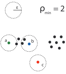
2.3.1 Density Based Spacial Clustering of Applications with Noise (DBSCAN) Density Based Spacial Clustering of Applications with Noise (DBSCAN) is an algorithm pro-posed by Ester, Kriegel, Sander, and Xu in 1996 [37], which uses the Euclidean nearness of a group of points inm-space to define density. The algorithm uses the following definitions and parameters to determine what constitutes a cluster:
Dense Point andρmin
A point xj is called dense if there are at least ρmin other points contained in its e -neighborhood.
Direct Density Reachability
A pointxi is calleddirectly density reachablefrom a pointxj if it is in thee-neighborhood surroundingxj, i.e. ifxi ∈N(xj,e),andxj is a dense point.
Density Reachability
A point xi is called density reachable from a point xj if there is a sequence of points
x1,x2, . . . ,xp with x1 = xj and xp = xi where each xk+1 is directly density reachable fromxk.
Noise Point
The relationship of density reachability is not symmetric. This fact is illustrated in Figure 2.5. A point in this illustration is dense if its e-neighborhood contains at least ρmin = 2 other points. The green point a is density reachable from the blue pointb, however the reverse is not true because a is not a dense point. Because of this, we introduce the notion of density connectedness.
ε
ρ
min
= 2
b
c a
Figure 2.5: DBSCAN Illustration
Density Connectedness
Two pointsxi andxj are density-connectedif there exists some point xk such that bothxi andxj are density reachable from xk.
In Figure 2.5, it is clear that we can say points a andb are density-connected since they are each density reachable from any of the 4 points in between them. The pointcin this illustra-tion is a noise point or outlier because there are no points contained in itse-neighborhood.
Using these definitions, we can formalize the properties that define a cluster in DBSCAN. Given the parameters ρmin and e, a cluster is a set of points that satisfy the two following conditions:
1. All points within the cluster are mutually density-connected.
Algorithm 7Density Based Spacial Clustering of Applications with Noise (DBSCAN) [98] Input:Set of pointsX= [x1,x2, . . . ,xn]to be clustered and parameterseandρmin
1. For each unvisited point p=xi, do: I. Mark pas visited.
II. LetN be the set of points contained in the e-neighborhood around p. (a) If|N |<ρminmark p as noise.
(b) Else let Cbe the next cluster. Do: i. Add pto clusterC.
ii. For each pointp0 inN, do:
A. If p0 is not visited, mark p0 as visited, let N 0 be the set of points
con-tained in thee-neighborhood around p0. If|N0| ≥ρmin letN =N ∪ N0 B. If p0 is not yet a member of any cluster, add p0 to clusterC.
Output:Clusters foundC1, . . . ,Ck
2.4
Conclusion
The purpose of this chapter was to give the reader a basic understanding of hierarchical, iter-ative partitional, and density search approaches to data clustering. One of the main concerns addressed in this paper is that all of these algorithms have merit, but in application rarely do the algorithms completely agree on a solution. In fact, algorithms with random inputs like k-means are not even likely to agree with themselves over a number of different trials. It can be extremely difficult to qualitatively measure the goodness of your clustering when the data cannot be visualized in 2 or 3 dimensions. While there are a number of metrics to help the user get a sense of the compactness of the clusters (see Chapter 5), the effect of noise and outliers can often blur the true picture. It is also common for such metrics to take nearly equivalent values for vastly different cluster solutions, forcing the user to choose a solution in an ad hoc manner. In Chapter 7 we will present a solution to this ambiguity by using multiple algorithms to obtain a solution with which the user can have more confidence. First we will look at another class of clustering methods which aim to solve the graph partitioning problem described in Chapter 1.
Chapter
3
Algorithms for Graph Partitioning
3.1
Spectral Clustering
Spectral clustering is a term that data-miners have given to the partitioning problem as it arose in graph theory. The theoretical framework for spectral clustering was laid in 1973 by Miroslav Fiedler [42, 43]. We will begin with a discussion of this early work, and then take a look at how others have adapted the framework to meet the needs of data clustering. In this setting, we have a graph G on a set of vertices N = {1, 2, . . . ,n}with edge set E = {(i,j) :
i,j∈ Nandi↔ j}. Edges between the vertices are recorded in anadjacency matrixA= (aij), where aij is equal to the weight of the edge connecting vertex (object) i and vertex j and aij =0 if(i,j)∈/ E.
A graph is called connected if there exists some path of edges connecting every pair of vertices, or equivalently if its adjacency matrix is irreducible. A graph that is not connected is said to havek connected componentsif there exists a permutation matrix P such thatPAPT
is block diagonal withk diagonal blocks. In other words, a connected component is a set of vertices which are connected to each other but disconnected from the rest of the graph.
Spectral clustering algorithms typically involve the Laplacian matrix associated with a graph. A Laplacian matrix is defined as follows:
Definition 4 (The Laplacian Matrix). The Laplacian Matrix,L, of an undirected, weighted graph with adjacency matrixA= (aij)and diagonaldegree matrix D=diag(Ae)is:
L=D−A
The Laplacian matrix is symmetric, singular, and positive semi-definite. To see this third property, construct ann× |E|“vertex-edge incidence" matrixUwith rows corresponding to
directed arbitrarily, and set
Uv,e=
+√aij : if vis the head ofe
−√aij : ifvis the tail ofe
0 : otherwise
ThenL= UUT and thus is positive semi-definite [42]. Alternatively, we can simply examine
the nice quadratic form to whichLgives rise, keeping in mind that aij ≥0∀ i,j:
yTLy=
∑
(i,j)∈E
aij(yi−yj)2. (3.1)
Let σ(L) ={λ1 ≤ λ2 ≤ · · · ≤λn}be the spectrum ofL. SinceLis positive semi-definite, λi ≥ 0 ∀i. Also, since the row sums of L are zero, λ1 = 0. Furthermore if the graph, G, is
composed ofk connected components thenλ1=λ2 =· · ·= λk =0 andλj ≥0 forj≥k+1. In [42] Fiedler defined thealgebraic connectivityof the graph as the second smallest eigen-value, λ2, because its magnitude provides information about how easily the graph can be
disconnected into two components by means of an edge cut. In other words, if λ2 is very close to zero then the graph is almost disconnected or nearly uncoupled. This concept will be expanded upon and formalized in Chapter 7, for now the seed is merely planted for future development. Later work by Fiedler alluded to the utility of the eigenvector associated with λ2 in determining an optimal two-component decomposition of a graph [43].
3.1.1 Fiedler Partitioning
Suppose we wish to decompose our graph into two components (or clusters of vertices) C1 andC2where the edges exist more frequently and with higher weight inside the clusters than
between the two clusters. In other words, we intend to make an edge-cut disconnecting the graph into two components. It is desired that the edge cut satisfies the following objectives:
1. Minimize the total weight of edges cut (edges between vertices in different components), or equivalently, maximize the total weight of edges remaining (edges between vertices in the same component)
2. Create components (i.e. clusters) of reasonable or balanced size. A cut which isolates a very small number of vertices in the graph is undesirable.
To begin with, lets take the quadratic form from Eq. 3.1 and let y be a vector that
deter-mines the cluster membership of each vertex as follows:
yi =
(
+1 : if vertexibelongs inC1
Our first objective is then to minimize Eq. 3.1 over all such vectorsy:
min y y
TLy=
∑
(i,j)∈E
aij(yi−yj)2 =2
∑
(i,j)∈E i∈C1,j∈C2
4aij (3.3)
Note that the final sum is doubled to reflect the fact that each edge connecting C1 and
C2 will be counted twice. However, the above formulation is incomplete because it does not
take into account the second objective, which is to somehow balance the number of vertices in each component. Indeed it seems the minimum solution to Eq. 3.3 would often involve cutting all of the edges adjacent to a single vertex of minimal degree, disconnecting the graph into components of size 1 andn−1, which is generally undesirable. In addition, the above optimization problem is NP-hard. To solve the latter problem, the objective function is relaxed from discrete to continuous. Rather than partitioning the vertices according to Eq. 3.2, we instead relax the constraint and partition the vertices based upon the sign of their corresponding entry in the relaxed solution. By the Rayleigh theorem,
min kyk2=1
yTLy=λ1
with
y∗ =arg min
kyk2=1
yTLy=v1
being the eigenvector corresponding to the smallest eigenvalue, λ1 = 0. However, for the Laplacian matrix,v1= √1ne≥0. In context, this makes sense - in order to minimize the weight
of edges cut, we should simply assign all vertices to one cluster, leaving the second cluster empty. In order to divide the vertices into two clusters we need an additional constraint on
y. Since clusters of relatively balanced size are desirable, a natural constraint is yTe = 0. By
the Courant-Fischer theorem,
min kyk2=1
yTe=0
yTLy=λ2 (3.4)
withy∗ =v2being the eigenvector corresponding to the second smallest eigenvalue,λ2. This
vector is often referred to as theFiedler vector after the man who identified its usefulness in graph partitioning. We define the Fiedler graph partition as follows:
Definition 5(Fiedler Graph Partition). Let G = (N,E)be a connected graph on vertex set N =
{1, 2, . . . ,n} with adjacency matrix A. LetL = D−A be the Laplacian matrix of G. Letv2 be an
eigenvector corresponding to the second smallest eigenvalue ofL. The Fiedler partition is:
C1 = {i∈ N:v2(i)<0} (3.5)
C2 = {i∈ N:v2(i)>0} (3.6)
There is no uniform agreement on how to determine the cluster membership of vertices for whichv2(j) =0. The decision to make the assignment arbitrarily comes from
experimen-tal results that indicate in some scenarios these zero valuated vertices are equally drawn to either cluster. Situations where there are a large proportion of zero valuated vertices may be indicative of a graph which does not conform well to Fiedler’s partition, and we suggest the user tread lightly in these cases. Figure 3.1 shows the experimental motivation for our arbi-trary assignment of zero valuated vertices. The vertices in these graphs are labelled according to the sign of the corresponding entry in v2. We highlight the red vertex in the center and
watch how its sign inv2changes as nodes and edges are added to the graph.
0 + _ + + _ _ + + + + _ _ _ _ + + + _ _ _ _ _ + + + _ _ _ _ + + + + _ _ _ _ 0 + + + + _ _ _ _ + + + + _ _ _ _ + _ +
Figure 3.1: Fiedler Partitions and Zero Valuated Vertices
In order to create more than two clusters, the Fiedler graph partition can be performed iteratively by examining the subgraphs induced by the vertices inC1andC2and partitioning
Extended Fiedler Clustering
In the extended Fiedler algorithm, we use the sign patterns of entries in the firstleigenvectors of L to create up to k = 2l clusters. For instance, suppose we had 10 vertices, and used the
l = 3 eigenvectors v2,v3, andv4. Suppose the sign of the entries in these eigenvectors are
recorded as follows:
v2 v3 v4
1 + + −
2 − + +
3 + + +
4 − − −
5 − − −
6 + + −
7 − − −
8 − + +
9 + − +
10 + + +
,
Then the 10 vertices are clustered as follows:
{1, 6}, {2, 8}, {3, 10}, {4, 5, 7}, {9}.
Extended Fiedler makes clustering the data into a specified number of clusterskdifficult, but may be able determine a natural choice fork as it partitions the data along several eigenvec-tors.
In a 1990 paper by Pothen, Simon and Liou, an alternative formulation of the Fiedler partition is proposed [103]. Rather than partition the vertices based upon the sign of their corresponding entries in v2, the vector v2 is instead divided at its median value. The main
motivation for this approach was to split the vertices into sets of equal size. In 2003, Ding et al. derived an objective function for determining an ideal split point for similar partitions using the second eigenvector of the normalized Laplacian, defined in Section 3.1.2 [32]. The basic idea outlined above has been adapted and altered hundreds if not thousands of times in the past 20 years. The present discussion is meant merely as an introduction to the literature.
3.1.2 Other Graph Cuts
Ratio Cut
The ratio cut objective function was first introduced by Hagen and Kahng in 1992 [56]. Given a graph G(V,E) with vertex set V partitioned into k disjoint clusters, V1,V2, . . .Vk, the ratio
cutof the given partition is defined as
RatioCut(V1,V2, . . . ,Vk) = k
∑
i=1
w(Vi, ¯Vi)
|Vi|
where |Vi| is the number of vertices inVi, ¯Vi is the complement of the set Vi and, given two vertex sets A and B, w(A,B) is the sum of the weights of the edges between vertices in A and vertices in B. Let Hbe an n×k matrix indicating cluster membership of vertices by its entries:
Hij =
1 √
|Vj|, if thei
th vertex is in clusterV j
0 otherwise (3.7)
Then HTH = I and minimizing the ratio cut over all possible partitionings is equivalent
to minimizing
f(H) =Trace(HTLH)
over all matrices Hdescribed by Eq. 3.7, whereLis the Laplacian matrix from Definition 4.
The exact minimization of this objective function is again NP-hard, but relaxing the condi-tions onHto HTH = I yields a solutionH∗ with columns containing the eigenvectors ofL
corresponding to theksmallest eigenvalues.
Unfortunately, after this relaxation it is not necessarily possible to automatically determine from H∗ which vertices belong to each cluster. Instead, it is necessary to look for clustering
patterns in the rows ofH∗. This is a common conceptual drawback of the relaxation of
objec-tive functions in spectral clustering. The best way to procede after the relaxation is to cluster the rows of H∗ with an algorithm like k-means to determine a final clustering. The ratio
cut minimization method is generally referred to asunnormalized spectral clustering[124]. The algorithm is as follows:
Normalized Cut (Ncut)
The normalized cut objective function was introduced by Shi and Malik in 2000 [112]. Given a graph G(V,E) with vertex setV partitioned into k disjoint clusters, V1,V2, . . .Vk, the
nor-malized cutof the given partition is defined as
Ncut(V1,V2, . . . ,Vk) = k
∑
i=1
w(Vi, ¯Vi) vol(Vi) ,
Algorithm 8Unnormalized Spectral Clustering (RatioCut) [124]
Input: n×n adjacency (or similarity) matrix A for a graph on vertices (or objects) {1, . . . ,n}and desired number of clustersk
1. Compute the LaplacianL=D−A.
2. Compute the first keigenvectorsV=v1,v2, . . . ,vk ofLcorresponding to thek smallest eigenvalues.
3. Letyi be theith row ofV
4. Cluster the pointsyi ∈Rk with thek-means algorithm into clusters ¯C1, . . . ¯Ck.
Output: ClustersC1, . . . ,Ck such thatCj ={i:yi ∈ C¯jk
|Vi|, in the normalized cut formulation it is measured by the total weight of the edges in the subgraph. Thus, minimizing the normalized cut is equivalent to minimizing
f(H) =Trace(HTLH)
over all matricesHwith the following form:
Hij =
1
q
vol(Vj)
, if theith vertex is in clusterVj
0 otherwise.
WithHTDH =IwhereDis the diagonal degree matrix from Definition 4. Thus, to relax the
problem, we substituteG=D1/2Hand minimize
f(G) =GTLG
subject toGTG= I, whereL =D−1/2LD−1/2 is called thenormalized Laplacian. Similarly,
the solution to the relaxed problem is the matrix G∗ with columns containing eigenvectors
associated with the k smallest eigenvalues ofL. Again, the immediate interpretation of the
entries in G∗ is lost in the relaxation and so a clustering algorithm like k-means is used to
determine the patterns.
Other Normalized Cuts
Algorithm 9Normalized Spectral Clustering (Ncut) [124]
Input: n×n adjacency (or similarity) matrix A for a graph on vertices (or objects) {1, . . . ,n}and desired number of clustersk
1. Compute thenormalizedLaplacianL =D−1/2LD−1/2.
2. Compute the firstkeigenvectorsV= [v1,v2, . . . ,vk]ofL corresponding to thek small-est eigenvalues.
3. Letyi be theith row ofV
4. Cluster the pointsyi ∈Rk with thek-means algorithm into clusters ¯C1, . . . ¯Ck.
Output: ClustersC1, . . . ,Ck such thatCj ={i:yi ∈ C¯jk
rows of the eigenvector matrix computed in step 2 to have unit length before proceeding to step 3 [95]. Since this algorithm will be used in some of the experiments in Chapter 8, it warrants a formal presentation here as Algorithm 10.
Algorithm 10Normalized Spectral Clustering according to Ng, Jordan and Weiss (NJW) [124] Input: n×n adjacency (or similarity) matrix A for a graph on vertices (or objects) {1, . . . ,n}and desired number of clustersk
1. Compute thenormalizedLaplacianL =D−1/2LD−1/2.
2. Compute the firstkeigenvectorsV= [v1,v2, . . . ,vk]ofL corresponding to thek small-est eigenvalues.
3. Normalize the rows ofVto have unit 2-norm.
4. Letyi be theith row ofV
5. Cluster the pointsyi ∈Rk with thek-means algorithm into clusters ¯C1, . . . ¯Ck.
Output: ClustersC1, . . . ,Ck such thatCj ={i:yi ∈ C¯jk